A Comparison of Hierarchical and Non-Hierarchical Bayesian Approaches for Fitting Allometric Larch (Larix.spp.) Biomass Equations

Abstract

Accurate biomass estimations are important for assessing and monitoring forest carbon storage. Bayesian theory has been widely applied to tree biomass models. Recently, a hierarchical Bayesian approach has received increasing attention for improving biomass models. In this study, tree biomass data were obtained by sampling 310 trees from 209 permanent sample plots from larch plantations in six regions across China. Non-hierarchical and hierarchical Bayesian approaches were used to model allometric biomass equations. We found that the total, root, stem wood, stem bark, branch and foliage biomass model relationships were statistically significant (p-values < 0.001) for both the non-hierarchical and hierarchical Bayesian approaches, but the hierarchical Bayesian approach increased the goodness-of-fit statistics over the non-hierarchical Bayesian approach. The R² values of the hierarchical approach were higher than those of the non-hierarchical approach by 0.008, 0.018, 0.020, 0.003, 0.088 and 0.116 for the total tree, root, stem wood, stem bark, branch and foliage models, respectively. The hierarchical Bayesian approach significantly improved the accuracy of the biomass model (except for the stem bark) and can reflect regional differences by using random parameters to improve the regional scale model accuracy.

1. Introduction

Larch (Larixspp.) is a commercially valuable timber that is widely planted in the mountains of North, Northeast and Southwest China because of its straight shape and high resistance to bending and cracking. Chinese larch plantations comprise approximately 3.14 million ha, accounting for 6.66% of all timber plantations, with a volume of approximately 18.4 million m³, accounting for 7.42% of the total plantation volume. China contains the largest area of larch plantations in the world [1].

The plantation biomass and carbon sequestration calculations have been studied by numerous researchers [2,3,4]. The calculations are a prerequisite for understanding carbon pool dynamics in plantations. Allometric equations are commonly used to quantify plant biomass based on the relationship between tree biomass and diameter [5,6,7]. The biomass and diameter data sets are typically collected from sample plots in the field. This technique is generally destructive, labour-intensive and time-consuming [8]. Established allometric equations can be applied to quantify and monitor tree biomass, as tree diameter can be directly measured in the field.

Selecting the appropriate estimation technique is critical for accurate biomass estimations. Most studies estimate allometric equation parameters using ordinary least-squares or maximum-likelihood methods, which represent a classic statistical approach. Mauricio et al. [9] applied Bayesian methods to estimate aboveground tree biomass using data from six trees, producing similar fitting results as the classic statistical method that used data from 40 to 60 trees. Zhang et al. [10] confirmed that the Bayesian method with informative priors outperformed non-informative priors and the classic statistical approach. Bayesian estimates of allometric equations may be effectively applied in one location, but produce significantly different results when applied elsewhere [11,12]. In recent years, the random variations between geographical locations [13] or among individual samples [14] have gained increasing attention. However, allometric equations based on traditional statistical methods ignore regional variations [15,16].

A hierarchical Bayesian approach can incorporate regional variations during the model fitting process [17,18]. When data are obtained from multiple regions, the hierarchical Bayesian approach assumes that subjects (e.g., trees) in the same spatial region share common attributes [19]. This approach allows for the estimation of a very broad range of equations and can yield more realistic assessments of parameter estimate uncertainties [18,20,21,22]. The hierarchical Bayesian approach has been applied to forestry [23,24,25], but has rarely been used to establish a regional scale biomass model. In this study, we applied a hierarchical Bayesian approach to fit allometric biomass equations and compared non-hierarchical and hierarchical Bayesian approaches for estimating the biomass in China’s larch plantations.

2. Materials and Methods

2.1. Study Sites

The biomass data were collected from six different larch plantation regions in China (Figure 1, Table 1). The experimental sites in this study encompassed the main timber production larch plantation regions in China. L1 is the Changlinggang Forest Farm (30°48′ N, 110°02′ E) in Jianshi County, Hubei Province, in the northern subtropical region, which is dominated by Japanese larch(Larixkaempferi Carr). L2 is the Xiaolongshan Research Institute of Forestry (34°09′ N, 105°52′ E) in Tianshui City, Gansu Province, in the warm–temperate region, which is also dominated by Japanese larch. L3 is the MulanWeichang National Forestry Administration Bureau (41°43′ N, 118°7′ E) in Weichang County, Hebei Province, which is dominated by North Chineselarch(Larixprincipis-rupprechtii Mayr). L4 is the Dagujia Forest Farm (42°21′ N, 124°52′ E) in Qingyuan County, Liaoning Province, which is dominated by Japanese larch. Both L3 and L4 are located in a temperate region. L5 is the Mengjiagang Forest Farm (46°32′ N, 129°10′ E) in Jiamusi City, Heilongjiang Province, which is dominated by Korean larch (Larixolgensis Henry). L6 is the Wuerqihan Forestry Bureau (49°34′ N, 121°25′ E) in Yakeshi City, Inner Mongolia, which is dominated by Chinese larch (Larixgmelini Kuzen). Both L5 and L6 are located in a cold–temperate region. These locations span the majority of the larch plantation areas in China.

We randomly selected 310 trees based on the diameter classes in each plot. Selected trees were felled. Tree height, diameter at breast height (DBH), crown length and crown width were measured and recorded. Each crown was classified into three classes (top, middle and bottom), and all live and dead branches from each canopy class were removed and weighed. Three branches of each canopy class were selected, and their foliage and small branches were removed. The stem was cut into 1-m-long sections and weighed. Then, we took discs from the stem at each cut and separated the stem wood from the bark. Roots were manually excavated from the soil surface to their ends along the direction of root growth to measure the belowground biomass. All excavated roots were washed and sorted into three diameter classes: large (>5.0 cm), medium (2.0–5.0 cm) and small (<2.0 cm). We also measured the fresh biomass of each part of the tree, including branches, foliage, stems, bark and roots. These subsamples were transported to the laboratory for analysis.

Table 1. Six larch plantation study regions.

Regions	Species	Plots	Location		Altitude (m)	Sample Trees
			Longitude (E)	Latitude (N)
L1	L. kaempferi	34	109°21′~111°07′	29°05′~31°20′	1800~2500	40
L2	L. kaempferi	33	105°48′~106°05′	34°09′~34°16′	800~1600	60
L3	L. principis-rupprechtii	36	116°32′~117°14′	41°35′~42°40′	1200~1800	62
L4	L. kaempferi	36	124°50′~125°10′	40°50′~42°22′	300~700	60
L5	L. olgensis	34	128°55′~129°15′	45°31′~46°49′	200~800	44
L6	L. gmelini	36	123°36′~125°19′	51°32′~52°20′	400~900	44

Table 1. Six larch plantation study regions.

Regions	Species	Plots	Location		Altitude (m)	Sample Trees
			Longitude (E)	Latitude (N)
L1	L. kaempferi	34	109°21′~111°07′	29°05′~31°20′	1800~2500	40
L2	L. kaempferi	33	105°48′~106°05′	34°09′~34°16′	800~1600	60
L3	L. principis-rupprechtii	36	116°32′~117°14′	41°35′~42°40′	1200~1800	62
L4	L. kaempferi	36	124°50′~125°10′	40°50′~42°22′	300~700	60
L5	L. olgensis	34	128°55′~129°15′	45°31′~46°49′	200~800	44
L6	L. gmelini	36	123°36′~125°19′	51°32′~52°20′	400~900	44

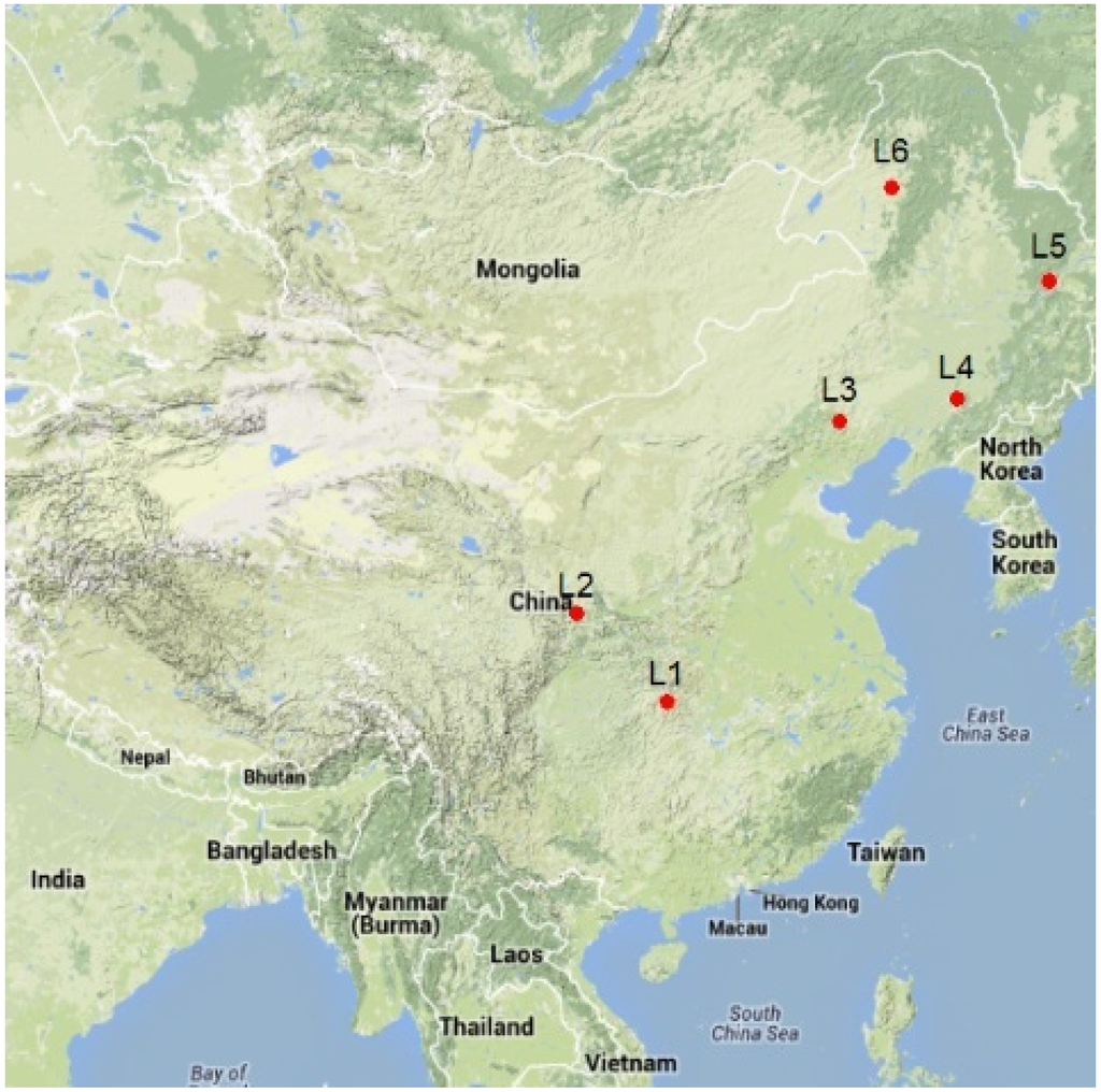
Figure 1. Six larch plantation regions in China.

Figure 1. Six larch plantation regions in China.

All subsamples were dried at 80°C and weighed to determine the dry biomass percentage for each part of the tree. The dry weight was calculated as the fresh weight of each part multiplied by the corresponding dry biomass percentage, while the total dry biomass for the tree was determined by summing the dry weights of different parts of the sampled tree (Table 2).

Table 2. Descriptive statistics of trees sampled for fitting the biomass equations (Std, standard deviation).

Regions	DBH(cm)		Stem Wood (Kg)		Stem Bark (Kg)		Branch (Kg)		Foliage (Kg)		Root (Kg)		Total (Kg)
	Mean	Std	Mean	Std	Mean	Std	Mean	Std	Mean	Std	Mean	Std	Mean	Std
L1	16.5	5.9	68.9	53.6	9.9	7.7	10.9	6.0	3.8	2.9	23.6	12.3	117.2	80.9
L2	13.0	6.6	38.7	45.9	5.7	5.8	7.0	6.7	2.3	2.2	13.2	16.3	77.0	80.2
L3	11.5	4.6	35.1	35.0	5.2	5.1	13.2	14.1	3.4	3.5	11.2	12.7	99.5	68.3
L4	14.5	5.5	78.4	81.9	8.5	7.2	8.4	6.8	3.5	2.7	18.4	19.6	155.1	115.8
L5	17.8	4.6	87.1	54.6	9.5	4.9	10.7	5.0	3.3	1.2	20.5	13.9	146.4	69.3
L6	12.4	6.0	55.6	60.9	6.5	6.3	6.3	6.7	1.6	1.6	20.3	21.0	73.0	74.5

Table 2. Descriptive statistics of trees sampled for fitting the biomass equations (Std, standard deviation).

Regions	DBH(cm)		Stem Wood (Kg)		Stem Bark (Kg)		Branch (Kg)		Foliage (Kg)		Root (Kg)		Total (Kg)
	Mean	Std	Mean	Std	Mean	Std	Mean	Std	Mean	Std	Mean	Std	Mean	Std
L1	16.5	5.9	68.9	53.6	9.9	7.7	10.9	6.0	3.8	2.9	23.6	12.3	117.2	80.9
L2	13.0	6.6	38.7	45.9	5.7	5.8	7.0	6.7	2.3	2.2	13.2	16.3	77.0	80.2
L3	11.5	4.6	35.1	35.0	5.2	5.1	13.2	14.1	3.4	3.5	11.2	12.7	99.5	68.3
L4	14.5	5.5	78.4	81.9	8.5	7.2	8.4	6.8	3.5	2.7	18.4	19.6	155.1	115.8
L5	17.8	4.6	87.1	54.6	9.5	4.9	10.7	5.0	3.3	1.2	20.5	13.9	146.4	69.3
L6	12.4	6.0	55.6	60.9	6.5	6.3	6.3	6.7	1.6	1.6	20.3	21.0	73.0	74.5

2.2. Bayesian Approach

By modelling the observed data and unobserved variables, regions can be regarded as random variables. The Bayesian approach provides a cohesive framework for combining hierarchical data models and external knowledge [22,26]. The Bayesian method is a statistical framework based on combining data with prior information about parameter values to derive probabilities of the various parameter values [27,28]. In our analysis, the distributional model f(y|θ) represents the biomass data y = (y₁,. . .,y_j) given a parameter vector θ = (θ₁, . . .,θ_j). Then, π(θ|λ) is determined, where λ is a hyperparameter vector [29]. The inference parameter θ is based on its posterior distribution:

$$p(\theta |y,\lambda )=\frac{p(y,\theta |\lambda )}{{\displaystyle \int p(y,\theta |\lambda )d\theta }}=\frac{f(y|\theta )\pi (\theta |\lambda )}{{\displaystyle \int f(y|\theta )\pi (\theta |\lambda )d\theta }}$$

(1)

This posterior distribution is used for a Bayesian statistical inference, in contrast to the Frequentist method, which uses f(y|θ) for inference. The f(y|θ) provides the distribution of y assuming θ is known, which is considered a likelihood function when viewed as a function of the parameters. The prior distributions of π(θ|λ) can be obtained from parameters reported in the literatureor using vague priors.

2.3. Allometric Models

Numerous models have been developed for estimating tree biomass, especially based on the allometric equations: W = aDBH^b and W = a(DBH²H)^b (where W is the tree biomass, DBH is the diameter at breast height, and H is the tree height). DBH is often used in biomass equations [11,30,31] and is more easily obtained than H. Therefore, W = aDBH^b was applied as the biomass model in this study. However, a heteroscedasticity exists when directly fitting tree biomass. Typically, logarithms (ln(W) = ln(a + b) ln(DBH)) can counteract heteroscedasticity [32]. Thus, the total tree, root, stem wood, stem bark, branch and foliage biomasses were modelled using the following log-transformed allometric equation:

$$y_i=a+b{x}_i+e_i$$

(2)

where y_i is the log-transformed biomass of each part of the ith sampled tree, x_i is the log-transformed DBH of the ith sampled tree, and a and b are the intercept and slope, respectively. The error term e_i assumes a normal distribution with a mean of zero and constant variance σ².

2.4. Modelling Approaches

2.4.1. Non-Hierarchical Bayesian Approach

The non-hierarchical Bayesian structure is shown in Figure 2. The observed values x_i are shown at the bottom. θ represents the unknown parameters of a and b associated with probability distribution f (y|θ). In the non-hierarchical Bayesian approach, the parameters in Equation (2) are treated as random variables. This approach was used to fit Equation (2), as given by:

$$p(a,b|data)={\displaystyle \prod _i\frac{1}{\sqrt{2\pi }{\sigma }^2}}\exp (\frac{-{(y_i-g(x_i:a,b))}^2}{2{\sigma }^2})$$

(3)

Figure 2. Bayesian non-hierarchical structure.

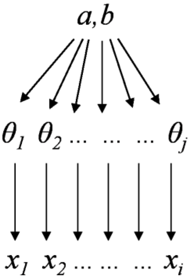
Figure 2. Bayesian non-hierarchical structure.

2.4.2. Hierarchical Bayesian Approach

Our data were collected fromsix different spatial regions and four species, which exhibit typical hierarchical data characteristics (Table 1). Figure 3 summarizes the hierarchical Bayesian approach. The biomass data can be used to estimate parameter θ_i for each region. Thus, the allometric equation for the hierarchical Bayesian approach can be written as follows:

$$y_{j(i)}=a_j+b_j{x}_{j(i)}+e_i$$

(4)

where y_j(i) and x_j(i) are the log-transformed biomass y and DBH of the ith tree in the jth region, respectively, and a_j and b_j are the intercept and slope of the jth region. The error term e_i assumes a normal distribution with a mean of zero and constant variance.

Our analysis hierarchically interprets the parameter estimation problem using cross-regional biomass data (Figure 3). Parameters a_j and b_j have specific values for each region, allowing for polymorphic lines and multiple asymptotes. For the jth region of theith tree, the parameter θ_j in Equation (4) is defined as:

$${\theta }_j=(a_j,b_j)=\left[\begin{array}{l}a+a_i\\ b+b_i\end{array}\right]$$

(5)

The hierarchical Bayesian approach is used to fit Equation (4), as given by:

$$p(a,b|data)=p(a,b){\displaystyle \prod _{j=1}^J\frac{\mathrm{\Gamma }(a+b)}{\mathrm{\Gamma }(a)\mathrm{\Gamma }(b)}}\frac{\mathrm{\Gamma }(a+y_j)\mathrm{\Gamma }(b+n_j-y_j)}{\mathrm{\Gamma }(a+b+n_j)}$$

(6)

where n_j is the number of regions.

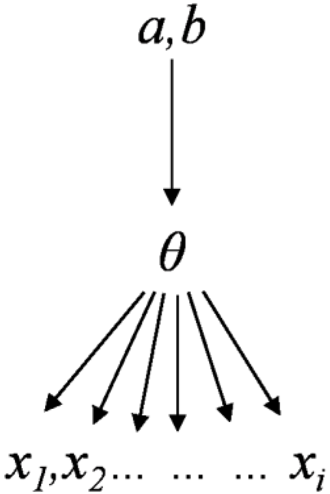
Figure 3. Bayesian hierarchical structure.

Figure 3. Bayesian hierarchical structure.

2.5. Prior Parameter Distributions

The choice of prior distributions for each parameter is critical in the Bayesian method [33]. Zhang et al. [10] found that Bayesian analyses with non-informative priors and a classic statistical approach yielded results that were similar to using parameters and statistics to fit allometric biomass equations. However, the Bayesian method with informative priors performed better than the non-informative priors and classic statistical approach. Thus, the appropriate prior distribution selections for all parameters are critical for improving the model precision. The prior distribution information can be obtained from parameters reported in the literature. In this study, the prior distributions of a and b (total tree, root, stem wood, stem bark, branch and foliage) were obtained for 36 biomass equations from 6 Chinese larch publications (Table S1). We assumed that a and b follow a bivariate normal distribution $N(\mu ,\mathrm{\Sigma })$, where $\mu ({\mu }_a,{\mu }_b)$ is a vector of means and $\mathrm{\Sigma }$ is the covariance matrix (Table 3).

Table 3. Prior parameter distributions from the published literature for each equation.

Component	${\mathbf{\mu }}_{\mathit{a}}$	${\mathbf{\mu }}_{\mathit{b}}$	$\mathbf{\Sigma }$
Total tree	−1.834	0.843	$\left(\begin{array}{ll}0.248& -0.032\\ -0.032& 0.006\end{array}\right)$
Root	−3.769	0.856	$\left(\begin{array}{ll}0.232& -0.302\\ -0.302& 0.060\end{array}\right)$
Stem wood	−2.649	0.888	$\left(\begin{array}{ll}0.214& -0.022\\ -0.022& 0.004\end{array}\right)$
Stem bark	−3.539	0.694	$\left(\begin{array}{ll}1.056& -0.149\\ -0.149& 0.031\end{array}\right)$
Branch	−3.113	0.641	$\left(\begin{array}{ll}2.370& -0.375\\ -0.375& 0.089\end{array}\right)$
Foliage	−3.719	0.597	$\left(\begin{array}{ll}2.608& -0.303\\ -0.303& 0.056\end{array}\right)$

Table 3. Prior parameter distributions from the published literature for each equation.

Component	${\mathbf{\mu }}_{\mathit{a}}$	${\mathbf{\mu }}_{\mathit{b}}$	$\mathbf{\Sigma }$
Total tree	−1.834	0.843	$\left(\begin{array}{ll}0.248& -0.032\\ -0.032& 0.006\end{array}\right)$
Root	−3.769	0.856	$\left(\begin{array}{ll}0.232& -0.302\\ -0.302& 0.060\end{array}\right)$
Stem wood	−2.649	0.888	$\left(\begin{array}{ll}0.214& -0.022\\ -0.022& 0.004\end{array}\right)$
Stem bark	−3.539	0.694	$\left(\begin{array}{ll}1.056& -0.149\\ -0.149& 0.031\end{array}\right)$
Branch	−3.113	0.641	$\left(\begin{array}{ll}2.370& -0.375\\ -0.375& 0.089\end{array}\right)$
Foliage	−3.719	0.597	$\left(\begin{array}{ll}2.608& -0.303\\ -0.303& 0.056\end{array}\right)$

2.6. Model Fitting

Using the non-hierarchical Bayesian approach as a base method, we used the nonlinear extra sum of squares method and the Lakkis-Jones test to assess whether the hierarchical Bayesian approach significantly improved the accuracy of the biomass equation [34,35]. The statistics are given by thenonlinear extra sum of squares:

$$F=(\frac{SS{E}_N-SS{E}_B}{d{f}_N-d{f}_B})\frac{d{f}_B}{SS{E}_B}$$

(7)

And Lakkis-Jones test:

$$L=2Ln({(\frac{SS{E}_N}{SS{E}_B})}^{\frac{n}{2}})$$

(8)

where $SS{E}_N$ is the sum of squares of residuals in the non-hierarchical Bayesian approach, $SS{E}_B$ is the sum of squares of residuals in the hierarchical Bayesian approach, $d{f}_N$ and $d{f}_B$ are the degrees of freedom of the non-hierarchical and hierarchical Bayesian approaches, respectively, and n is the number of observations used in the model fitting. The F-statistic follows an F-distribution, and the L-statistic follows a ${\chi }^2$-distribution with $v=d{f}_N-d{f}_B$ degrees of freedom.

The Markov Chain Monte Carlo (MCMC) algorithm was used to estimate model parameters in both non-hierarchical and hierarchical Bayesian approaches. All models were fitted using the MCMC method in the MCMCglmm package and R2WinBUGS package in R version 3.1.1 [36,37].

3. Results

3.1. Fitted Biomass Models

This study compiled 36 logarithmic biomass equations for larch biomass in China. The prior parameter distributions were obtained from the published literature. Parameters a and b followed bivariate normal distributions in each component biomass model (Table 3). Based on the Bayesian theory with informative priors, we obtained the posterior probability distributions of the two parameters for each component biomass model. The values of a and b for the total tree and component biomass models were estimated using non-hierarchical and hierarchical Bayesian approaches.

The posterior total tree biomassprobability distributions are shown in Figure 4, which are similar to the posterior probability distributions of the component biomass model. According to the fitted results, the total tree, root, stem wood, stem bark, branch and foliage (p-values < 0.001) biomass model relationships were significant for both the non-hierarchical and hierarchical Bayesian approaches. 10,000 iterations were performed for each model fitting to ensure convergence and obtain posterior distributions of the estimated parameters. Of these, the first 500 were discarded as burn-in iterations. The thinning parameter between the non-hierarchical and hierarchical approaches was set at three chains to reduce the impact of the correlation between neighbouring iterations. The standard deviation (S.D.) and P_2.5%–P_97.5% were then calculated based on the samples. The parameter estimates using the non-hierarchical and hierarchical Bayesian approaches are presented in Table 4 and Table 5.

Table 4. Tree biomass model parameters using the Bayesian non-hierarchical approach.

Component	Parameters	Mean	S.D.	P2.5%–P97.5%
Total tree	a	−2.117	0.054	(−2.225 −2.012)
	b	2.42	0.021	(2.379 2.462)
Root	a	−3.963	0.092	(−4.146 −3.784)
	b	2.459	0.036	(2.389 2.530)
Stem wood	a	−3.521	0.081	(−3.684 −3.362)
	b	2.728	0.032	(2.666 2.791)
Stem bark	a	−3.927	0.093	(−4.113 −3.746)
	b	2.152	0.036	(2.018 2.224)
Branch	a	−2.682	0.15	(−2.225 −2.012)
	b	1.783	0.059	(−2.225 −2.012)
Foliage	a	−3.28	0.176	(−3.631 −2.937)
	b	1.578	0.069	(1.444 1.715)

Table 4. Tree biomass model parameters using the Bayesian non-hierarchical approach.

Component	Parameters	Mean	S.D.	P2.5%–P97.5%
Total tree	a	−2.117	0.054	(−2.225 −2.012)
	b	2.42	0.021	(2.379 2.462)
Root	a	−3.963	0.092	(−4.146 −3.784)
	b	2.459	0.036	(2.389 2.530)
Stem wood	a	−3.521	0.081	(−3.684 −3.362)
	b	2.728	0.032	(2.666 2.791)
Stem bark	a	−3.927	0.093	(−4.113 −3.746)
	b	2.152	0.036	(2.018 2.224)
Branch	a	−2.682	0.15	(−2.225 −2.012)
	b	1.783	0.059	(−2.225 −2.012)
Foliage	a	−3.28	0.176	(−3.631 −2.937)
	b	1.578	0.069	(1.444 1.715)

Table 5. Tree biomass model parameters using the Bayesian hierarchical approach (a₁–a₆ and b₁–b₆ represent the six regions from L1–L6).

Parameters	Total Tree			Root
	Mean	S.D	P2.5%–P97.5%	Mean	S.D	P2.5%–P97.5%
a1	−1.878	0.159	(−2.173 −1.554)	−2.041	0.314	(−2.660 −1.417)
a2	−1.849	0.076	(−1.994 −1.700)	−3.929	0.133	(−4.191 −3.671)
a3	−2.298	0.095	(−2.485 −2.113)	−4.653	0.170	(−4.981 −4.318)
a4	−2.650	0.137	(−2.919 −2.381)	−4.412	0.222	(−4.842 −3.991)
a5	−1.451	0.134	(−1.712 −1.190)	−3.135	0.219	(−3.563 −2.704)
a6	−2.540	0.104	(−2.739 −2.330)	−4.030	0.186	(−4.399 −3.670)
b1	2.307	0.058	(2.188 2.413)	1.829	0.114	(1.604 2.053)
b2	2.277	0.032	(2.214 2.338)	2.434	0.056	(2.325 2.543)
b3	2.519	0.040	(2.442 2.598)	2.705	0.071	(2.563 2.843)
b4	2.649	0.052	(2.546 2.752)	2.600	0.084	(2.439 2.763)
b5	2.208	0.049	(2.113 2.304)	2.138	0.080	(1.980 2.295)
b6	2.554	0.041	(2.471 2.635)	2.551	0.074	(2.406 2.698)
Parameters	Stem Wood			Stem Bark
	Mean	S.D	P2.5%−P97.5%	Mean	S.D	P2.5%−P97.5%
a1	−4.394	0.250	(−4.894 −3.915)	−3.971	0.134	(−4.251 −3.741)
a2	−3.114	0.122	(−3.356 −2.880)	−3.927	0.102	(−4.119 −3.721)
a3	−3.356	0.152	(−3.649 −3.057)	−3.904	0.106	(−4.105 −3.684)
a4	−4.284	0.210	(−4.687 −3.863)	−3.916	0.118	(−4.151 −3.685)
a5	−3.007	0.195	(−3.402 −2.634)	−3.897	0.115	(−4.110 −3.657)
a6	−3.843	0.153	(−4.143 −3.542)	−3.965	0.111	(−4.185 −3.751)
b1	2.971	0.091	(2.796 3.153)	2.151	0.048	(2.067 2.247)
b2	2.525	0.051	(2.427 2.628)	2.146	0.042	(2.062 2.226)
b3	2.671	0.063	(2.546 2.794)	2.150	0.043	(2.062 2.231)
b4	3.061	0.080	(2.900 3.214)	2.166	0.046	(2.078 2.261)
b5	2.597	0.071	(2.462 2.742)	2.153	0.042	(2.067 2.232)
b6	2.836	0.061	(2.714 2.955)	2.142	0.043	(2.057 2.225)
Parameters	Branch			Foliage
	Mean	S.D	P2.5%–P97.5%	Mean	S.D	P2.5%–P97.5%
a1	−2.374	0.381	(−3.080 −1.599)	−2.867	0.477	(−3.796 −1.928)
a2	−2.757	0.192	(−3.130 −2.376)	−2.958	0.258	(−3.472 −2.466)
a3	−3.387	0.282	(−3.931 −2.818)	−4.702	0.337	(−5.358 −4.049)
a4	−2.354	0.322	(−2.958 −1.705)	−2.274	0.421	(−3.119 −1.471)
a5	−1.989	0.343	(−2.666 −1.331)	−1.659	0.422	(−2.473 −0.843)
a6	−3.277	0.255	(−3.783 −2.787)	−4.225	0.339	(−4.894 −3.558)
b1	1.673	0.138	(1.392 1.928)	1.434	0.173	(1.093 1.771)
b2	1.794	0.081	(1.633 1.948)	1.429	0.108	(1.221 1.649)
b3	2.287	0.118	(2.045 2.515)	2.268	0.141	(1.994 2.539)
b4	1.605	0.123	(1.359 1.835)	1.263	0.161	(0.952 1.538)
b5	1.543	0.125	(1.303 1.791)	1.020	0.154	(0.721 1.326)
b6	1.835	0.101	(1.640 2.036)	1.717	0.135	(1.454 1.983)

Table 5. Tree biomass model parameters using the Bayesian hierarchical approach (a₁–a₆ and b₁–b₆ represent the six regions from L1–L6).

Parameters	Total Tree			Root
	Mean	S.D	P2.5%–P97.5%	Mean	S.D	P2.5%–P97.5%
a1	−1.878	0.159	(−2.173 −1.554)	−2.041	0.314	(−2.660 −1.417)
a2	−1.849	0.076	(−1.994 −1.700)	−3.929	0.133	(−4.191 −3.671)
a3	−2.298	0.095	(−2.485 −2.113)	−4.653	0.170	(−4.981 −4.318)
a4	−2.650	0.137	(−2.919 −2.381)	−4.412	0.222	(−4.842 −3.991)
a5	−1.451	0.134	(−1.712 −1.190)	−3.135	0.219	(−3.563 −2.704)
a6	−2.540	0.104	(−2.739 −2.330)	−4.030	0.186	(−4.399 −3.670)
b1	2.307	0.058	(2.188 2.413)	1.829	0.114	(1.604 2.053)
b2	2.277	0.032	(2.214 2.338)	2.434	0.056	(2.325 2.543)
b3	2.519	0.040	(2.442 2.598)	2.705	0.071	(2.563 2.843)
b4	2.649	0.052	(2.546 2.752)	2.600	0.084	(2.439 2.763)
b5	2.208	0.049	(2.113 2.304)	2.138	0.080	(1.980 2.295)
b6	2.554	0.041	(2.471 2.635)	2.551	0.074	(2.406 2.698)
Parameters	Stem Wood			Stem Bark
	Mean	S.D	P2.5%−P97.5%	Mean	S.D	P2.5%−P97.5%
a1	−4.394	0.250	(−4.894 −3.915)	−3.971	0.134	(−4.251 −3.741)
a2	−3.114	0.122	(−3.356 −2.880)	−3.927	0.102	(−4.119 −3.721)
a3	−3.356	0.152	(−3.649 −3.057)	−3.904	0.106	(−4.105 −3.684)
a4	−4.284	0.210	(−4.687 −3.863)	−3.916	0.118	(−4.151 −3.685)
a5	−3.007	0.195	(−3.402 −2.634)	−3.897	0.115	(−4.110 −3.657)
a6	−3.843	0.153	(−4.143 −3.542)	−3.965	0.111	(−4.185 −3.751)
b1	2.971	0.091	(2.796 3.153)	2.151	0.048	(2.067 2.247)
b2	2.525	0.051	(2.427 2.628)	2.146	0.042	(2.062 2.226)
b3	2.671	0.063	(2.546 2.794)	2.150	0.043	(2.062 2.231)
b4	3.061	0.080	(2.900 3.214)	2.166	0.046	(2.078 2.261)
b5	2.597	0.071	(2.462 2.742)	2.153	0.042	(2.067 2.232)
b6	2.836	0.061	(2.714 2.955)	2.142	0.043	(2.057 2.225)
Parameters	Branch			Foliage
	Mean	S.D	P2.5%–P97.5%	Mean	S.D	P2.5%–P97.5%
a1	−2.374	0.381	(−3.080 −1.599)	−2.867	0.477	(−3.796 −1.928)
a2	−2.757	0.192	(−3.130 −2.376)	−2.958	0.258	(−3.472 −2.466)
a3	−3.387	0.282	(−3.931 −2.818)	−4.702	0.337	(−5.358 −4.049)
a4	−2.354	0.322	(−2.958 −1.705)	−2.274	0.421	(−3.119 −1.471)
a5	−1.989	0.343	(−2.666 −1.331)	−1.659	0.422	(−2.473 −0.843)
a6	−3.277	0.255	(−3.783 −2.787)	−4.225	0.339	(−4.894 −3.558)
b1	1.673	0.138	(1.392 1.928)	1.434	0.173	(1.093 1.771)
b2	1.794	0.081	(1.633 1.948)	1.429	0.108	(1.221 1.649)
b3	2.287	0.118	(2.045 2.515)	2.268	0.141	(1.994 2.539)
b4	1.605	0.123	(1.359 1.835)	1.263	0.161	(0.952 1.538)
b5	1.543	0.125	(1.303 1.791)	1.020	0.154	(0.721 1.326)
b6	1.835	0.101	(1.640 2.036)	1.717	0.135	(1.454 1.983)

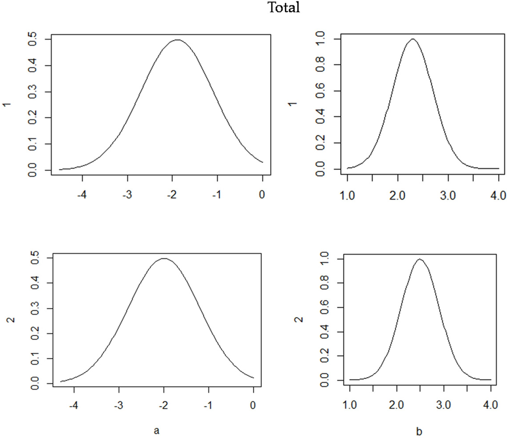
Figure 4. Posterior probability densities of two parameters for each total tree biomass model. 1 is the non-hierarchical approach, and 2 is the Bayesian hierarchical approach.

Figure 4. Posterior probability densities of two parameters for each total tree biomass model. 1 is the non-hierarchical approach, and 2 is the Bayesian hierarchical approach.

3.2. Comparison of Two BayesianApproaches

The p-values, R², nonlinear extra sum of squares (F-value) and the Lakkis-Jones (L-value) tests of the biomass model estimated by the non-hierarchical and hierarchical Bayesian approaches are shown in Table 6. We detected significant differences between the two Bayesian approaches with respect to the stem wood, foliage, branch, root and total tree biomass models (p-value < 0.001). The hierarchical Bayesian approach increased the goodness-of-fit statistics. The R² values of the total tree, root, stem wood, stem bark, branch and foliage biomass models using the hierarchical Bayesian method were 0.008, 0.018, 0.020, 0.003, 0.088 and 0.116 higher than non-hierarchical model, respectively.

Table 6. Evaluation of the non-hierarchical and hierarchical Bayesian approaches (1 and 2 represent the non-hierarchical and hierarchical Bayesian approaches, respectively).

Component	Approach	p-Values	R2	F-Values	Pr > |F|	L-Values	Pr > |L|
Total tree	1	<0.001	0.981
	2	<0.001	0.989	7.071	<0.001	154.386	<0.001
Root	1	<0.001	0.950
	2	<0.001	0.968	6.097	<0.001	137.493	<0.001
Stem wood	1	<0.001	0.967
	2	<0.001	0.987	5.561	<0.001	127.443	<0.001
Stem bark	1	<0.001	0.934
	2	<0.001	0.937	0.392	0.264	10.354	0.264
Branch	1	<0.001	0.791
	2	<0.001	0.879	7.575	<0.001	136.152	<0.001
Foliage	1	<0.001	0.682
	2	<0.001	0.798	6.039	<0.001	165.496	<0.001

Table 6. Evaluation of the non-hierarchical and hierarchical Bayesian approaches (1 and 2 represent the non-hierarchical and hierarchical Bayesian approaches, respectively).

Component	Approach	p-Values	R2	F-Values	Pr > |F|	L-Values	Pr > |L|
Total tree	1	<0.001	0.981
	2	<0.001	0.989	7.071	<0.001	154.386	<0.001
Root	1	<0.001	0.950
	2	<0.001	0.968	6.097	<0.001	137.493	<0.001
Stem wood	1	<0.001	0.967
	2	<0.001	0.987	5.561	<0.001	127.443	<0.001
Stem bark	1	<0.001	0.934
	2	<0.001	0.937	0.392	0.264	10.354	0.264
Branch	1	<0.001	0.791
	2	<0.001	0.879	7.575	<0.001	136.152	<0.001
Foliage	1	<0.001	0.682
	2	<0.001	0.798	6.039	<0.001	165.496	<0.001

The performance of all fitted models is shown in Figure 5. Boxplots illustrate the residual tendency of each biomass model component for the two Bayesian approaches in each region. The hierarchical Bayesian approach residuals are closer to both the zero-line and the observed values compared to those of the non-hierarchical Bayesian approach. Thus, the hierarchical approach yielded more accurate parameter estimates.

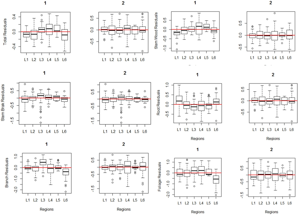
Figure 5. Residual boxplots comparing the non-hierarchical and hierarchical Bayesian approaches. 1 and 2 represent the non-hierarchical and hierarchical Bayesian approaches, respectively.

Figure 5. Residual boxplots comparing the non-hierarchical and hierarchical Bayesian approaches. 1 and 2 represent the non-hierarchical and hierarchical Bayesian approaches, respectively.

4. Discussion

Theoretical Bayesian methods have been gradually adapted to plant biomass estimations [9,10,15,16]. Frequentist statistics assume that parameters are fixed, unknown constant values, whereas Bayesian statistics assume that parameters follow a statistical distribution. For example, Mauricio et al. [9] demonstrated that parameters were well represented by a bivariate normal distribution in an allometric biomass model. One advantage of the Bayesian approach is the MCMC algorithm [18,28,38], which avoids many of the approximations used by the frequentist method [39,40], improving the parameter estimation and model fit.

We establishedtotal tree and biomass component models using non-hierarchical and hierarchical Bayesian approaches. We found that the hierarchical approach performed better, and the hierarchical Bayesian approach significantly improved the accuracy of the biomass model, except for the stem bark model. The stem bark biomass may have accounted for a sufficiently small proportion of the total tree biomass. In general, the hierarchicalapproachperformed better and incorporated the effects of sampling location variability, tree density and other variable factors related to the model-fitting process.

Developing biomass models at large regional scales and improving model accuracy is a significant issue in forest biomass research. Mixed effects models and dummy variable methods are often used to improve the goodness of fit of biomass models [41,42]. When regional effects are present, hierarchical Bayesian approach can be applied to fit the biomass model. Because the data were collected from various spatial regions, biomass model parameters may regionally vary. These variations indicate that regional effects play important roles in the model-fitting process and may be related to unique regional characteristics, such as climate factors, standdensity, tree species or other less noticeable characteristics. The hierarchical approach may yield more realistic results when data are collected at large and spatially variable regional scales. By estimating the total tree and biomass component model variables with this approach, and combined with forest survey data, we can estimate the total and component biomass of stands from each region.

Our results indicate that the hierarchical Bayesian approach improved the model-fitting results, but additional studies may be required to further investigate the effectiveness of the hierarchical Bayesian approach for other species and in other regions. Future studies may also be required to confirm that this method is significantly better than the non-hierarchical approach. Note that, if the model fitting process accounts for species differences as a nested factor based on regional differences, the model fitting results should improve, and the hierarchical Bayesian approach would be more effective than the non-hierarchical method.

5. Conclusions

The larch biomass data were collected from different regions, including Hubei, Gansu, Hebei, Liaoning, Heilongjiang and Inner Mongolia, which encompass large climate, larch species, silviculture and stand density variations that affect biomass accumulation. These different biotic and abiotic factors introduce variabilities to the larch biomass model, suggesting that allometric equation parameters are better represented by probability distributions rather than fixed values. Therefore, a hierarchical Bayesian approach with informative priors is more suitable for fitting biomass models with regional variations. In this paper, we applied non-hierarchical and hierarchical Bayesian approaches to establish tree biomass models for larch plantations in six Chinese regions. Based on the fitting results, the total tree, root, stem wood, stem bark, branch and foliage biomass model relationships were significant (p-values < 0.001) for both the non-hierarchical and hierarchical Bayesian approaches.The hierarchical Bayesian approach increased the goodness-of-fit statistics compared to the non-hierarchical approach, significantly improving the accuracy of the biomass model (except for the stem bark) and providing an effective method for estimating larch biomass at the regional scale.

References

- China Forestry Bureau. The Eighth Forest Resource Survey Report; Chinese Forestry Press: Beijing, China, 2014; p. 18.
- Ares, A.; Fownes, J.H. Comparisons between generalized and specific tree biomass functions as applies to tropical ash (Fraxinusuhdei). New For. 2000, 20, 277–286. [Google Scholar] [CrossRef]
- Sah, J.P.; Ross, M.S.; Koptur, S.; Snyder, J.R. Estimating aboveground biomass of broadleaved woody plants in the understory of Florida Keys pine forests. For. Ecol. Manag. 2004, 203, 319–329. [Google Scholar] [CrossRef]
- Usuga, J.C.; Toro, J.A.R.; Alzate, M.V.R.; Tapias, A.J. Estimation of biomass and carbon stock in plants, soil and forest floor in different tropical forests. For. Ecol. Manag. 2010, 260, 1906–1913. [Google Scholar] [CrossRef]
- Jenkins, J.C.; Chojnacky, D.C.; Heath, L.S.; Birdsey, R.A. National-scale biomass estimators for United States tree species. For. Sci. 2003, 49, 12–35. [Google Scholar]
- Zianis, D.; Muukkonen, P.; Makipaa, R.; Mencuccini, M. Biomass and stem volume equations for tree species in Europe. Silva Fenn. Monogr. 2005, 4, 1–63. [Google Scholar]
- Navar, J. Biomass component equations for Latin American species and groups of species. Ann. For. Sci. 2009, 66, 208. [Google Scholar] [CrossRef]
- Nafus, A.M.; McClaran, M.P.; Archer, S.R.; Throop, H.L. Multispecies allometric models predict grass biomass in semidesert rangeland. Rangel. Ecol. Manag. 2009, 62, 68–72. [Google Scholar] [CrossRef]
- Mauricio, Z.C.; Carlos, A.S.; Lauren, A. Probability distribution of allometric coefficients and Bayesian estimation of aboveground tree biomass. For. Ecol. Manag. 2012, 277, 173–179. [Google Scholar]
- Zhang, X.Q.; Duan, A.G.; Zhang, J.G. Tree biomass estimation of Chinese fir (Cunninghamialanceolata) based on Bayesian method. PLoS ONE 2013, 8, e79868. [Google Scholar] [CrossRef] [PubMed]
- Zianis, D.; Mencuccini, M. On simplifying allometric analyses of forest biomass. For. Ecol. Manag. 2004, 187, 311–332. [Google Scholar] [CrossRef]
- Zianis, D. Predicting mean aboveground forest biomass and its associated variance. For. Ecol. Manag. 2008, 256, 1400–1407. [Google Scholar] [CrossRef]
- Chesson, P. Mechanisms of maintenance of species diversity. Annu. Rev. Ecol. Syst. 2000, 31, 343–366. [Google Scholar] [CrossRef]
- Melbourne, B.A.; Hastings, A. Extinction risk depends strongly on factors contributing to stochasticity. Nature 2008, 454, 100–103. [Google Scholar] [CrossRef] [PubMed]
- Fox, G.A.; Kendall, B.E. Demographic stochasticity and the variance reduction effect. Ecology 2002, 83, 1928–1934. [Google Scholar] [CrossRef]
- Pfister, C.A.; Stevens, F.R. Individual variation and environmental stochasticity: Implications for matrix model predictions. Ecology 2003, 84, 496–510. [Google Scholar] [CrossRef]
- Gilks, W.R.; Thomas, A.; Spiegelhalter, D.J. A language and program for complex Bayesian modelling. Statistician 1994, 43, 169–178. [Google Scholar] [CrossRef]
- Cowles, M.K.; Carlin, B.P. Markov chain Monte Carlo convergence diagnostics: A comparative review. J. Am. Stat. Assoc. 1996, 91, 883–904. [Google Scholar] [CrossRef]
- Myers, R.A.; Mertz, G. Reducing uncertainty in the biological basis of fisheries management by meta-analysis of data from many populations: A synthesis. Fish. Res. 1998, 37, 51–61. [Google Scholar] [CrossRef]
- Harley, S.J.; Myers, R.A.; Barrowman, N.J.; Bowen, K.G.; Amiro, R.E. Estimation of research trawl survey catchability for biomass reconstruction of the eastern Scotian Shelf. Res. Doc. 2001, 84, 1–53. [Google Scholar]
- Shelton, J.H.; Ransom, A. Hierarchical Bayesian models of length-specific catchability of research trawl surveys. Can. J. Fish. Aquat. Sci. 2001, 58, 1569–1584. [Google Scholar]
- Spiegelhalter, D.J.; Best, N.G.; Carlin, B.P.; Linde, A.V.G. Bayesian measures of model complexity and fit. J. R. Stat. Soc. 2002, 64, 583–640. [Google Scholar] [CrossRef]
- Green, E.J.; Strawderman, W.E. A comparison of hierarchical Bayes and empirical Bayes methods with a forestry application. For Sci. 1992, 38, 350–366. [Google Scholar]
- Finley, A.O.; Kittredge, D.B. Thoreau, Muir and Jane Doe: Different types of private forest owners need different kinds of forest management. North. J. Appl. For. 2006, 23, 27–34. [Google Scholar]
- Zhang, X.Q.; Zhang, J.G.; Duan, A.G. A hierarchical bayesian model to predict self-thinning line for Chinese fir(Cunninghamialanceolata) in southern China. PLoS ONE 2015, 10, e0139788. [Google Scholar] [CrossRef] [PubMed]
- Gelman, A.; Hill, J. Data Analysis Using Regression and Multilevel/Hierarchical Models; Cambridge University Press: Cambridge, UK, 2006; p. 58. [Google Scholar]
- Gelman, A. Analysis of variance: Why it is more important than ever. Ann. Stat. 2005, 33, 1–53. [Google Scholar] [CrossRef]
- Baayen, R.H.; Davidson, D.J.; Bates, D.M. Mixed-effects modeling with crossed random effects for subjects and items. J. Mem. Lang. 2008, 59, 390–412. [Google Scholar] [CrossRef]
- Carlin, B.P.; Louis, T.A. Bayes and Empirical Bayes Methods for Data Analysis; Monographs on Statistics and Applied Probability; Chapman & Hall: London, UK, 1996; Volume 69, p. 56. [Google Scholar]
- Heien, D.M. A note on log-linear regression. J. Am. Stat. Assoc. 1968, 63, 1034–1038. [Google Scholar]
- Ter-Mikaelian, M.T.; Korzukhin, M.D. Biomass equations for sixty-five North American tree species. For. Ecol. Manag. 1997, 97, 1–24. [Google Scholar] [CrossRef]
- Overman, J.P.M.; Witte, H.J.L.; Saldarriaga, J.G. Evaluation of regression models for above-ground biomass determination in Amazon rainforest. J. Trop. Ecol. 1994, 10, 207–218. [Google Scholar] [CrossRef]
- Wagner, H.; Tüchler, R. Bayesian estimation of random effects models for multivariate responses of mixed data. Comput. Stat. Data Anal. 2010, 54, 1206–1218. [Google Scholar] [CrossRef]
- Bates, D.M.; Watts, D.G. Nonlinear Regression Analysis and Its Applications; John Wiley & Sons: New York, NY, USA, 1988; p. 102. [Google Scholar]
- Barrio-Anta, M.; Balboa-Murias, M.; Castedo-Dorado, F.; Diéguez-Aranda, U.; Alvarez-González, J.G. An ecoregional model for estimating volume, biomass and carbon pools in maritime pine (Pinuspinaster Ait) stands in Galicia (northwestern Spain). For. Ecol. Manag. 2006, 223, 24–34. [Google Scholar] [CrossRef]
- Hadfield, J.D. MCMC methods for multi-response generalized linear mixed models: The MCMCglmm R package. J. Stat. Softw. 2010, 33, 1–22. [Google Scholar] [CrossRef]
- Sturtz, S.; Ligges, U.; Gelman, A. R2WinBUGS: A package for running WinBUGS from R. J. Stat. Softw. 2005, 12, 1–16. [Google Scholar] [CrossRef]
- Carlin, B.P.; Clark, J.S.; Gelfand, A.E. Hierarchical Modelling for the Environmental Sciences: Statistical Methods and Applications; Oxford University Press: Oxford, UK, 2006; p. 103. [Google Scholar]
- Paap, R. What are the advantages of MCMC based inference in latent variable models. Stat. Neerl. 2002, 56, 2–22. [Google Scholar] [CrossRef]
- MarcKéry. Introduction to WinBUGS for Ecologists: A Bayesian Approach to Regression, ANOVA, Mixed Models and Related Analyses; Library of Congress Cataloging: Washington, D.C., USA, 2010; p. 8. [Google Scholar]
- Cole, T.G.; Ewel, J.J. Allometric equations for four valuable tropical tree species. For. Ecol. Manag. 2006, 229, 351–360. [Google Scholar] [CrossRef]
- Pérez-Cruzado, C.; Rodríguez-Soalleiro, R. Improvement in accuracy of aboveground biomass estimation in Eucalyptus nitens plantations: Effect of bole sampling intensity and explanatory variables. For. Ecol. Manag. 2011, 261, 2016–2028. [Google Scholar] [CrossRef]
© 2016 by the authors; licensee MDPI, Basel, Switzerland. This article is an open access article distributed under the terms and conditions of the Creative Commons by Attribution (CC-BY) license (http://creativecommons.org/licenses/by/4.0/).