Spatial Variation of Biomass Carbon Density in a Subtropical Region of Southeastern China

Abstract

Spatial pattern information of forest biomass carbon (FBC) density in forest ecosystems plays an important role in evaluating carbon sequestration potentials and forest management. The spatial variation of FBC density in a subtropical region of southeastern China was studied using geostatistics combined with Moran’s I and geographical information systems (GIS). Forest biomass carbon density values were variable, ranging from 0.12 Mg ha⁻¹ to 182.12 Mg ha⁻¹, with an average of 27.33 Mg ha⁻¹. The FBC density had the strongest positive correlation with forest age, followed by forest litter and elevation. The FBC density had significant positive spatial autocorrelation revealed by global Moran’s I. Clear spatial patterns were observed based on local Moran’s I. High FBC density values were mainly distributed in the northwestern and southwestern parts of Zhejiang province, which were related to adopting long-term policy of forest conservation in these areas, while low FBC density values located in the middle part and southeastern coastal area of the study area due to low forest coverage and intensive management of economic forests. The Moran’s I combined with geostatistical interpolation proved to be a useful tool for studying spatial variation of FBC density.

1. Introduction

Global warming caused by increasing greenhouses such as carbon dioxide (CO₂) is now becoming a persistent concern in China and worldwide. Carbon sequestration is considered an important approach to mitigating the CO₂ concentration in the atmosphere [1]. Compared to other methods, such as engineering technology [2], forests are cost-effective carbon sinks for sequestering CO₂ [3]. Forest ecosystems store 289–363 Pg C in biomass [4,5,6], accounting for 77% of the global aboveground vegetation carbon [4]. Due to their enormous carbon pool and high productivity ability, forest ecosystems play an important part in the global C cycle [7].

The Kyoto Protocol report under the United Nations Framework Convention on Climate Change (UNFCCC) requires the industrialized countries to reduce their greenhouse gas emissions and suggests these countries increase afforestation to increase carbon (C) sequestration and thus to partially offset their CO₂ emission [8]. The report also requires that parties estimate the carbon stock in biomass, litter and soil, separately [9]. Therefore, the knowledge of size and distribution of forest biomass C stocks is of scientific and political importance [10].

Globally, a lot of work has been carried out to study the carbon storage in forest ecosystem [11,12,13]. However, most of these studies were focused on tropical, temperate and boreal forests. Few were related to carbon storage in the subtropical forests. In China, the biomass carbon storage at the national scale was studied using continuous forest inventory data [14,15,16]. However, the biomass carbon storage values estimated by different researchers have significant differences due to lack of information of spatial variation of biomass carbon density. Therefore, characterizing the size and spatial distribution of biomass carbon density at regional scale is important to estimate the current carbon storage of China and to contribute to further carbon sequestration studies and the promotion of better management of the forests [17,18].

To acquire accurate estimates of forest biomass carbon, reliable datasets providing information on forest types of sites within the entire region are required, as forest biomass carbon (FBC) density varies from place to place, controlled by a series of environmental factors at different spatial scales [19,20]. Over the last 35 year, geostatistical methods have been successfully used to investigate the spatial variability of environmental variables and to incorporate this information into mapping [21]. Compared to the other methods, geostatistics provides an effective way to facilitate quantification of the spatial variation and spatial interpolation [22]. Therefore, it is widely applied to analyze spatial heterogeneity of forest and soil distributions [21,22,23].

The main objectives of this study were (a) to characterize the spatial variability of FBC density in subtropical forest in eastern China; (b) to analyze the spatial patterns of FBC density and the corresponding site characteristics; and (c) to update regional FBC information with intensive sampling and to apply spatial analysis methods to produce an integrated distribution map.

2. Experimental Section

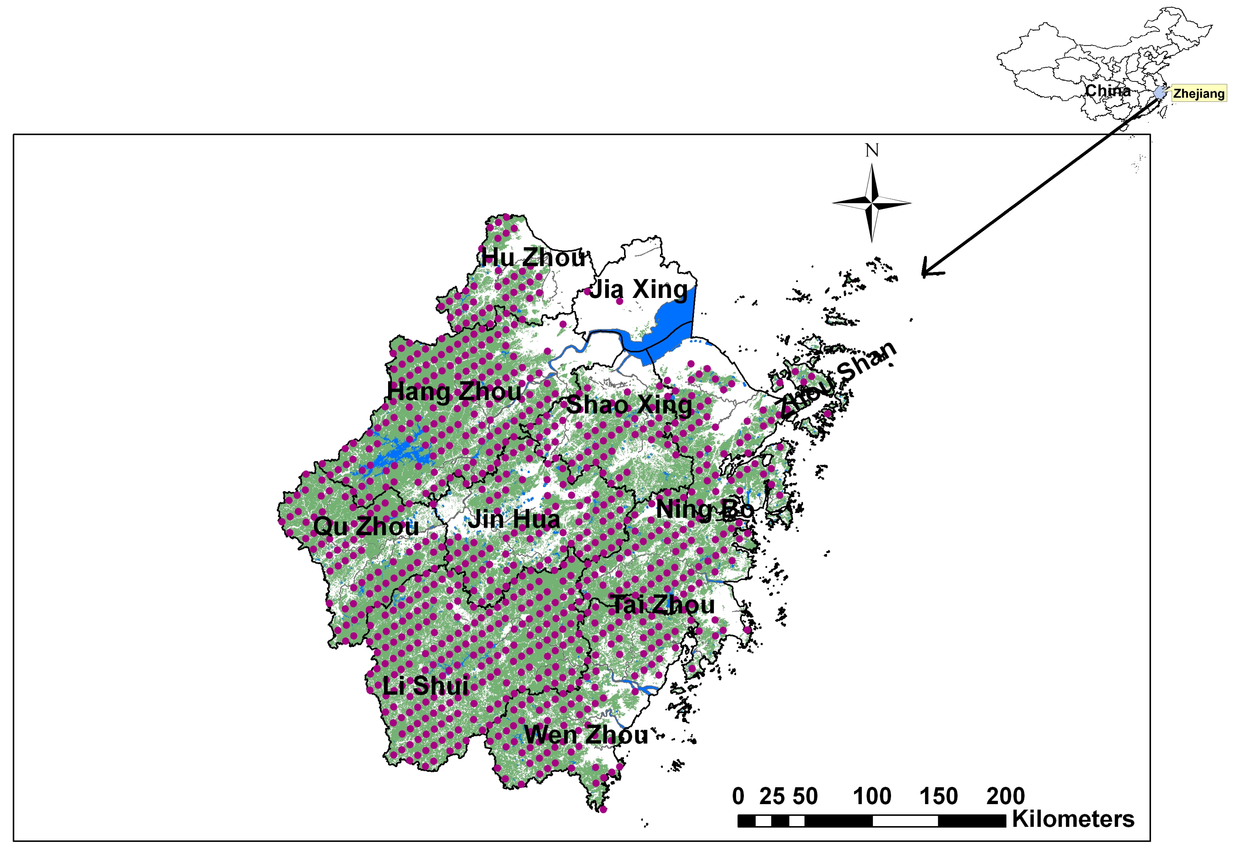
2.1. Study Area and Sampling Site Description

The study was carried out in Zhejiang province, southeastern China (Figure 1). Zhejiang province covers an area of 101,800 km² (118°01′ to 123°08′ E, 27°01′ to 31°10′ N). It has a typically subtropical marine monsoon climate with an average annual rainfall of 1490 mm and mean annual temperature of 16.5 °C. The main soil type is red soil [24]. From southwest to northeast, the elevation gradually decreases from 1603 m to 10 m. The province can be divided into four major agro-ecological regions: (1) Hang-Jia-Hu plain dominated by paddy fields; (2) Coastal region with quaternary marine deposition which has low agricultural production; (3) Inner hilly-basin region mainly of paddy fields and unirrigated croplands; and (4) Southwestern region of hills and uplands dominated by complexes of forest and dry croplands (ZJSS 1995). The total area of forest is approximate 58,442 km², accounting for 57.4% of total land area in Zhejiang Province [25]. The main forest types include evergreen broad-leaved forest, bamboo and other types (such as economic forest) [26]. The forest region in Zhejiang belongs to the Southern Collective Forest Region of China characterized by complex spatial distribution pattern, mixed agriculture and forestlands, various tree species, and intensive management.

Figure 1. Location of the study area and samples.

Figure 1. Location of the study area and samples.

In 2012, a total of 839 fixed forest plots were selected based on a 6 km (south-north) × 4 km (east-west) grid system (Figure 1). The longitudes and latitudes of the sampling points were recorded using a portable global positioning system (GPS) receiver. Relevant information related to the fixed forest plots including forest type, forest age, canopy density, elevation, slope aspect and position, individual tree biomass (aboveground and belowground biomass) and soil properties such as soil available N, P and K, soil pH was investigated and recorded. For each fixed forest plot, the total biomass was a sum of biomass of each tree in the plot. The individual tree biomass was calculated using biomass carbon model developed by Yuan et al. [26], which was based on long-term practical measurements and calculation in forest of Zhejiang province.

2.2. Data Analysis

The representative percentiles and commonly used descriptive statistics were calculated. Spearman correlation was conducted to study the correlation between FBC density and environmental variables. The differences of FBC density between different forest types were analyzed using analysis of variance (ANOVA). All the statistical analysis was carried out with SPSS 18.0 for Windows.

In the linear geostatistics method, a normal distribution for the studied variable is desired [27]. In this study, the data distributions were checked for normality with the Kolmogorov-Smirnov (K-S) test, and the forest biomass carbon density data was not normally distributed. Therefore, Box-Cox transformation performed by SAS software (version 9.1) was used for the following spatial autocorrelation analysis (Moran’s I) and spatial distribution analysis (geostatistics).

Moran’s I is a popularly used indicator of spatial autocorrelation and was applied to the calculated plot biomass carbon density data. In this study, global Moran’s I [28] was chosen as the first measure of spatial autocorrelation. Its values range from −1 to 1. The value “1” means strongly positive spatial autocorrelation, and “−1” indicates strongly negative spatial autocorrelation, and “0” implies spatial randomness [29].

While global Moran’s I suggests the presence or lack of spatial autocorrelation as a whole, the Local Indicators of Spatial Association (LISA) measures the degree of spatial autocorrelation in each specific location [30]. The Local Moran’s I is one of the LISA, representing the significant spatial clustering of similar values around a specific observation [25]. Local Moran’s I index can be expressed as:

$$I_i=\frac{Z_i-\stackrel{—}{Z}}{{\sigma }^{\mathrm{2}}}\sum _{j=\mathrm{1},j\ne \mathrm{1}}^n\left[W_{\mathit{ij}}\right(Z_j-\stackrel{—}{Z}\left)\right]$$

where $\overline{z}$ is the mean value of z with the sample number of n; z_i is the value at location i of the variable of interest; z_j is the value at other locations (where j ≠ i); σ² is the variance of z; and W_ij is a distance weighting between z_i and z_j, which can be defined as the inverse of the distance. The weight W_ij can also be determined using a distance band: samples situated at a distance smaller than the specified threshold distance considered as neighbors and given the same weight, while those outside the distance band are given the weight of 0. In this study, the free software Geoda [31] was used for the local Moran’s I calculation, and the distance band method to determine the W_ij was chosen.

Using Local Moran’s I can differentiate two types of spatial clusters (the target value is similar to its neighborhood): high-high clusters (location with high concentration in a neighborhood with high values), and low-low clusters (low values in a low value neighborhood), and two types of spatial outliers (the target value is obviously different from the values of its surrounding locations); and high-low (a high value in a low value neighborhood) and low-high (a low value in a high value neighborhood) [32].

The results of local Moran’s I can be standardized, so its significance level (P < 0.05 or 0.01) can be tested based on an assumption of a normal distribution [33]. This indicates that the clusters and the spatial outliers were significant at the 5% or 1% probability level. When using local Moran’s I index to analyze the spatial pattern, the results were affected by the definition of weight function, data transformation, and existence of extreme values. These factors were taken into consideration in order to obtain reliable and stable results. For the definition of weight function, the best distance band was obtained based on the largest global Moran’s I value, indicating the strongest spatial autocorrelation of FBC density. In this study, this distance band was 82.3 km, which was further used to study spatial clusters of biomass carbon density. Given the non-normality of the data, the Box-Cox transformed data was used. The transformed data can also eliminate the effect of extreme values on the spatial clusters analysis.

Our chosen method of geostatistical interpolation uses variogram (or semivariogram) to measure the spatial variability of a regionalized variable, and provides the input parameters for the spatial interpolation of kriging. Detailed information of this and related methods is widely available in textbooks [27,34]. In this study, ordinary kriging was applied to produce the spatial distribution maps. For the spatial interpolation, a cell size of 1 km × 1 km was chosen to divide the study area into a grid system of 712 columns (E-W direction) and 843 rows (N-S direction). The number of observations used for calculation was set to 12, as no clear improvement was found when more values were used. The chosen cell size was regarded as being effective to show the spatial patterns of the variable. The Box-Cox transformed data was used for interpolation and the corresponding kriging method is called trans-Gaussian kriging. We carried out the geostatistical interpolation with GS+ for win 7.0. All maps were produced using GIS software ArcMap^® (version 9.2).

3. Results and Discussion

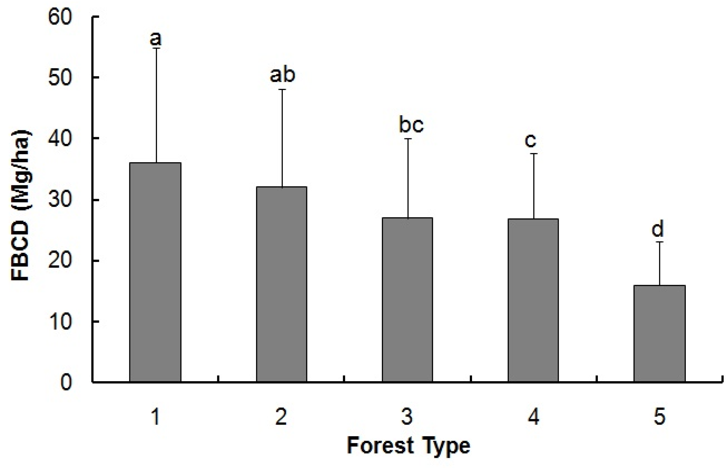
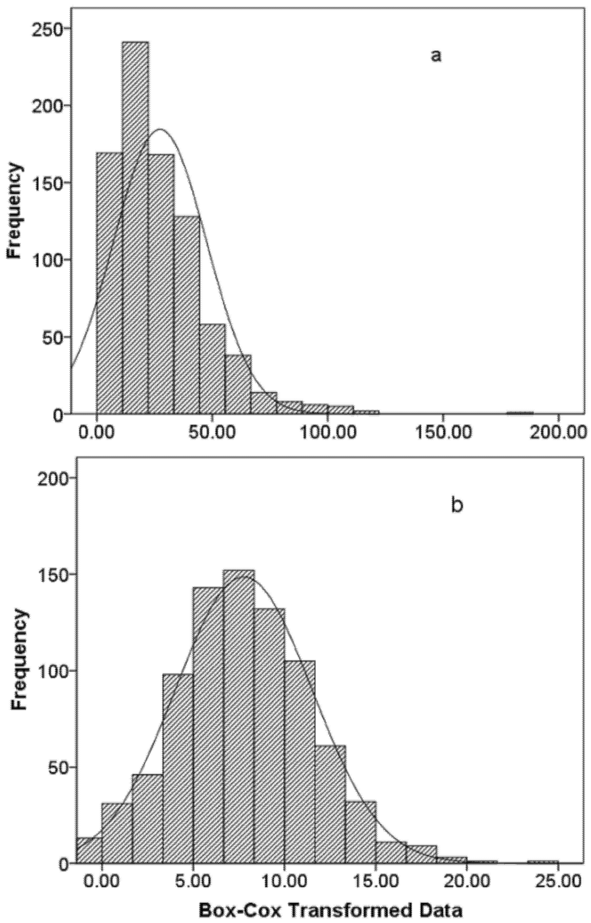
3.1. Descriptive Statistics of Forest Biomass Carbon Density

Forest biomass carbon density values were very variable (Table 1), ranging from 0.12 Mg ha⁻¹ to 182.12 Mg ha⁻¹, with an average of 27.33 Mg ha⁻¹. This average value was much lower than its counterparts in other Provinces of China, such as Sichuan (38.04 Mg ha⁻¹) [35], Fujian (32.85 Mg ha⁻¹) [36], Hainan (32.59 Mg ha⁻¹) [37], and Heilongjiang (45.68 Mg ha⁻¹) [38]. This was related to the young forest age in Zhejiang Province, as most of forest trees were planted in the last three decades [39]. The maximum and 95% percentile of the FBC density data were much larger than its upper quartile (75%), indicating positive skewed distribution of FBC density data, which was confirmed by the strongly positive skewness (1.72) and kurtosis (5.91) values. Compared to other parameters, the coefficient of variation (C.V.) value is the most discriminating factor for describing variability. When C.V. is less than 10%, it shows small variability; while when C.V. is more than 90%, it shows extensive variability [40]. In this study, the C.V. value of FBC density was 73.69%, indicating moderate variability in Zhejiang province.

Histograms of FBC density with a normal distribution curve are shown in Figure 2. The raw data have a long tail towards higher FBC density values (Figure 2a). Chang et al. [41], reported that environmental variables are often skewed from a normal distribution towards positive values because of the relatively smaller percentage of high values. The Box-Cox transformed data show a normal distribution (Figure 2b). This is confirmed by the K-S p value (>0.05, Table 1). Therefore, transformed data was used for geostatistical analysis.

Table 1. Descriptive statistics of forest biomass carbon density (Mg ha⁻¹, n = 839).

Min	5%	25%	Median	75%	95%	Max	Mean	SD	CV (%)	Skew	Kurt	K-Sp
0.12	1.45	13.48	22.81	37.16	142.61	182.12	27.33	20.14	73.69	1.72 (0.02)	5.91 (0.68)	0.00 (0.284)

Note: SD, standard deviation; CV, coefficient of variation; Skew, skewness, Kurt, kurtosis; K-S_p, significance level of Kolmogo-rov–Smirnov test for normality; Skew, Kurt and K-S_p values in brackets were calculated after Box-Cox transformation.

Table 1. Descriptive statistics of forest biomass carbon density (Mg ha⁻¹, n = 839).

Min	5%	25%	Median	75%	95%	Max	Mean	SD	CV (%)	Skew	Kurt	K-Sp
0.12	1.45	13.48	22.81	37.16	142.61	182.12	27.33	20.14	73.69	1.72 (0.02)	5.91 (0.68)	0.00 (0.284)

Note: SD, standard deviation; CV, coefficient of variation; Skew, skewness, Kurt, kurtosis; K-S_p, significance level of Kolmogo-rov–Smirnov test for normality; Skew, Kurt and K-S_p values in brackets were calculated after Box-Cox transformation.

Figure 2. Histograms of forest biomass carbon (FBC) density: (a) raw data; (b) Box-Cox transformed data with normal distribution curves.

Figure 2. Histograms of forest biomass carbon (FBC) density: (a) raw data; (b) Box-Cox transformed data with normal distribution curves.

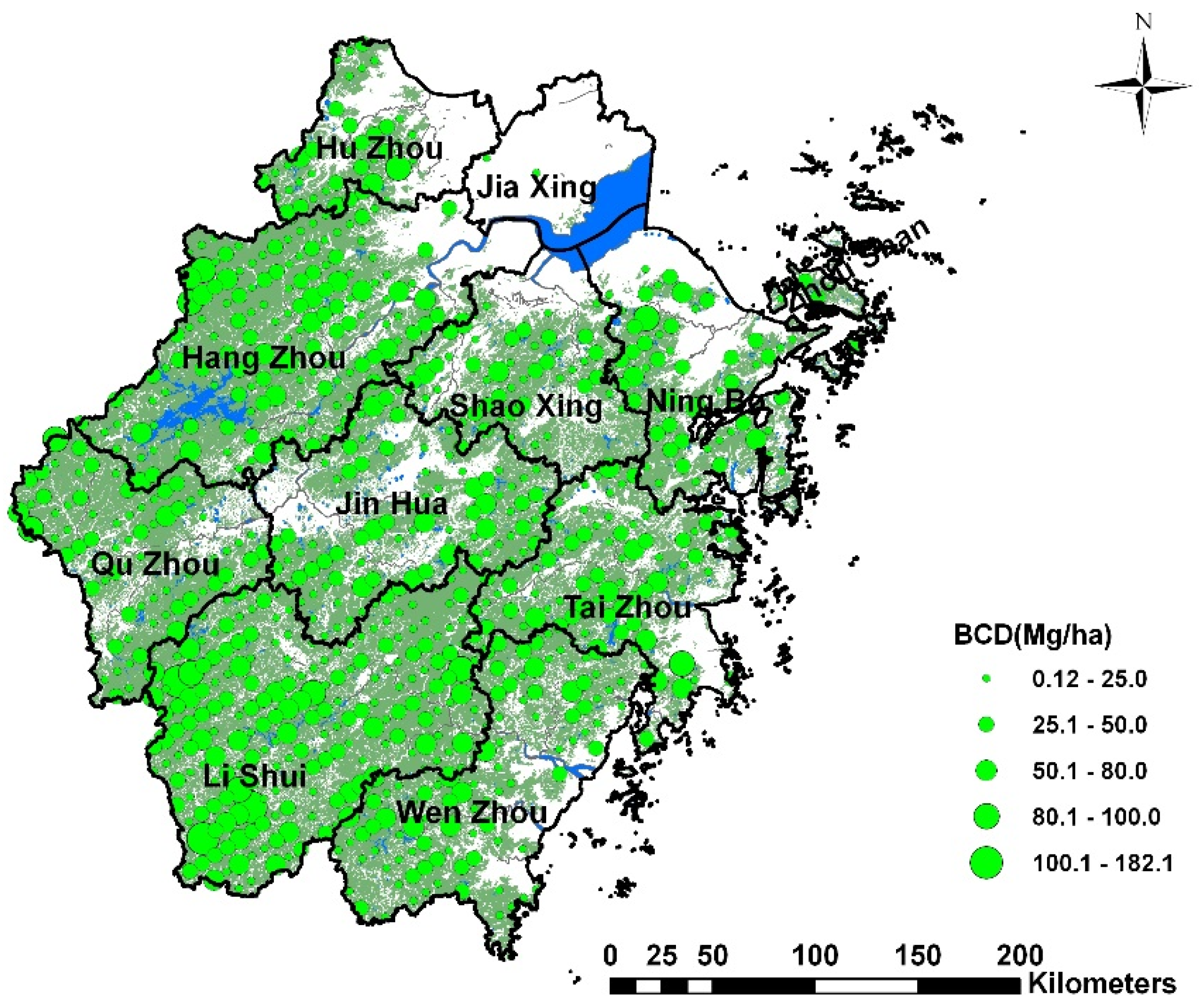
3.2. Spatial Symbol Map of Forest Biomass Carbon Density

A point symbol map of FBC density is shown in Figure 3. The majority of FBC density values ranged from 25.0 to 100.0 Mg ha⁻¹. Some high FBC density values were observed on the northwestern and southwestern parts of the study area, which were probably related to the long-term policy of forest conservation carried out by local governments in these areas. Low values were located in the middle part of Zhejiang province. This is mainly related to the intensive management by human beings, as the main forest type is economic forests, such as Chinese chestnut (Castanea mollissima) and Hickory (Carya cathayensis Sarg) forests. There were a number of scatted high FBC density values surrounded by relatively low values or low FBC density values surrounded by high values on the map, indicating the presence of spatial outliers.

Figure 3. Symbol map of forest biomass carbon (FBC) density values in Zhejiang province.

Figure 3. Symbol map of forest biomass carbon (FBC) density values in Zhejiang province.

3.3. The Environmental Factors Related to Forest Biomass Carbon Density

Spearman correlation coefficients between FBC density and environmental factors were calculated (Table 2). Positive and significant correlations between FBC density and elevation, forest age, forest litter carbon, soil organic carbon, and soil available nitrogen (N) were observed; while negative and significant correlations between FBC density and slope position and soil pH were found.

Table 2. Spearman correlation coefficients (n = 839).

	Elevation	Slope aspect	Slope position	Forest age	Forest litter carbon	Soil Organic carbon	Soil Available N	Soil pH	Soil Available P	Soil Available K
FBC	0.237 **	0.003	−0.166 **	0.468 **	0.306 **	0.176 **	0.124 **	−0.076 *	0.050	0.030
Elevation		−0.351 **	−0.016	0.071	0.188 **	0.208 **	0.268 **	0.016	0.030	0.243 **
Slope aspect			0.009	−0.034	−0.073 *	−0.037	−0.024	0.025	0.014	−0.021
Slope position				−0.136 **	−0.158 **	−0.083 *	−0.082 *	0.152 **	0.013	−0.041
Forest age					0.219 **	0.137 **	0.074 *	−0.085 *	−0.008	0.042
Forest litter carbon						0.23 **	0.157 **	−0.094 *	−0.01	0.005
Soil Organic carbon							0.589 **	−0.029	0.219 **	0.339 **
Soil Available N								0.056	0.264 **	0.405 **
Soil pH									0.144 **	0.202 **
Soil Available P										0.287 **

** Correlation is significant at the 0.01 level; * Correlation is significant at the 0.05 level; FBC: forest biomass carbon.

Table 2. Spearman correlation coefficients (n = 839).

	Elevation	Slope aspect	Slope position	Forest age	Forest litter carbon	Soil Organic carbon	Soil Available N	Soil pH	Soil Available P	Soil Available K
FBC	0.237 **	0.003	−0.166 **	0.468 **	0.306 **	0.176 **	0.124 **	−0.076 *	0.050	0.030
Elevation		−0.351 **	−0.016	0.071	0.188 **	0.208 **	0.268 **	0.016	0.030	0.243 **
Slope aspect			0.009	−0.034	−0.073 *	−0.037	−0.024	0.025	0.014	−0.021
Slope position				−0.136 **	−0.158 **	−0.083 *	−0.082 *	0.152 **	0.013	−0.041
Forest age					0.219 **	0.137 **	0.074 *	−0.085 *	−0.008	0.042
Forest litter carbon						0.23 **	0.157 **	−0.094 *	−0.01	0.005
Soil Organic carbon							0.589 **	−0.029	0.219 **	0.339 **
Soil Available N								0.056	0.264 **	0.405 **
Soil pH									0.144 **	0.202 **
Soil Available P										0.287 **

** Correlation is significant at the 0.01 level; * Correlation is significant at the 0.05 level; FBC: forest biomass carbon.

Liu et al. [38] reported that the FBC density values increased with the increasing elevation and precipitation in forest in China. The vertical distribution of FBC density was mainly influenced by the variation of the combination of water and heat [42]. The positive correlation between FBC density and elevation in this study was related to the specific geographical location of Zhejiang province in China (Figure 1). It has relatively high precipitation and moderate annual temperature in the southwestern part of Zhejiang Province, such as Lishui, which are suitable for plant growth across whole year. Therefore, the FBC density in Lishui is much higher than other parts of Zhejiang Province. The FBC had extremely significant correlation with forest litter carbon density, indicating that the forest biomass was the main source of forest litter carbon.

The FBC density values in typical forest types were studied (Figure 4). The broad-leaved forest had the highest FBC density, followed by mixed coniferous broad-leaved forest, coniferous forest, moso bamboo forest and economic forest. This finding was in line with another study [43]. The moso bamboo forest and economic forest had relatively low FBC density values. This was due to the intensive management in the moso bamboo and economic forests.

Figure 4. forest biomass carbon (FBC) density under typical forest types in Zhejiang province: (1) Broad-leaved forest; (2) Mixed coniferous broad-leaved forest; (3) Coniferous forest; (4) Moso bamboo forest; and (5) Economic forest. Different letters mean significantly different at 0.05 level.

Figure 4. forest biomass carbon (FBC) density under typical forest types in Zhejiang province: (1) Broad-leaved forest; (2) Mixed coniferous broad-leaved forest; (3) Coniferous forest; (4) Moso bamboo forest; and (5) Economic forest. Different letters mean significantly different at 0.05 level.

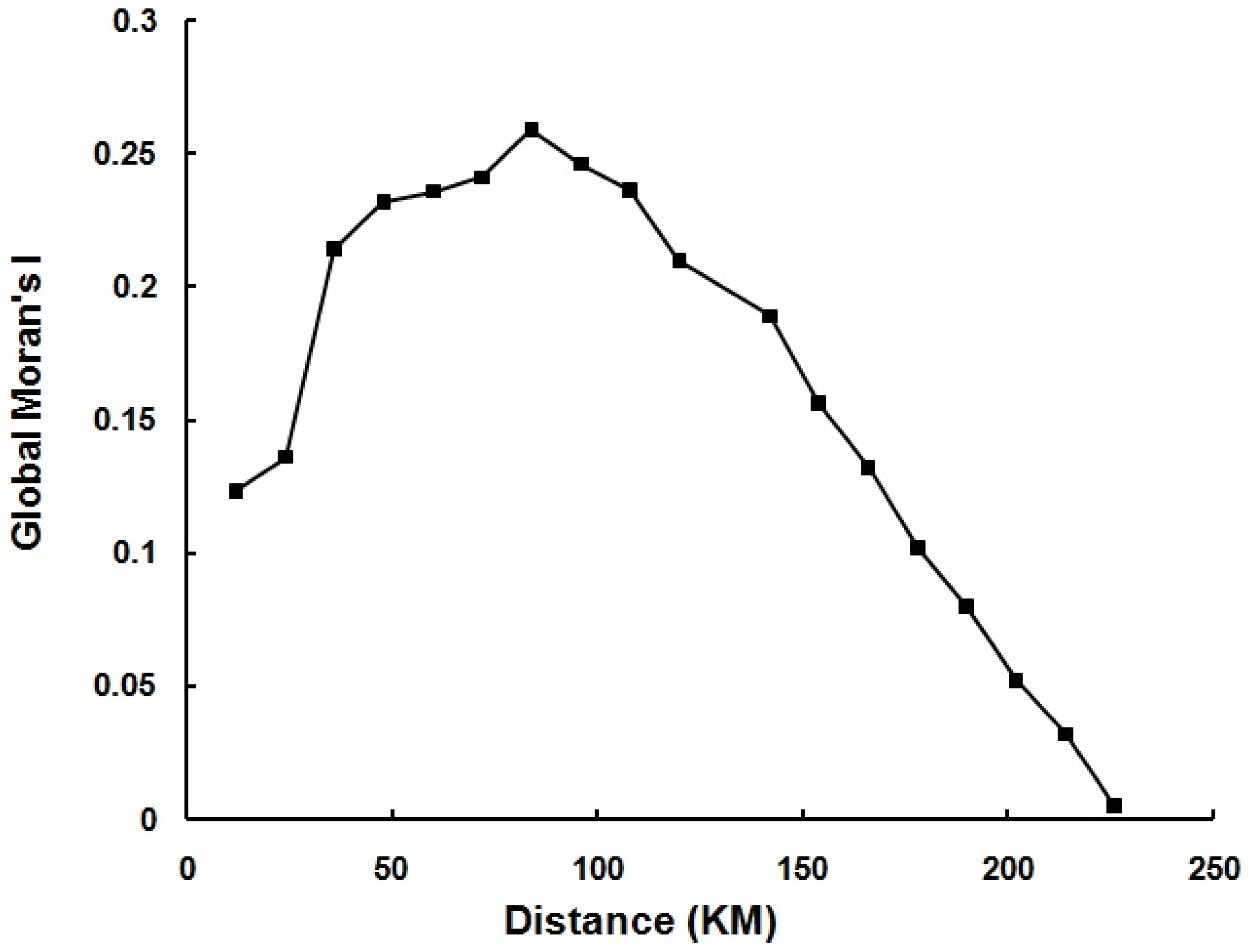
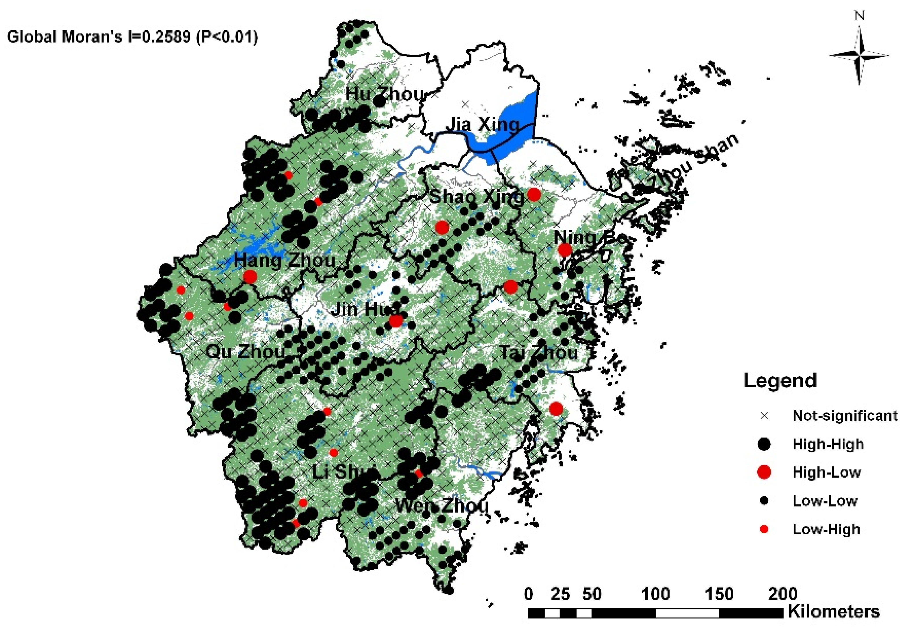
3.4. Spatial-Cluster and Spatial-Outlier Analyses

The plot of global Moran’s I against the distance classes is called a spatial correlogram [44], which can be used to describe the spatial autocorrelation of the studied variables. The spatial correlogram for FBC is shown in Figure 5. The spatial correlogram initially displayed strong spatial dependence (high global Moran’s I value, P < 0.05) when the distance extended to include more FBC values. After reaching the peak (82.3 km), the spatial dependence decreased when the distance further increased. The maximal spatial positive correlation range of the spatial correlogram was about 230 km, where the global Moran’s I value of 0 appears. GIS mapping techniques can help to identify spatial patterns visually, but not statistically [45]. The general spatial variations identified visually based on raw data in Figure 3 can be statistically supported using local Moran’s I method. The results of LISA analysis under the strongest global Moran’s I value (0.2589, P < 0.01) are illustrated in Figure 6.

Figure 5. Spatial correlogram of FBC.

Figure 5. Spatial correlogram of FBC.

Figure 6. Spatial clusters and spatial outliers map of FBC density.

Figure 6. Spatial clusters and spatial outliers map of FBC density.

The results for the majority of FBC density values were not significant. Clear high-high spatial-clusters were observed in the northwestern and southwestern parts of Zhejiang province, mainly along the Tianmu Mountain Area and Lishui Region, respectively. Tianmu Mountain is famous as the main natural conservation area in China, and human being interruption has been forbidden in this area since 1992. Lishui City is a typical mountainous area in Zhejiang Province. Local government has paid a lot of attention to protect the natural resources to improve ecological values. Some low-low spatial-clusters were found in the middle part and southeastern coastal area of study area. Most of the high-low outliers were close to the low-low area. These samples collected from the plots with longer forest ages, had much higher FBC density values than those in the neighborhood. On the other hand, the low-high outliers were mainly located closely to the high-high spatial-cluster area. The most low-high outlier plots have low elevation and receive more interruption by human beings. It should be noticed that the local Moran’s I index is sensitive to outliers [1]. A total of 17 spatial outliers were detected.

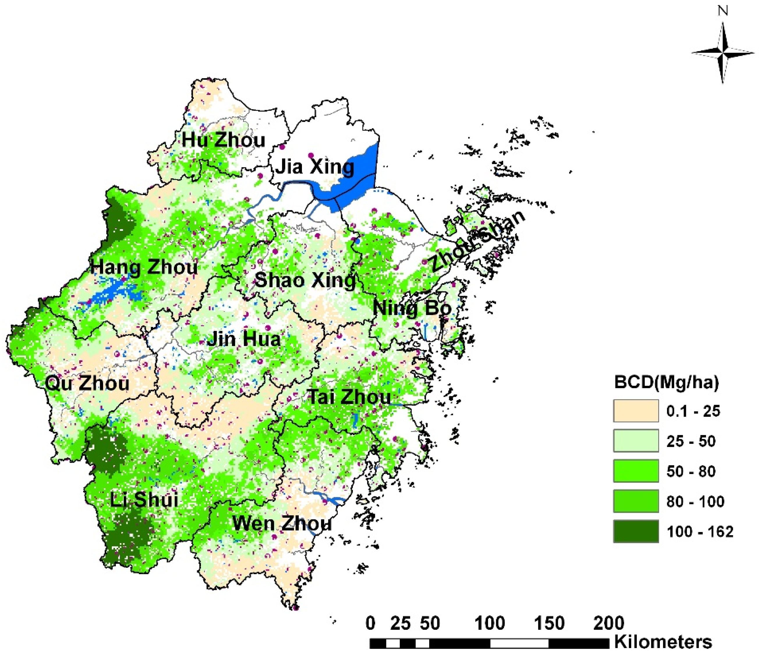
3.5. Semivariance Analysis and Spatial Distribution

To stabilize the spatial variance, the transformed data, excluding the spatial outliers, were used. There was no evident anisotropy in the variogram for Box-Cox transformed data. This meant that the FBC density varied similarly in all directions of the study area and the semivariance depended only on the distance between samples [46]. The best-fit theoretical variogram model for FBC density was chosen based on the highest coefficient values (R²). Compared to other models, a spherical model with the highest R² value was applied for further kriging interpolation (Table 3). The “nugget-to-sill” value was 0.478, indicating a moderate spatial dependence [40]. Both intrinsic and extrinsic factors influenced the spatial dependence of FBC density. The range value was 98.5 km. In geostatistics, the range is the maximum distance between correlated measurements [47]. This range of spatial autocorrelation of FBC density was much greater than the sampling interval, implying that current sampling density was appropriate to study the spatial structure of FBC density in Zhejiang Province.

Table 3. Theoretical semivariogram model and the corresponding parameters for forest biomass carbon density.

Data	Models	(Nugget) C0	(Sill) C0 + C	(Nugget / Sill %) C0/(C0 + C)	Range a (km)	R2
Box-Cox transformation	Spherical	0.011	0.023	47.8	98.5	0.906
	Exponential	0.014	0.024	58.3	102.4	0.875
	Circular	0.018	0.025	72.0	96.3	0.822
	Gaussian	0.021	0.028	75.0	99.7	0.786

Table 3. Theoretical semivariogram model and the corresponding parameters for forest biomass carbon density.

Data	Models	(Nugget) C0	(Sill) C0 + C	(Nugget / Sill %) C0/(C0 + C)	Range a (km)	R2
Box-Cox transformation	Spherical	0.011	0.023	47.8	98.5	0.906
	Exponential	0.014	0.024	58.3	102.4	0.875
	Circular	0.018	0.025	72.0	96.3	0.822
	Gaussian	0.021	0.028	75.0	99.7	0.786

The spatial distribution map produced by trans-Gaussian kriging [48] is shown in Figure 7. In the southwestern part of Zhejiang province, the FBC density values ranged from 80 to 162 Mg ha⁻¹, which were much higher than other areas, while the FBC density was low in the northern part of study area, Hang-Jia-Hu (HJH) Plain, which has little forest. According to the Zhejiang forest inventory report [28], the forest area only accounted for 9.18% of the HJH Plain Area. In the middle part of Zhejiang province (Jin-Qu basin), the FBC values ranged from 0.1 to 50 Mg ha⁻¹. The relatively low FBC values were mainly due to the land management in this area. Jin-Qu Basin is the main commercial grain base. The main forest type is economic forest, which is influenced by human activities. The medium FBC values in the Wenzhou-Taizhou boundary were related to the Yandang Mountain, which is a famous tourist area, while low FBC values were located in the coastal part of southern Zhejiang. The low forest biomass is most likely related to typhoon, climate and human disturbance [43]. These high and low value patterns were in line with the above spatial clusters revealed by local Moran’s I.

Geostatistical methods are important to visually describe the spatial distribution patterns of the variance, which can only be roughly characterized by descriptive statistics [1]. Sampling size and strategy played a vital role in geostatistical analysis. The sample size used in this study was good enough to reveal clear spatial patterns in the kriged interpolation map of FBC density (Figure 7). Most sampling studies indicate that grid sampling provides excellent information of environmental variables when a small grid size is used; important attributes are missed when grid size is increased [49]. Thus, more samples may be necessary to reveal local spatial variation of FBC density in forests, using complex geostatistical analysis such as regression kriging. On the other hand, costs and labor associated with a dense sampling are high; in that case, suitable ancillary data, such as aerial photographs, elevation, forest type map, etc. can be used to study spatial pattern of FBC density.

Figure 7. Spatial distribution map of FBC density.

Figure 7. Spatial distribution map of FBC density.

4. Conclusions

The average FBC density was 27.33 Mg ha⁻¹ in this study. Forest age, forest litter, elevation, soil organic carbon and soil available N were significantly correlated with FBC density. Compared to other typical subtropical forest types, broad-leaved forest had the highest average FBC density, while economical forest had the lowest FBC density. Forest management played an important role in the carbon storage of forest biomass. Moderate spatial dependency was found for FBC density. These results indicate considerable clustering at the 50–100 km size. The spatial variation of FBC density was related to natural and anthropogenic factors.

References

1. Fu, W.J.; Jiang, P.K.; Zhao, K.L.; Zhou, G.M.; Li, Y.F.; Wu, J.S.; Du, H.Q. The carbon storage in moso bamboo plantation and its spatial variation in Anji county of southeastern China. J. Soils Sediments 2014, 14, 320–329. [Google Scholar] [CrossRef]
2. Matysek, A.; Ford, M.; Jakeman, G.; Curtotti, R.; Schneider, K.; Aham-mad, H.; Fisher, B.S. Near Zero Emissions Technologies; ABARE eReport, 05.1; Australian Bureau of Agri-cultural and Resource Economics: Canberra, Australia, 2005. [Google Scholar]
3. Stern, N. The Economics of Climate Change: The Stern Review; Cambridge University Press: Cambridge, UK, 2007. [Google Scholar]
4. IPCC (Intergovernmental Panel on Climate Change). Summary for policymakers: Land use, land-use change, and forestry. In A Special Report of the Intergovernmental Panel on Climate Change; Watson, R.T., Nobel, I.R., Bolin, B., Ravinddranath, N.H., Verardo, D.J., Dokken, D.J., Eds.; Cambridge University Press: Cambridge, UK, 2000; pp. 4–14. [Google Scholar]
5. FAO. Global Ecological Zoning for the Global Forest Resources Assessment; FAO: Rome, Italy, 2000. [Google Scholar]
6. Pan, Y.; Birdsey, R.A.; Fang, J.; Houghton, R.; Kauppi, P.E.; Kurz, W.A.; Phillips, O.L.; Shvidenko, A.; Lewis, S.L.; Canadell, J.G.; et al. A large and persistent carbon sink in the world’s forests. Science 2011, 333, 988–993. [Google Scholar] [CrossRef] [PubMed]
7. Watson, A.J.; Bakker, D.C.E.; Ridgwell, A.J.; Boyd, P.W.; Law, C.S. Effect of iro supply on southern ocean CO2 uptake and implications for glacial atmospheric CO2. Nature 2000, 407, 730–733. [Google Scholar] [CrossRef] [PubMed]
8. Brown, S.L.; Schroeder, P.E. Spatial patterns of aboveground production and mortality of woody biomass for eastern U.S. forests. Ecol. Appl. 1999, 9, 968–980. [Google Scholar]
9. Takahashi, M.; Ishizuka, S.; Ugawa, S.; Sakai, Y.; Sakai, H.; Ono, K.; Morisada, K. Carbon stock in litter, deadwood and soil in Japan’s forest sector and its comparison with carbon stock in agricultural soils. Soil Sci. Plant Nutr. 2010, 56, 19–30. [Google Scholar] [CrossRef]
10. Piao, S.; Fang, J.; Zhu, B.; Tan, K. Forest biomass carbon stocks in China over the past 2 decades: Estimation based on integrated inventory and satellite data. J. Geophys. Res. 2005, 110, G01006. [Google Scholar] [CrossRef]
11. Davis, M.R.; Allen, R.B.; Clinton, P.W. Carbon storage along a stand development sequence in a New Zealand Nothofagus forest. For. Ecol. Manag. 2003, 177, 313–321. [Google Scholar] [CrossRef]
12. Fang, J.; Chen, A.; Peng, C.; Zhao, S.; Ci, L. Changes in forest biomass carbon storage in China between 1949 and 1998. Science 2001, 292, 2320–2322. [Google Scholar] [CrossRef] [PubMed]
13. Hazlett, P.W.; Gordon, A.M.; Sibley, P.K.; Buttle, J.M. Stand carbon stocks and soil carbon and nitrogen storage for riparian and upland forests of boreal lakes in northeastern Ontario. For. Ecol. Manag. 2005, 219, 56–68. [Google Scholar] [CrossRef]
14. Fang, J.; Guo, Z.; Piao, S.; Chen, A. Terrestrial vegetation carbon sinks in China, 1981–2000. Sci. China Ser. D Earth Sci. 2007, 50, 1341–1350. [Google Scholar] [CrossRef]
15. Xu, X.L.; Cao, M.K.; Li, K.R. Temporal-spatial dynamics of carbon storage of forest vegetation in China. Prog. Geog. 2007, 27, 1–10. [Google Scholar]
16. Guo, Z.; Fang, J.; Pan, Y.; Birdsey, R. Inventory-based estimates of forest biomass carbon stocks in China: A comparison of three methods. For. Ecol. Manag. 2010, 259, 1225–1231. [Google Scholar] [CrossRef]
17. Du, L.; Zhou, T.; Zou, Z.; Zhao, X.; Huang, K.; Wu, H. Mapping forest biomass using remote sensing and national forest inventory in China. Forests 2014, 5, 1267–1283. [Google Scholar] [CrossRef]
18. Jeffrey, Q.C.; Robinson, N.J.; Daniel, M.M.; Alan, D.V.; Joerg, T.; Dar, R.; Gabriel, H.; Susan, T.; Niro, H. The steady-state mosaic of disturbance and succession across an old-growth central amazon forest landscape. Proc. Nat. Acad. Sci. 2013, 110, 3949–3954. [Google Scholar]
19. Wang, Y.Q.; Zhang, X.C.; Zhang, J.L.; Li, S.J. Spatial variability of soil organic carbon in a watershed on the Loess Plateau. Pedosphere 2009, 19, 486–495. [Google Scholar] [CrossRef]
20. Vittorio, A.; Negron-Juarez, R.; Higuchi, N.; Chambers, J. Tropical forest carbon balance: Effects of field- and satellite-based mortality regimes on the dynamics and the spatial structure of central amazon forest biomass. Environ. Res. Lett. 2014, 9, 034010. [Google Scholar] [CrossRef]
21. Du, H.Q.; Zhou, G.M.; Fan, W.Y.; Ge, H.L.; Xu, X.J.; Shi, Y.J.; Fan, W.L. Spatial heterogeneity and carbon contribution of aboveground biomass of moso bamboo by using geostatistical theory. Plant Ecol. 2010, 207, 131–139. [Google Scholar] [CrossRef]
22. Chen, X.G.; Zhang, X.Q.; Zhang, Y.P.; Booth, T.; He, X.H. Changes of carbon stocks in bamboo stands in China 100 years. For. Ecol. Manag. 2009, 258, 1489–1496. [Google Scholar] [CrossRef]
23. Wang, Z.Q. Geostatistics and Its Application in Ecology; Science Press: Beijing, China, 1999. [Google Scholar]
24. FAO. Global Forest Resource Assessment 2005; Food and Agricultural Organization of the United Nations: Rome, Italy, 2006. [Google Scholar]
25. Zhejiang Forestry Bureau. Forest Resources in Zhejiang Province; China Agricultural and Technological Press: Beijing, China, 2006; pp. 5–9. (In Chinese) [Google Scholar]
26. Yuan, W.G.; Shen, A.H.; Jiang, B.; Zhu, J.R.; Lu, G. Study on litterfall characteristics of evergreen broadleaf forest in Zhejiang. J. Zhejiang For. Sci. Technol. 2009, 29, 1–4. (In Chinese) [Google Scholar]
27. Webster, R.; Oliver, M.A. Geostatistics for Environmental Scientists; John Wiley & Sons: Hoboken, NJ, USA, 2007. [Google Scholar]
28. Moran, P.A. Notes on continuous stochastic phenomena. Biometrika 1950, 37, 17–23. [Google Scholar] [CrossRef] [PubMed]
29. Tu, J.; Xia, Z.G. Examining spatially varying relationships between land use and water quality using geographically weighted regression I: Model design and evaluation. Sci. Total Environ. 2008, 407, 358–378. [Google Scholar] [CrossRef] [PubMed]
30. Anselin, L. Local indicators of spatial association—LISA. Geogr. Anal. 1995, 27, 93–115. [Google Scholar] [CrossRef]
31. Anselin, L. Andy Isserman’s Regional Science. Int. Reg. Science Rev. 2013, 36, 4–15. [Google Scholar] [CrossRef]
32. Zhang, C.S.; Luo, L.; Xu, W.; Ledwith, V. Use of local Moran’s I and GIS to identify pollution hotspots of Pb in urban soils of Galway, Ireland. Sci. Total Environ. 2008, 398, 212–221. [Google Scholar] [CrossRef] [PubMed]
33. Levine, N. CrimeStat III: A Spatial Statistics Program for the Analysis of Crime Incident Locations; Ned Levine & Associates: Houston, TX, USA; The National Institute of Justice: Washington, DC, USA, 2004. [Google Scholar]
34. Goovaerts, P. Geostatistics for Natural Resources Evaluation; Oxford University Press: New York, NY, USA, 1997. [Google Scholar]
35. Huang, C.D.; Zhang, J.; Yang, W.Q.; Tang, X. Spatial-temporal variation of carbon storage in forest vegetation in Sichuan Province. Chin. J. Appl. Ecol. 2007, 18, 2687–2692. [Google Scholar]
36. Wang, Y.X. Carbon Stock of Main Forest Types in Fujian Province and Carbon Sequestration of Cunninghamis Lanceolata Plantation; Fujian Agriculture and Forest University: Fujian, China, 2004. [Google Scholar]
37. Cao, J.; Zhang, Y.L.; Liu, Y.H. Changes in forest biomass carbon storage in Hainan Island over the last 20 years. Geogr. Res. 2002, 21, 551–560. [Google Scholar]
38. Liu, C.; Zhang, L.J.; Li, F.L.; Jin, X.J. Spatial modeling of the carbon stock of forest trees in Heilongjiang Province China. J. For. Res. 2014, 25, 269–280. [Google Scholar] [CrossRef]
39. Zhang, F.; Du, Q.; Ge, H.L.; Liu, A.X.; Fu, W.J.; Ji, B.Y. Spatial distribution of forest carbon in Zhejiang Province with geostatistics based on CFI sample plots. Acta Ecol. Sin. 2012, 32, 5275–5286. (In Chinese) [Google Scholar] [CrossRef]
40. Zhang, X.Y.; Sui, Y.Y.; Zhang, X.D.; Meng, K.; Herbert, S.J. Spatial variability of nutrient properties in black soil of northeast China. Pedosphere 2007, 17, 19–29. [Google Scholar] [CrossRef]
41. Chang, J.; Clay, D.E.; Carlson, C.G.; Clay, S.A.; Malo, D.D.; Berg, R.; Wiebold, W. Different techniques to identify management zones impact nitrogen and phosphorus sampling variability. Agron. J. 2003, 95, 1550–1559. [Google Scholar] [CrossRef]
42. Cao, F.Q.; Liu, C.H.; Liu, M.; Cui, J.F. Guangxi agricultural sciences. G.X. Agric. Sci. 2010, 41, 693–697. (In Chinese) [Google Scholar]
43. Huang, C.C.; Ge, Y.; Zhu, J.R.; Yuan, W.G.; Qi, L.Z.; Jiang, B.; Chang, J. The litter of Pinus massoniana ecological public-welfare forest in Zhejiang Province and its relationship with the community characters. Acta Ecol. Sin. 2005, 25, 2507–2513. [Google Scholar]
44. Overmars, K.P.; de Koning, G.H.J.; Veldkamp, A. Spatial autocorrelation in multi-scale land use models. Ecol. Model. 2003, 164, 257–270. [Google Scholar] [CrossRef]
45. Cambardella, C.A.; Moorman, A.T.; Novak, J.M.; Parkin, T.B.; Karlen, D.L.; Turco, R.F.; Konopka, A.E. Field-scale variability of soil properties in central Iowa soils. Soil Sci. Soc. Am. J. 1994, 58, 1501–1511. [Google Scholar] [CrossRef]
46. Fu, W.J.; Tunney, H.; Zhang, C.S. Spatial variation of soil test phosohorus in a long-term grazed experimental grassland field. J. Plant Nutr. Soil Sci. 2010, 173, 323–331. [Google Scholar]
47. Utset, A.; Ruiz, M.E.; Herrera, J.; de Leon, D.P. A geostatistical method for soil salinity sample site spacing. Geoderma 1998, 86, 143–175. [Google Scholar] [CrossRef]
48. Cressie, N. Statistics for Spatial Data, Revised ed.; John Wiley: Hoboken, NJ, USA, 1993. [Google Scholar]
49. Mallarino, A.P.; Wittry, D.J. Efficacy of grid and zone soil sampling approaches for site-specific assessment of phosphorus, potassium, pH and organic matter. Precis. Agric. 2004, 5, 131–144. [Google Scholar] [CrossRef]