
Spatial Forest Harvest Scheduling for Areas Involving Carbon and Timber Management Goals


Abstract
:1. Introduction
2. Materials

3. Methods
3.1. Forest Growth and Yield Models
3.2. Forest Planning Formulation
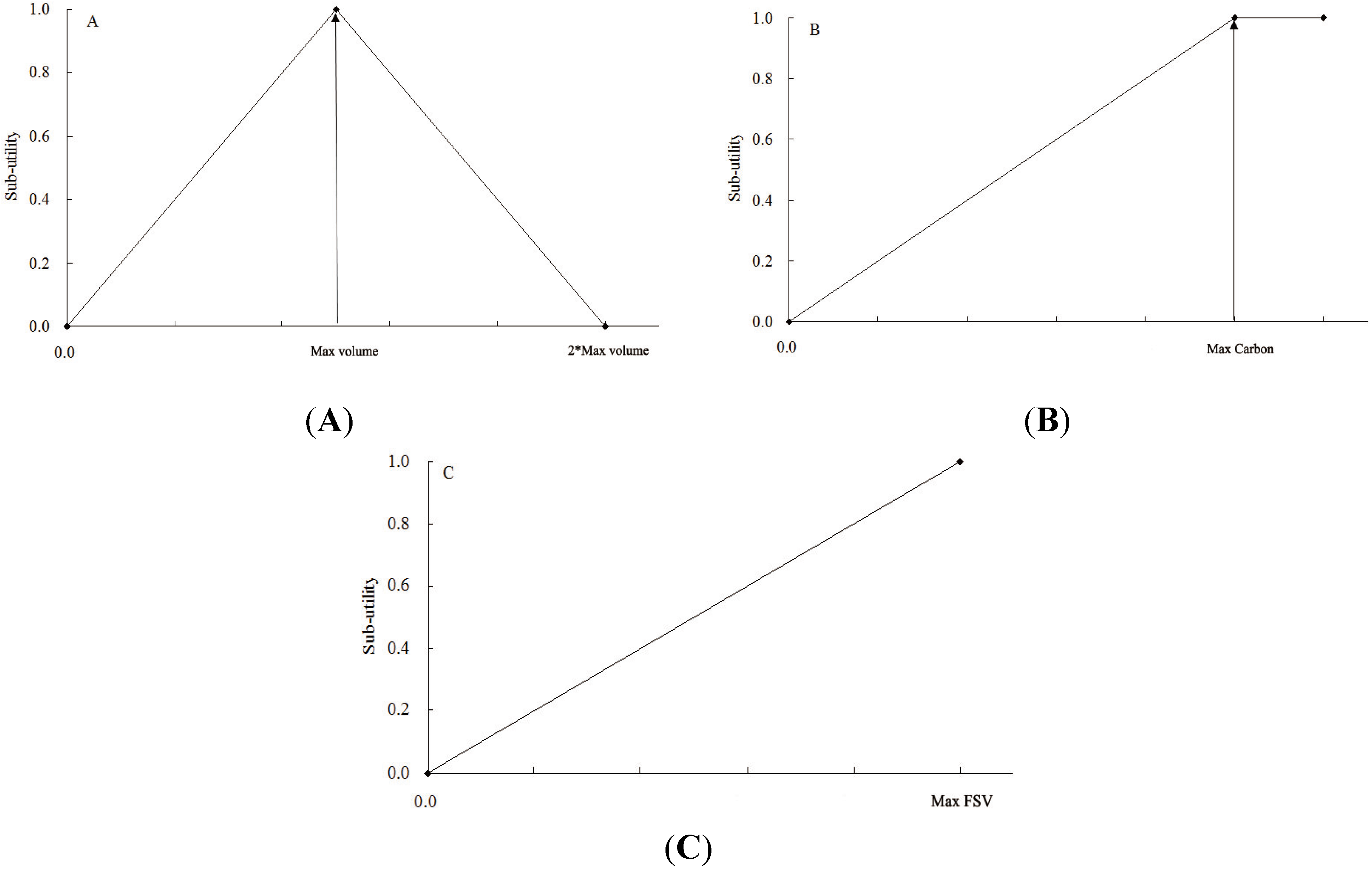
3.2.1. Objective Function

3.2.2. Constraints
3.2.3. Management Activities
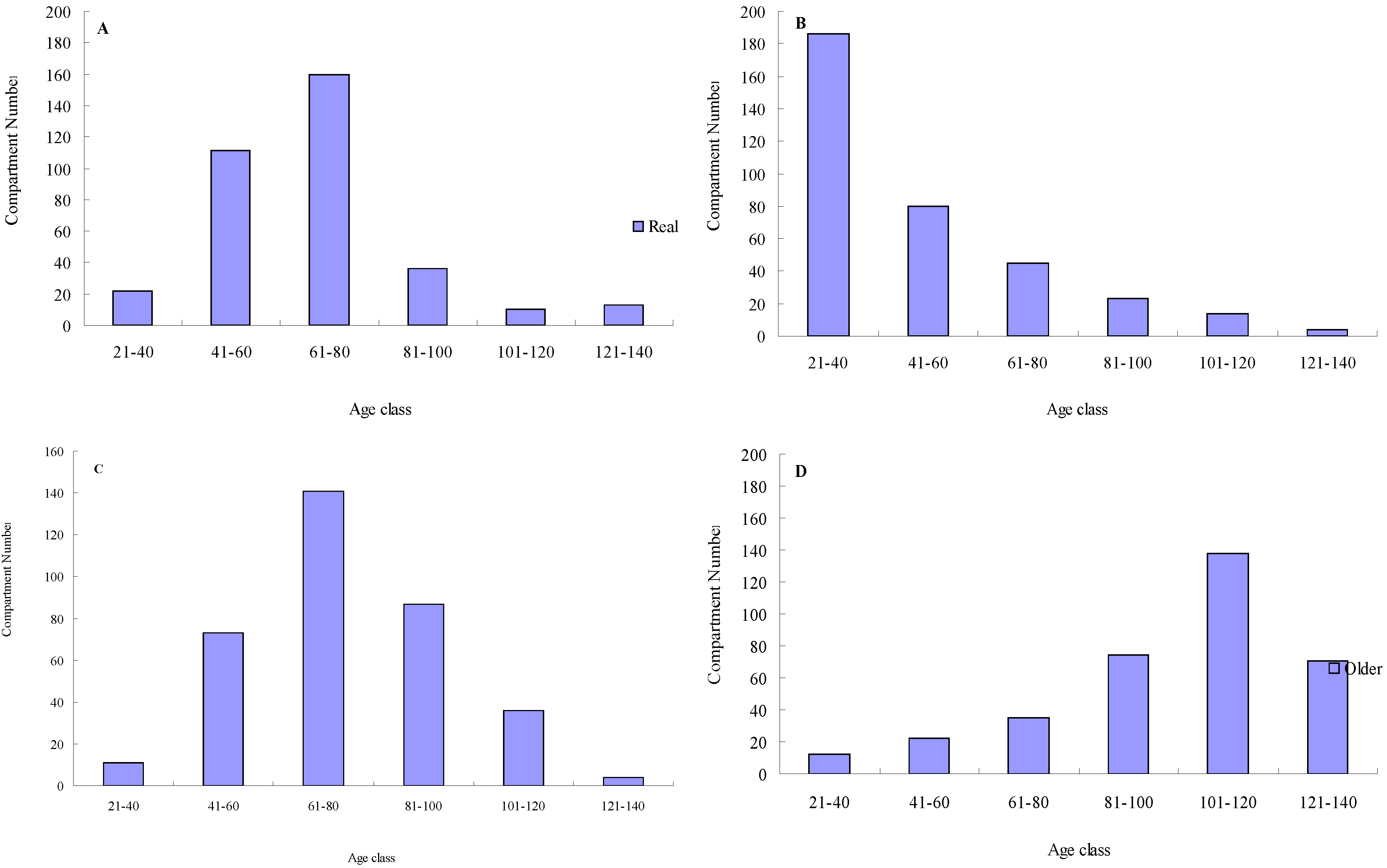
3.3. Evaluation of Different Age Class Distributions
3.4. Heuristic Search Algorithm
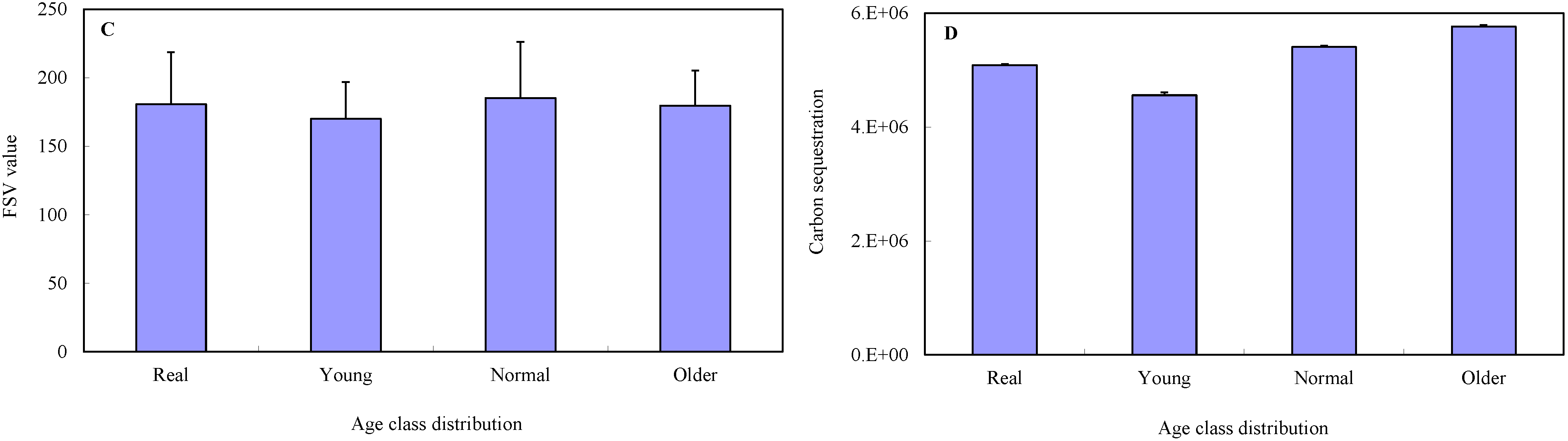
4. Results

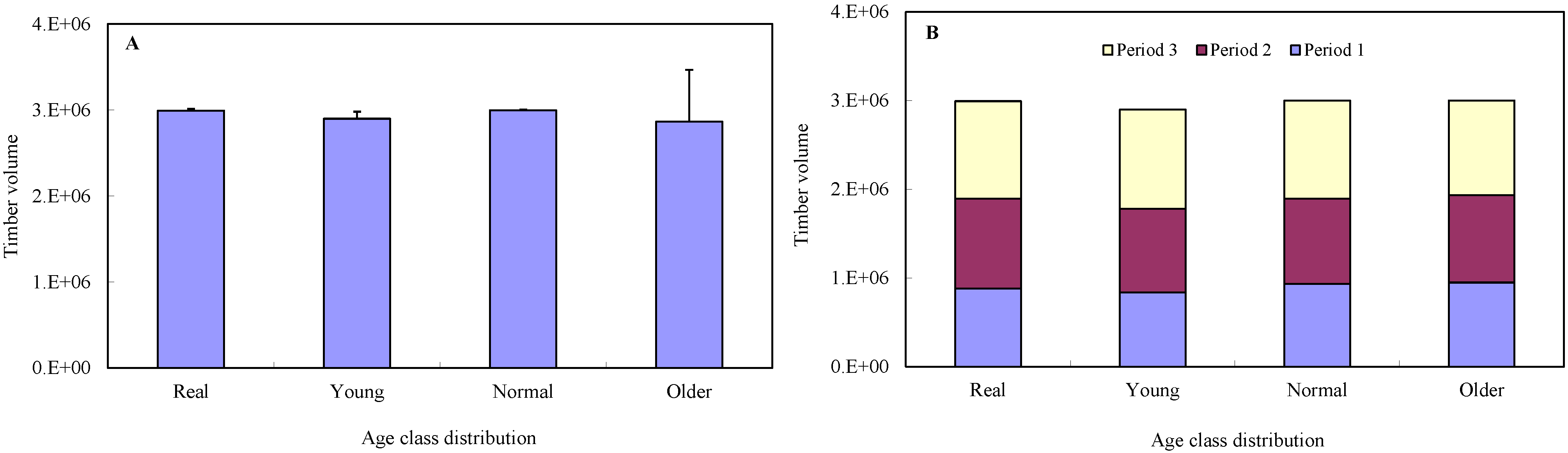
| Forest Scenario | Solution Value | Computing Time | ||||
|---|---|---|---|---|---|---|
| Min. | Max. | Mean | SD | Mean (min) | SD (min) | |
| Actual | 0.6146 | 0.6253 | 0.6209 | 0.0027 | 4.6417 | 1.6804 |
| Young | 0.5661 | 0.5927 | 0.5809 | 0.0078 | 37.0208 | 16.2809 |
| Normal | 0.6329 | 0.6468 | 0.6392 | 0.0025 | 2.9792 | 0.9740 |
| Older | 0.6572 | 0.6623 | 0.6594 | 0.0013 | 2.4483 | 0.7038 |


5. Discussion
6. Conclusions
Acknowledgments
Author Contributions
Conflicts of Interest
References
- Kyoto Protocol to the United Nations framework convention on climate change. Available online: http://unfccc.int/resource/docs/convkp/kpeng.pdf (accessed on 9 February 2015).
- Neilson, E.T.; MacLean, D.A.; Meng, F.R.; Arp, P.A. Spatial distribution of carbon in natural and management stands in an industrial forest in New Brunswick, Canada. For. Ecol. Manag. 2007, 253, 148–160. [Google Scholar] [CrossRef]
- Malhi, Y.; Aragão, L.O.C.; Metcalfe, D.B.; Paiva, R.; Quesada, C.A.; Almeida, S.; Anderson, L.; Brando, P.; Chambers, J.Q.; Dacosta, A.C.L.; et al. Comprehensive assessment of carbon productivity, allocation and storage in three Amazonian forest. Glob. Chang. Biol. 2009, 15, 1255–1274. [Google Scholar] [CrossRef]
- Pan, Y.D.; Birdsey, R.A.; Fang, J.Y.; Houghton, R.; Kauppi, P.E.; Kurz, W.A.; Phillips, O.L.; Shvidenko, A.; Lewis, S.L.; Canadell, J.G.; et al. A large and persistent carbon sink in the world’s forests. Science 2011, 333, 988–992. [Google Scholar] [CrossRef] [PubMed]
- Joosten, R.; Schumacher, J.; Wirth, C.; Schulte, A. Evaluating tree carbon predictions for beech (Fagus sylvatica L.) in western Germany. For. Ecol. Manag. 2004, 189, 87–96. [Google Scholar] [CrossRef]
- Guo, Z.D.; Fang, J.Y.; Pan, Y.D.; Birdsey, R. Inventory-based estimates of forest biomass carbon stocks in China: A comparison of three methods. For. Ecol. Manag. 2010, 259, 1225–1231. [Google Scholar] [CrossRef]
- Grote, R.; Kiese, R.; Grünwald, T.; Ourcival, J.M.; Granier, A. Modelling forest carbon balances considering tree morality and removal. Agric. For. Meteorol. 2011, 151, 179–190. [Google Scholar] [CrossRef]
- Finkral, A.J.; Evans, A.M. The effects of a thinning treatment on carbon stocks in a northern Arizona ponderosa pine forest. For. Ecol. Manag. 2008, 255, 2743–2750. [Google Scholar] [CrossRef]
- Thùrig, E.; Kaufmann, E. Increasing carbon sinks through forest management: A model-based comparison for Switzerland with its Eastern Plateau and Eastern Alps. Eur. J. For. Res. 2010, 129, 563–572. [Google Scholar] [CrossRef]
- Powers, M.; Kolka, R.; Palik, B.; McDonald, R.; Jurgensen, M. Long-term management impacts on carbon storage in Lake States forests. For. Ecol. Manag. 2011, 262, 424–431. [Google Scholar] [CrossRef]
- Manusch, C.; Bugmann, H.; Wolf, A. The impact of climate change and its uncertainty on carbon storage in Switzerland. Reg. Environ. Chang. 2014, 14, 1437–1450. [Google Scholar] [CrossRef]
- Selmants, P.C.; Litton, C.M.; Giardina, C.P.; Asner, G.P. Ecosystem carbon storage does not vary with mean annual temperature in Hawaiian tropical montage wet forests. Glob. Chang. Biol. 2014, 20, 2927–2937. [Google Scholar] [CrossRef] [PubMed]
- Lal, R. Forest soils and carbon sequestration. For. Ecol. Manag. 2005, 220, 242–258. [Google Scholar] [CrossRef]
- Ter-Mikaelian, M.T.; Colombo, S.J.; Chen, J. The burning question: Does forest bioenergy reduce carbon emissions? A review of common misconceptions about forest carbon accounting. J. For. 2015, 113, 57–68. [Google Scholar]
- Liski, J.; Pussinen, A.; Pingoud, K.; Mäkipää, R.; Karjalainen, T. Which rotation length is favorable to carbon sequestration? Can. J. For. Res. 2001, 31, 2004–2013. [Google Scholar] [CrossRef]
- Seely, B.; Welham, C.; Kimmins, H. Carbon sequestration in a boreal forest ecosystem: Results from the ecosystem simulation model, FORECAST. For. Ecol. Manag. 2002, 169, 123–135. [Google Scholar] [CrossRef]
- Daust, D.K.; Nelson, J.D. Spatial reduction factors for strata-based harvest schedules. For. Sci. 1993, 39, 152–165. [Google Scholar]
- Boston, K.; Bettinger, P. The economic impact of green-up constraints in the southeastern United States. For. Ecol. Manag. 2001, 191–202. [Google Scholar] [CrossRef]
- Nalle, D.; Arthur, J.L.; Montgomery, C.A. Economic impacts of adjacency and green-up constraints on timber production at a landscape scale. J. For. Econ. 2005, 10, 189–205. [Google Scholar]
- Bennett, E.M.; Peterson, G.D.; Gordon, L.J. Understanding relationships among multiple ecosystem services. Ecol. Lett. 2009, 12, 1394–1404. [Google Scholar] [CrossRef] [PubMed]
- Cademus, R.; Escobedo, F.J.; McLaughlin, D.; Abd-Elrhman, A. Analyzing trade-offs, synergies, and drivers among timber production, carbon sequestration, and water yield in Pinus elliotii forests in southeastern USA. Forests 2014, 5, 1409–1431. [Google Scholar] [CrossRef]
- Bettinger, P.; Chung, W. The key literature of, and trends in, forest-level management planning in north America, 1950–2001. Int. For. Rev. 2004, 6, 40–50. [Google Scholar]
- Meng, F.R.; Bourque, C.P.A.; Oldford, S.P.; Swift, D.E.; Smith, H.C. Combining carbon sequestration objectives with timber management planning. Mitig. Adapt. Strat. Glob. Chang. 2003, 8, 371–403. [Google Scholar] [CrossRef]
- Backéus, S.; Wikström, P.; Lämås, T. A model for regional analysis of carbon sequestration and timber production. For. Ecol. Manag. 2005, 216, 28–40. [Google Scholar] [CrossRef]
- Bourque, C.P.A.; Neilson, E.T.; Gruenwald, C.; Perrin, S.F.; Hiltz, J.C.; Blin, Y.A.; Horsman, G.V.; Parker, M.S.; Thorburn, C.B.; Corey, M.M.; et al. Optimizing carbon sequestration in commercial forests by integrating carbon management objectives in wood supply modeling. Mitig. Adapt. Strat. Glob. Chang. 2007, 12, 1253–1275. [Google Scholar] [CrossRef]
- Hennigar, C.R.; MacLean, D.A.; Amos-Binks, L.J. A novel approach to optimize management strategies for carbon stored in both forest and wood products. For. Ecol. Manag. 2008, 256, 786–797. [Google Scholar] [CrossRef]
- Öhman, K.; Lämås, T. Clustering of harvest activities in multi-objective long-term forest planning. For. Ecol. Manag. 2003, 176, 161–171. [Google Scholar] [CrossRef]
- Rempel, R.S.; Kaufmann, C.K. Spatial modeling of harvest constraints on wood supply versus wildlife habitat objectives. Environ. Manag. 2003, 32, 646–659. [Google Scholar] [CrossRef]
- Bettinger, P.; Boston, K.; Kim, Y.H.; Zhu, J.P. Landscape-level optimization using tabu search and stand density-related forest management prescriptions. Eur. J. Oper. Res. 2007, 176, 1265–1282. [Google Scholar] [CrossRef]
- Lu, F.D.; Eriksson, L.O. Formation of harvest units with genetic algorithms. For. Ecol. Manag. 2000, 130, 57–67. [Google Scholar] [CrossRef]
- Bettinger, P.; Johnson, D.L.; Johnson, K.N. Spatial forest plan development with ecological and economic goals. Ecol. Mod. 2003, 169, 215–236. [Google Scholar] [CrossRef]
- Bettinger, P.; Graetz, D.; Boston, K.; Sessions, J.; Chung, W. Eight heuristic planning techniques applied to three increasingly difficult wildlife planning problems. Silva Fenn. 2002, 36, 561–584. [Google Scholar] [CrossRef]
- Li, R.X.; Bettinger, P.; Boston, K. Informed development of meta heuristics for spatial forest planning problems. Open Oper. J. 2010, 4, 1–11. [Google Scholar] [CrossRef]
- Čavlović, J.; Antonić, O.; Božić, M.; Teslak, K. Long-term and country scale projection of even-aged forest management: A case study for Fagus sylvatica in Croatia. Scand. J. For. Res. 2012, 27, 36–45. [Google Scholar] [CrossRef]
- Chen, Y.T.; Zheng, C.; Chang, C.T. Efficiently mapping an appropriate thinning schedule for optimum carbon sequestration: An application of multi-segment goal programming. For. Ecol. Manag. 2011, 262, 1168–1173. [Google Scholar] [CrossRef]
- Dong, L.H.; Li, F.R.; Jia, W.W.; Liu, F.X.; Wang, H.Z. Compatible biomass models for main tree species with measurement error in Heilongjiang Province of Northeast China. Chin. J. Appl. Ecol. 2011, 22, 2653–2661. [Google Scholar]
- Wang, H.Z. Dynamic Simulating System for Stand Growth of Forests in Northeast China. Ph.D. Thesis, Northeast Forestry University, Harbin, China, 2012. [Google Scholar]
- Pukkala, T.; Ketonen, T.; Pykäläinen, J. Predicting timber harvests from private forest-a utility maximization approach. For. Policy Econ. 2003, 5, 285–296. [Google Scholar] [CrossRef]
- Chen, B.W.; Gadow, K.V. Timber harvest planning with spatial objectives, using the method of simulated annealing. Eur. J. For. Res. 2002, 121, 25–34. [Google Scholar]
- Bettinger, P. A prototype method for integrating spatially-referenced wildfires into a tactical forest planning model. Res. J. For. 2009, 3, 8–22. [Google Scholar]
- Barrett, T.M.; Gilless, J.K.; Davis, L.S. Economic and fragmentation effects of clearcut restrictions. For. Sci. 1998, 44, 569–577. [Google Scholar]
- Bettinger, P.; Sessions, J.; Johnson, K.N. Ensuring the compatibility of aquatic habitat and commodity production goals in eastern Oregon with a Tabu search procedure. For. Sci. 1998, 44, 96–112. [Google Scholar]
- Metropolis, N.; Rosenbluth, A.W.; Rosenbluth, M.N.; Teller, A.H.; Teller, E. Equation of state calculations by fast computing machines. J. Chem. Physics 1953, 21, 1087–1092. [Google Scholar] [CrossRef]
- Boston, K.; Bettinger, P. An analysis of Monte-Carlo integer programming, simulated annealing, and tabu search heuristics for solving spatial harvest scheduling problems. For. Sci. 1999, 45, 292–301. [Google Scholar]
- Öhman, K.; Eriksson, L.O. The core area concept in forming contiguous areas for long-term forest planning. Can. J. For. Res. 1998, 28, 1032–1039. [Google Scholar] [CrossRef]
- Baskent, E.Z.; Jordan, G.A. Forest landscape management modeling using simulated annealing. For. Ecol. Manag. 2002, 165, 29–45. [Google Scholar] [CrossRef]
- Talbi, E.G. Meta-Heuristics. From Design to Implementation; John Wiley & Sons: Hoboken, NJ, USA, 2009. [Google Scholar]
- Pukkala, T.; Heinonen, T. Optimizing heuristic search in forest planning. Nonlinear Anal.: Real World Appl. 2006, 7, 1284–1297. [Google Scholar] [CrossRef]
- Li, H.Q.; Lei, Y.C.; Zeng, W.S. Forest carbon storage in China estimated using forestry inventory data. Sci. Silv. Sin. 2011, 47, 7–12. [Google Scholar]
- Bettinger, P.; Siry, J.; Merry, K. Forest management planning technology issues posed by climate change. For. Sci. Technol. 2013, 9, 9–19. [Google Scholar]
- Jones, D. A practical weight sensitivity algorithm for goal and multiple objective programming. Eur. J. Oper. Res. 2011, 213, 238–245. [Google Scholar] [CrossRef]
- Jadidi, O.; Zolfaghari, S.; Cavalieri, S. A new normalized goal programming model for multi-objective problems: A case of supplier selection and order allocation. Int. J. Prod. Econ. 2014, 148, 158–165. [Google Scholar] [CrossRef]
- Heinonen, T.; Pukkala, T. A comparison of one- and two-compartment neighborhoods in heuristic search with spatial forest management goals. Silva Fenn. 2004, 38, 319–332. [Google Scholar] [CrossRef]
- Öhman, K.; Eriksson, L.O. Allowing for spatial consideration in long-term forest planning by linking linear programming with simulated annealing. For. Ecol. Manag. 2002, 161, 221–230. [Google Scholar] [CrossRef]
- Bettinger, P.; Demirci, M.; Boston, K. Search reversion within s-metaheuristics: Impacts illustrated with a forest planning problem. Silva Fenn. 2015, 49, 1–20. [Google Scholar]
- Jumppanen, J.; Kurttila, M.; Pukkala, T.; Uuttera, J. Spatial harvest scheduling approach for areas involving multiple ownership. For. Policy Econ. 2003, 5, 27–38. [Google Scholar] [CrossRef]
© 2015 by the authors; licensee MDPI, Basel, Switzerland. This article is an open access article distributed under the terms and conditions of the Creative Commons Attribution license (http://creativecommons.org/licenses/by/4.0/).
Share and Cite
Dong, L.; Bettinger, P.; Liu, Z.; Qin, H. Spatial Forest Harvest Scheduling for Areas Involving Carbon and Timber Management Goals. Forests 2015, 6, 1362-1379. https://doi.org/10.3390/f6041362
Dong L, Bettinger P, Liu Z, Qin H. Spatial Forest Harvest Scheduling for Areas Involving Carbon and Timber Management Goals. Forests. 2015; 6(4):1362-1379. https://doi.org/10.3390/f6041362
Chicago/Turabian StyleDong, Lingbo, Pete Bettinger, Zhaogang Liu, and Huiyan Qin. 2015. "Spatial Forest Harvest Scheduling for Areas Involving Carbon and Timber Management Goals" Forests 6, no. 4: 1362-1379. https://doi.org/10.3390/f6041362