
Effect of Planting Density on Knot Attributes and Branch Occlusion of Betula alnoides under Natural Pruning in Southern China

 ,
,
Abstract
:1. Introduction
2. Materials and Methods

| Symbols | Attributes represent | Precision |
|---|---|---|
| Tree attributes | ||
| DBH | Stem diameter at breast height | 0.1 cm |
| HCB | Height of the crown base | 0.1 m |
| CD | Crown diameter | 0.1 m |
| Branch attributes | ||
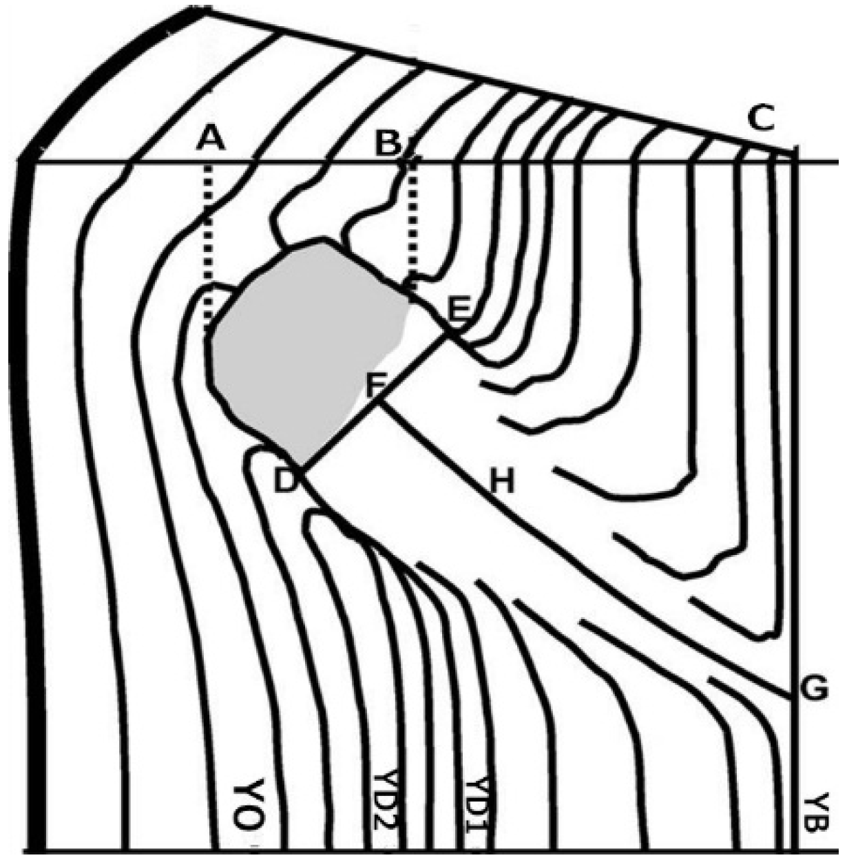
| OT | Time of branch occlusion | 1 year |
| OBD | Diameter of occluded branch | 0.01 mm |
| IA | Insertion angle of the occluded branch | 1° |
| IH | Insertion height of the occluded branch on stem | 0.01 m |
| SDGR | Stem diameter growth rate during the branch occlusion | mm year−1 |
| RLP | Radius of the living portion of knot (live knot) | 0.01 mm |
| RDP | Radius of the dead portion of knot (dead knot) | 0.01 mm |
| TRK | Total radius of knot (RLP + RDP) | 0.01 mm |
| YB | Year of birth of the branch | 1 year |
| YD | Year of death of the branch | 1 year |
| YO | Year of the complete occlusion of the dead branch | 1 year |
| Model descriptors | ||
| a, b, c, d | Coefficients of fixed effect | |
| p, pt, ptb | Subscripts for plot, tree and branch | |
| α, β, γ, δ | Variance components (random effects) | |
| ln() | Symbol for link function in GLMM; here: Log-link | |
| E, |E|, E2 | Mean error, mean absolute error, mean squared error | |
| Φ | Dispersion parameter | |
| Units | ||
| sph | Stems per hectare | |
| Planting Density (sph) | Spacing (Row × Tree) (m) | Tree Height (m) | DBH (cm) | HCB (m) | CD (m) | Basal Area (m2 ha−1) |
|---|---|---|---|---|---|---|
| 3333 | 1.5 × 2 | 13.76 (0.69) a | 14.11 (0.39) c | 8.63 (0.43) a | 2.84 (0.07) b | 20.52 (0.61) a |
| 1667 | 2 × 3 | 14.04 (1.51) a | 14.81 (0.51) b,c | 8.46 (1.26) a | 3.03 (0.19) b | 15.76 (1.46) b |
| 1111 | 3 × 3 | 13.10 (0.60) a | 14.71 (0.33) b,c | 7.27 (0.40) a | 3.47 (0.10) b | 13.02 (0.72) b,c |
| 833 | 3 × 4 | 13.71 (0.60) a | 16.38 (0.45) a,b | 7.40 (1.00) a | 3.35 (0.33) b | 11.09 (1.05) c |
| 500 | 4 × 5 | 13.99 (1.35) a | 17.45 (0.62) a | 6.00 (1.00) a | 4.62 (0.20) a | 7.59 (0.32) d |
3. Results
3.1. Effect of Planting Density on the Time of Branch Occlusion
| Planting Density (sph) | ||||||||||
|---|---|---|---|---|---|---|---|---|---|---|
| 3333 | 1667 | 1111 | 833 | 500 | ||||||
| Min–Max | Mean | Min–Max | Mean | Min–Max | Mean | Min–Max | Mean | Min–Max | Mean | |
| IH | 0.33–14.78 | 6.00 (0.21) a | 0.48–19.72 | 7.23 (0.78) a | 0.26–15.79 | 5.89 (0.24) a | 0.31–16.74 | 6.59 (0.26) a | 0.32–17.92 | 6.10 (0.30) a |
| SDGR | 4.81–40.98 | 13.95 (0.34) a | 4.32–34.75 | 13.12 (0.33) a | 4.85–40.74 | 15.35 (0.44) a | 6.8–38.04 | 15.10 (0.36) a | 5.45–42.94 | 14.28 (0.40) a |
| OT | 1–7 | 1.8 (0.1) b | 1–10 | 2.1 (0.1) a | 1–9 | 2.2 (0.1) a | 1–8 | 2.1 (0.1) a,b | 1–9 | 2.3 (0.1) a |
| OBD | 3.49–29.95 | 10.60 (0.25) c | 3.73–29.63 | 11.77 (0.24) b,c | 2.93–31.91 | 12.4 (0.35) b | 4.74–39.81 | 14.21 (0.43) a | 4.67–55.1 | 14.98 (0.51) a |
| IA | 33–81 | 55.5 (0.5) b | 40–82 | 56.0 (0.4) b | 30–82 | 56.0 (0.5) b | 30–88 | 58.6 (0.6) a | 31–88 | 59.6 (0.9) a |
| RLP | 6.11–64.22 | 25.26 (0.61) c | 4.14–70.97 | 28.47 (0.69) c | 4.58–86.6 | 27.75 (0.99) c | 8.45–96.06 | 33.48 (1.02) b | 4.14–102.29 | 38.8 (1.29) a |
| RDP | 3.23–38.45 | 11.79 (0.33) c | 2.6–51.53 | 13.09 (0.41) b,c | 2.93–70.06 | 16.82 (0.62) a | 1.7–53.22 | 15.05 (0.52) a,b | 3.76–71.05 | 16.75 (0.86) a |
| TRK | 13.37–78.47 | 37.05 (0.72) d | 11.92–102.22 | 41.56 (0.81) c | 14.43–109.57 | 44.57 (1.14) b,c | 17.00–135.18 | 48.53 (1.29) b | 16.01–127.89 | 55.45 (1.55) a |
3.2. Effect of Planting Density on the Radius of Knot
3.3. Effect of Planting Density on the Insertion Angle of Occluded Branch
| Planting Density (sph) | Frequency of Branch Insertion Angle Level (%) | |||||
|---|---|---|---|---|---|---|
| 30–39 (°) | 40–49 (°) | 50–59 (°) | 60–69 (°) | 70–79 (°) | 80–89 (°) | |
| 3333 | 1.2 (0.4) | 18.8 (5.8) | 48.4 (5.5) | 25.0 (4.3) | 5.9 (1.9) | 0.7 (0.4) |
| 1667 | 0.0 (0.0) | 18.9 (3.8) | 52.2 (2.3) | 24.2 (2.9) | 4.3 (0.8) | 0.4 (0.4) |
| 1111 | 1.3 (0.6) | 15.4 (4.4) | 50.1 (7.6) | 26.5 (6.3) | 5.4 (2.6) | 1.3 (0.9) |
| 833 | 1.8 (0.8) | 14.8 (5.3) | 35.5 (4.0) | 35.5 (4.5) | 9.2 (3.5) | 3.1 (2.0) |
| 500 | 6.7 (2.6) | 18.6 (6.4) | 40.3 (8.3) | 15.6 (4.9) | 11.9 (6.5) | 7.0 (6.6) |
3.4. Effect of Planting Density on Diameter of Occluded Branch
| Planting Density (sph) | Frequency of Diameter Class (%) | ||||
|---|---|---|---|---|---|
| 0–9.99 mm | 10–19.99 mm | 20–29.99 mm | 30–39.99 mm | ≥40 mm | |
| 500 | 29.1 (3.0) b | 49.2 (4.7) a | 18.7 (3.5) a | 2.0 (1.2) | 0.9 (0.6) |
| 833 | 31.6 (6.5) b | 49.3 (5.8) a | 15.6 (2.7) a,b | 3.5 (1.5) | / |
| 1111 | 40.2 (5.1) a,b | 49.4 (2.7) a | 9.5 (3.2) b,c | 0.9 (0.6) | / |
| 1667 | 37.7 (2.8) b | 57.7 (3.3) a | 4.6 (2.1) c | / | / |
| 3333 | 53.1 (5.4) a | 43.0 (4.6) a | 3.9 (1.2) c | / | / |
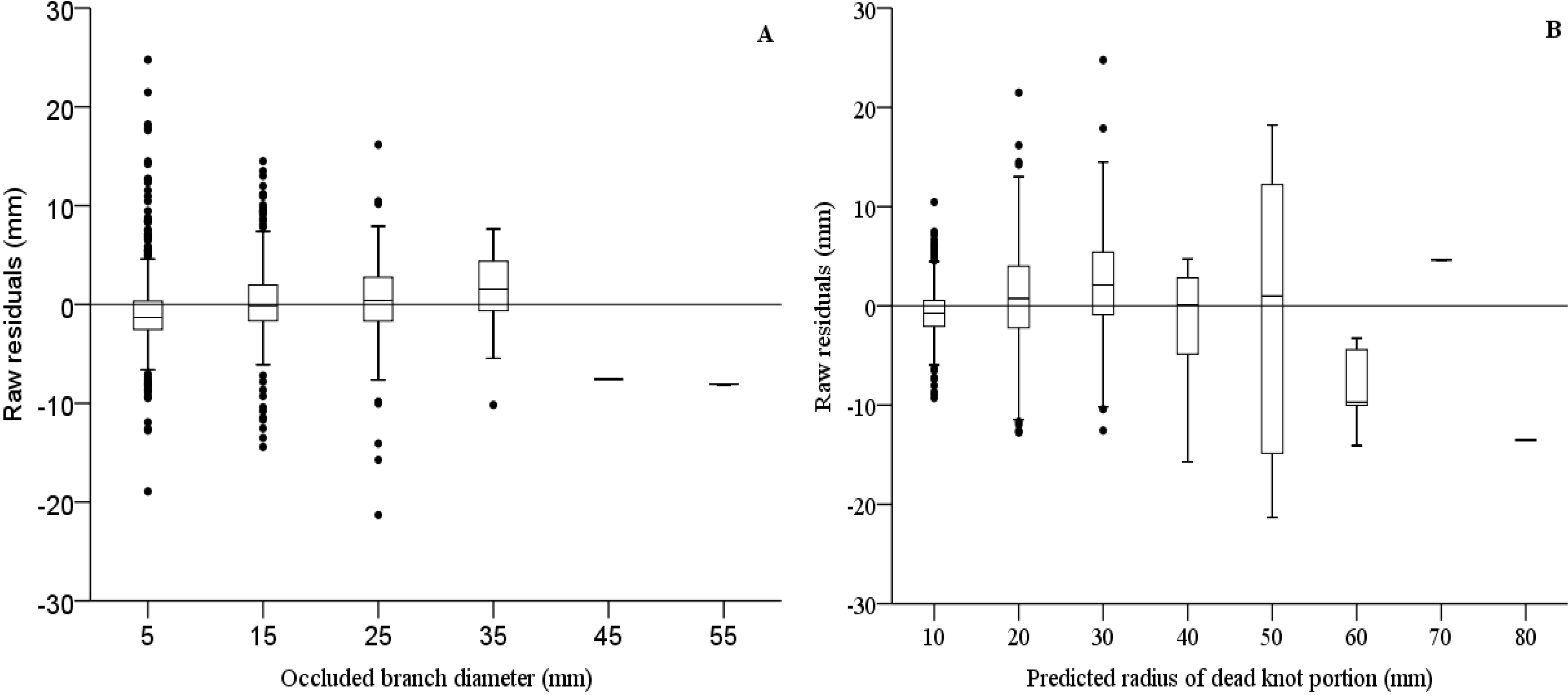
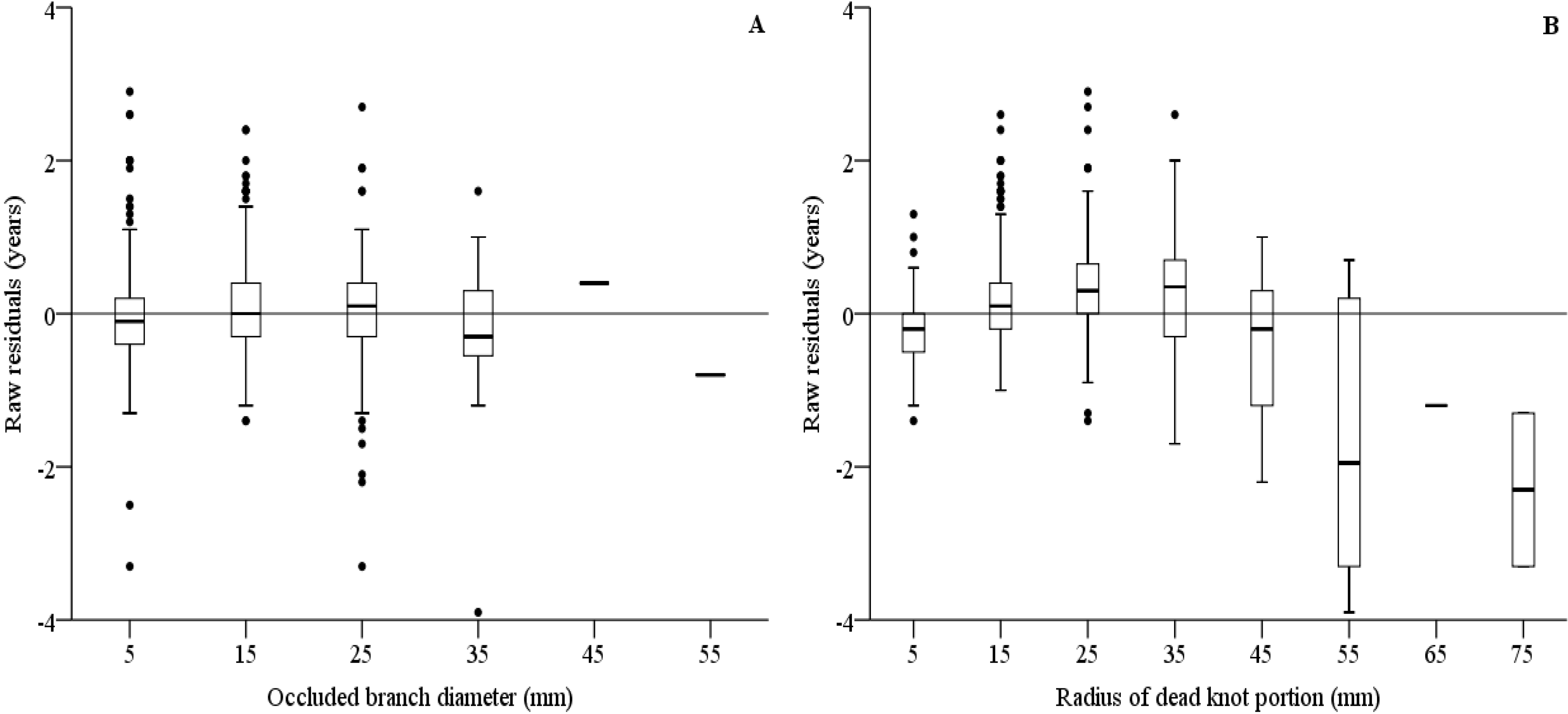
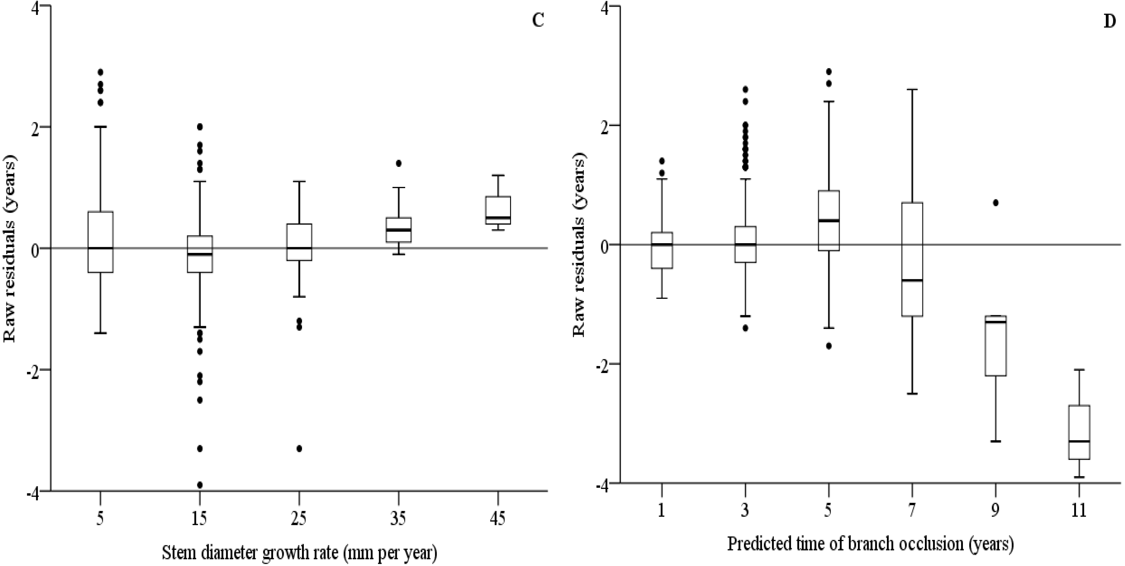
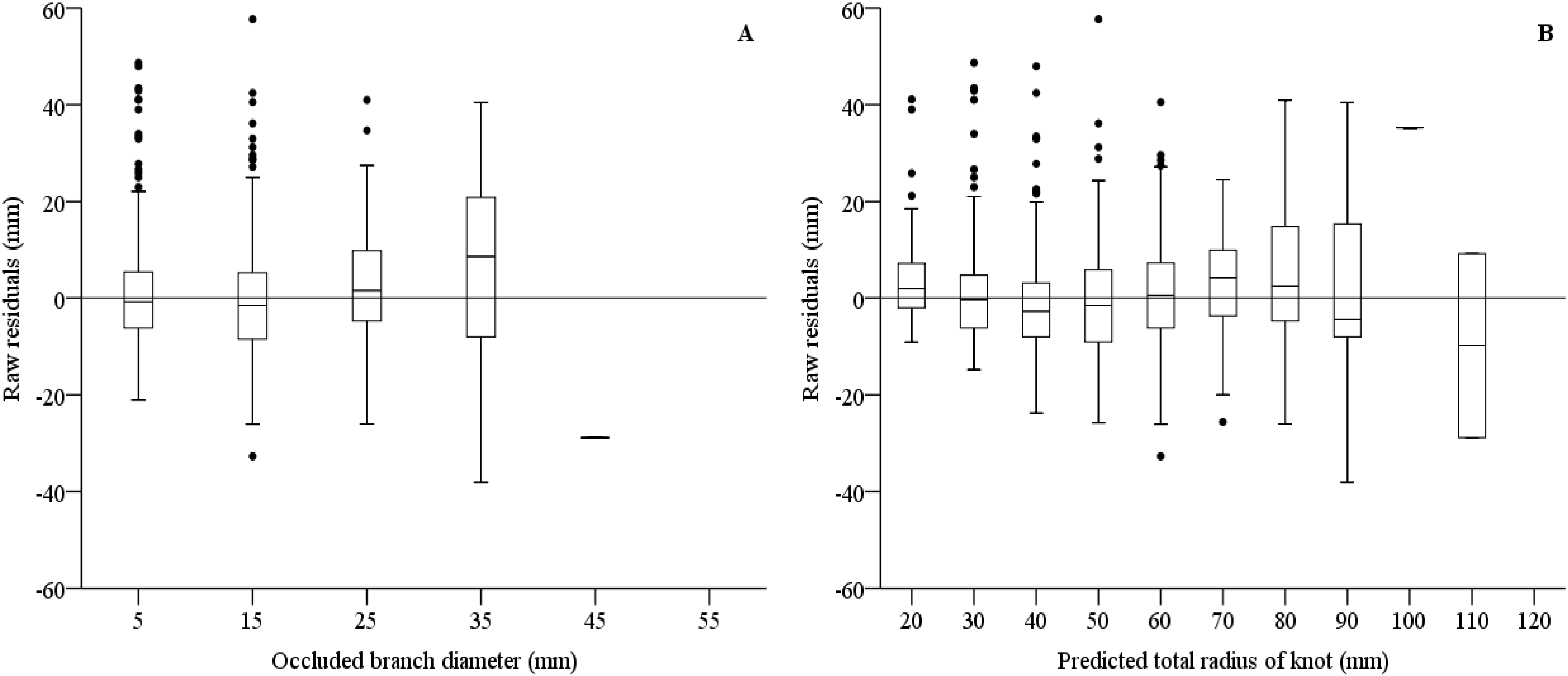
3.5. Models on Branch Occlusion and Knot Attributes
| Parameter | Estimate | Standard Error | T-value | Cl-Lower | Cl-Upper | Significance |
|---|---|---|---|---|---|---|
| Time of branch occlusion (Equation (1)) | ||||||
| Fixed parameters | ||||||
| a0 | 0.616 | 0.177 | 3.478 | 0.268 | 0.963 | <0.001 |
| a1 | 0.198 | 0.044 | 4.453 | 0.111 | 0.285 | <0.001 |
| a2 | 0.033 | 0.002 | 19.071 | 0.030 | 0.037 | <0.001 |
| a3 | −0.050 | 0.004 | −13.398 | −0.057 | −0.043 | <0.001 |
| Φ | 0.608 | |||||
| Error statistics | E = 0.0000 | |E| = 0.3623 | E² = 0.4996 | |||
| Radius of dead portion of knot (Equation (2)) | ||||||
| Fixed parameters | ||||||
| b0 | 2.010 | 0.139 | 14.474 | 1.738 | 2.282 | <0.001 |
| b1 | 0.535 | 0.032 | 16.530 | 0.472 | 0.599 | <0.001 |
| Random parameters | ||||||
| βptb | 53.110 | 2.071 | 25.644 | 49.202 | 57.328 | <0.001 |
| Error statistics | E = 0.0142 | |E| = 4.7864 | E² = 106.4202 | |||
| Total radius of knot (Equation (3)) | ||||||
| Fixed parameters | ||||||
| c0 | 2.003 | 0.081 | 24.765 | 1.844 | 2.162 | <0.001 |
| c1 | 0.678 | 0.017 | 40.059 | 0.645 | 0.711 | <0.001 |
| Random parameters | ||||||
| γptb | 122.748 | 4.787 | 25.643 | 113.715 | 132.498 | <0.001 |
| Error statistics | E = −0.0124 | |E| = 8.1513 | E² = 123.8880 | |||
| Insertion angle of the occluded branch (Equation (4)) | ||||||
| Fixed parameters | ||||||
| d0 | 4.151 | 0.031 | 134.398 | 4.090 | 4.211 | <0.001 |
| d1 | −0.047 | 0.010 | −4.776 | −0.066 | −0.028 | <0.001 |
| Random parameters | ||||||
| γptb | 77.414 | 3.018 | 25.652 | 71.720 | 83.561 | <0.001 |
| Error statistics | E = −0.01254 | |E| = 6.5097 | E² = 139.9267 | |||


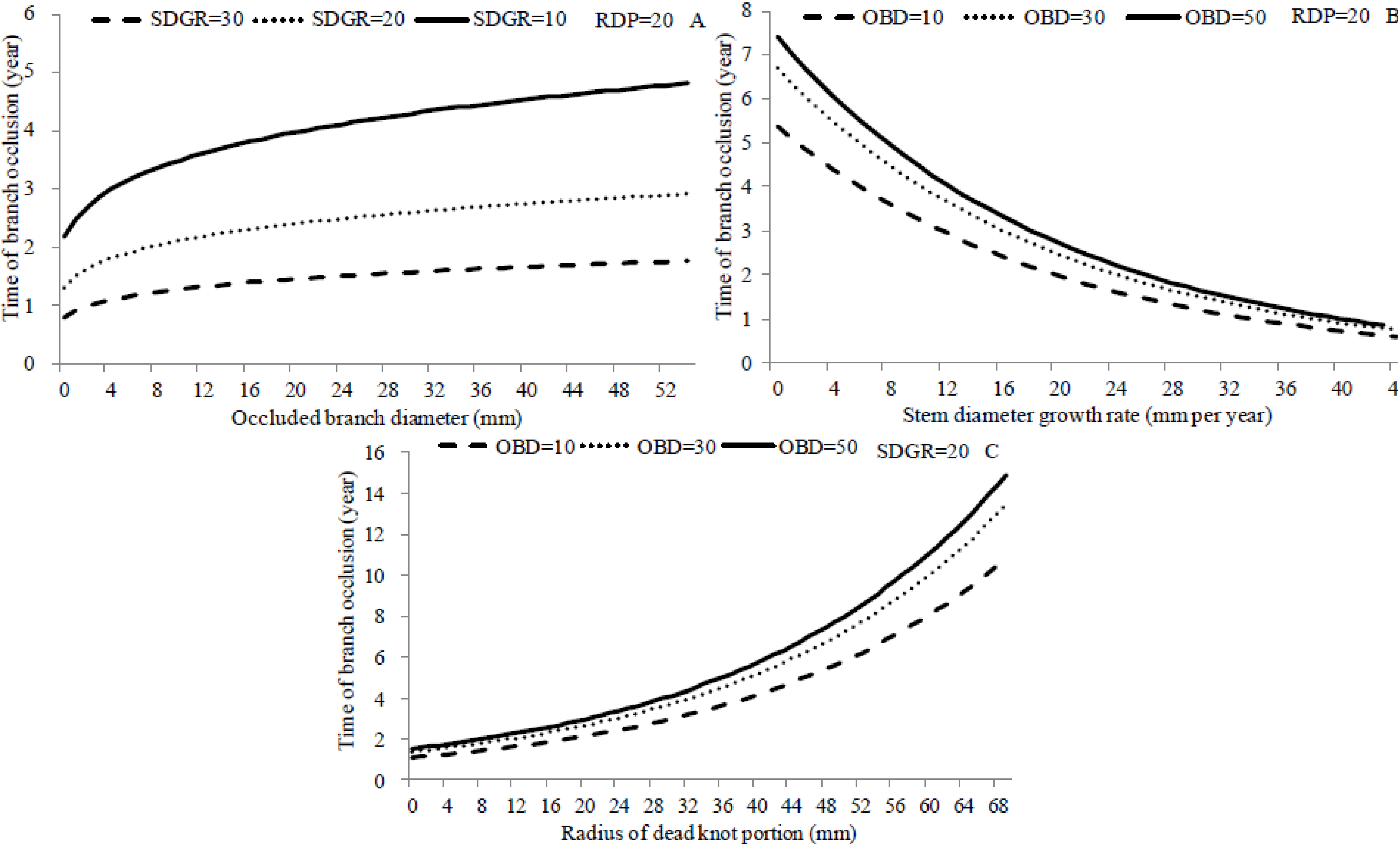
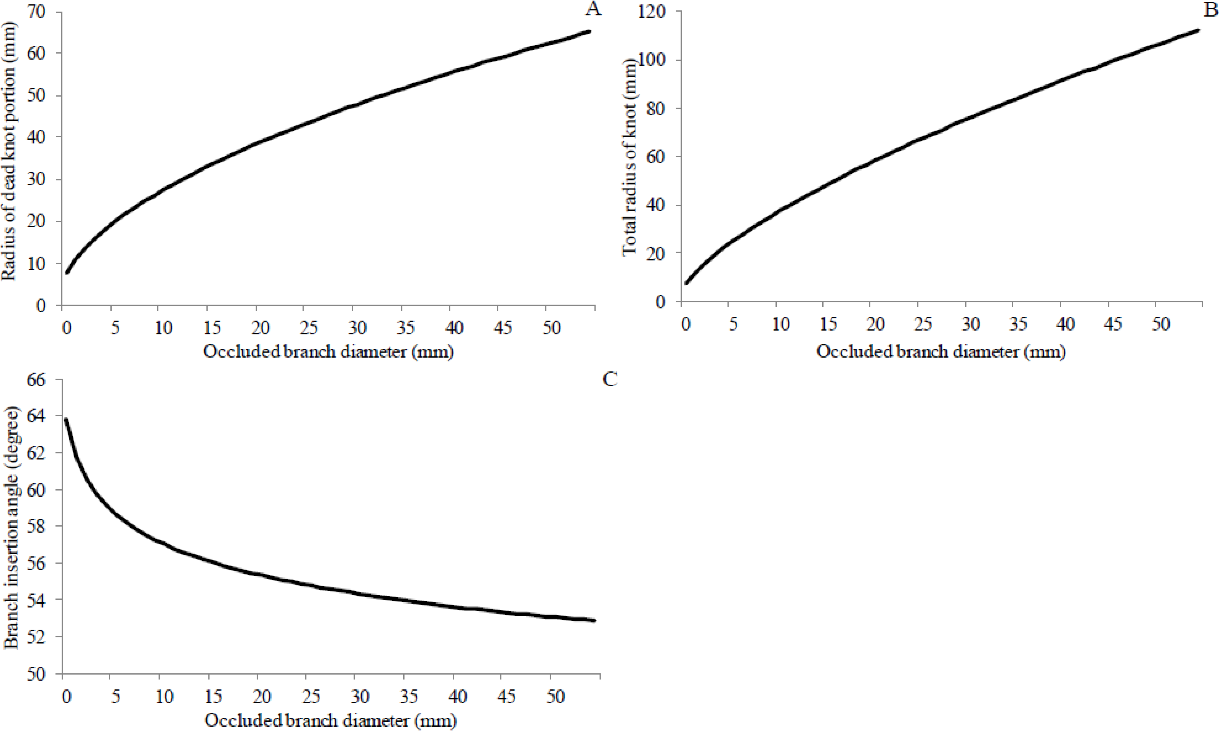
3.6. Simulations
4. Discussion
5. Conclusions
Acknowledgments
Author Contributions
Conflicts of Interest
References
- Sohngen, B.; Mendelsohn, R.; Sedjo, R. A global model of climate change impacts on timber markets. J. Agr. Resour. Econ. 2001, 26, 326–343. [Google Scholar]
- Mäkinen, H. Effect of stand density on the branch development of silver birch (Betula pendula Roth) in central Finland. Trees Struct. Funct. 2002, 16, 346–353. [Google Scholar]
- Alcorn, P.J.; Bauhus, J.; Thomas, D.S.; James, R.N.; Smith, R.G.B.; Nicotra, A.B. Photosynthetic response to green crown pruning in young plantation-grown Eucalyptus pilularis and E. cloeziana. For. Ecol. Manag. 2008, 255, 3827–3838. [Google Scholar] [CrossRef]
- Lowell, E.C.; Maguire, D.A.; Briggs, D.G.; Turnblom, E.C.; Jayawickrama, K.J.; Bryce, J. Effects of silviculture and genetics on branch/knot attributes of coastal pacific northwest douglas-fir and implications for wood quality—A Synthesis. Forests 2014, 5, 1717–1736. [Google Scholar] [CrossRef]
- O’Hara, K.L. Pruning wounds and occlusion: A long-standing conundrum in forestry. J. For. 2007, 105, 131–138. [Google Scholar]
- Johansson, K. Effects of initial spacing on the stem and branch properties and graded quality of Picea abies (L.) Karst. Scand. J. For. Res. 1992, 7, 503–514. [Google Scholar]
- Kellomäki, S.; Lämsä, P.; Oker-Blom, P.; Uusvaara, O. Management of Scots pine for high quality timber. Silva Carelica 1992, 23, 133. [Google Scholar]
- Deleuze, C.; Herve, J.C.; Colin, F.; Ribeyrolles, L. Modelling crown shape of Picea abies: Spacing effects. Can. J. For. Res. 1996, 26, 1957–1966. [Google Scholar] [CrossRef]
- Vestøl, G.I.; Høibø, O.A. Prediction of knot diameter in Picea abies (L.) Karst. Eur. J. Wood Prod. 2001, 59, 129–136. [Google Scholar] [CrossRef]
- Malimbwi, R.; Persson, A.; Iddi, S.; Chamshama, S.; Mwihomeke, S. Effects of spacing on yield and some wood properties of Pinus patula at Rongai, northern Tanzania. For. Ecol. Manag. 1992, 53, 297–306. [Google Scholar] [CrossRef]
- Kearney, D. Characterisation of Branching Patterns, Changes Caused by Variations in Initial Stocking and Implications for Silviculture, for E. grandis and E. pilularis Plantations in the North Coast Region of NSW. Bacheler Thesis, The Australian National University, Canberra, Australia, 1999. [Google Scholar]
- Pinkard, E.; Neilsen, W. Crown and stand characteristics of Eucalyptus nitens in response to initial spacing: Implications for thinning. For. Ecol. Manag. 2003, 172, 215–227. [Google Scholar] [CrossRef]
- Garber, S.M.; Maguire, D.A. Vertical trends in maximum branch diameter in two mixed-species spacing trials in the central Oregon Cascades. Can. J. For. Res. 2005, 35, 295–307. [Google Scholar] [CrossRef]
- Henskens, F.L.; Battaglia, M.; Cherry, M.L.; Beadle, C.L. Physiological basis of spacing effects on tree growth and form in Eucalyptus globulus. Trees Struct. Funct. 2001, 15, 365–377. [Google Scholar] [CrossRef]
- Alcorn, P.J.; Pyttel, P.; Bauhus, J.; Smith, R.G.B.; Thomas, D.; James, R.; Nicotra, A. Effects of initial planting density on branch development in 4-year-old plantation grown Eucalyptus pilularis and Eucalyptus cloeziana trees. For. Ecol. Manag. 2007, 252, 41–51. [Google Scholar] [CrossRef]
- Neilsen, W.A.; Gerrand, A.M. Growth and branching habit of Eucalyptus nitens at different spacing and the effect on final crop selection. For. Ecol. Manag. 1999, 123, 217–229. [Google Scholar] [CrossRef]
- Smith, R.G.B.; Dingle, J.; Kearney, D.; Monatgu, K. Branch occlusion after pruning in four contrasting sub-tropical Eucalypt species. J. Trop. For. Sci. 2006, 18, 117–123. [Google Scholar]
- Hein, S.; Spiecker, H. Comparative analysis of occluded branch characteristics for Fraxinus excelsior and Acer pseudoplatanus with natural and artifical pruning. Can. J. For. Res. 2007, 37, 1414–1426. [Google Scholar] [CrossRef]
- Hein, S. Knot attributes and occlusion of naturally pruned branches of Fagus sylvatica. For. Ecol. Manag. 2008, 256, 2046–2057. [Google Scholar] [CrossRef]
- O’Hara, K.L.; Buckland, P.A. Prediction of pruning wound occlusion and defect core size in ponderosa pine. West. J. Appl. For. 1996, 11, 40–43. [Google Scholar]
- Petruncio, M.; Briggs, D.; Barbour, R.J. Predicting pruned branch stub occlusion in young, coastal Douglas-fir. Can. J. For. Res. 1997, 27, 1074–1082. [Google Scholar] [CrossRef]
- Trincado, G.; Burkhart, H.E. A model of knot shape and volume in Loblolly pine trees. Wood Fiber Sci. 2008, 40, 634–646. [Google Scholar]
- Grah, R.F. Relationship between tree spacing, knot size, and log quality in young Douglas-fir stands. J. For. 1961, 59, 270–272. [Google Scholar]
- Moberg, L. Variation in knot size of Pinus sylvestris in two initial spacing trials. Silva Fennica 1999, 33, 131–144. [Google Scholar] [CrossRef]
- Vestøl, G.I.; Colin, F.; Loubère, M. Influence of progeny and initial stand density on the relationship between diameter at breast height and knot diameter of Picea abies. Scand. J. For. Res. 1999, 14, 470–480. [Google Scholar]
- Zeng, J.; Wang, Z.; Zhou, S.; Bai, J.; Zheng, H. Allozyme variation and population genetic structure of Betula alnoides from Guangxi, China. Biochem. Genet. 2003, 41, 61–75. [Google Scholar] [CrossRef] [PubMed]
- Zeng, J.; Guo, W.; Zhao, Z.; Qijie, W.; Yin, G.; Zheng, H. Domestication of Betula alnoides in China: Current Status and Perspectives. For. Res. 2005, 12, 379–384. [Google Scholar]
- Zeng, J.; Zheng, H.; Weng, Q. Geographic distributions and ecological conditions of Betula alnoides in China. For. Res. 1999, 12, 479–484. [Google Scholar]
- McCullagh, P.; Nelder, J.A. Generalized Linear Models; Chapman and Hall: London, UK, 1989; p. 511. [Google Scholar]
- Dănescu, A.; Ehring, A.; Bauhus, J.; Albrecht, A.; Hein, S. Modelling discoloration and duration of branch occlusion following green pruning in Acer pseudoplatanus and Fraxinus excelsior. For. Ecol. Manag. 2015, 335, 87–98. [Google Scholar] [CrossRef]
- Ilstedt, B.; Eriksson, G. Quality of intra- and interprovenance families of Picea abies (L.) Karst. Scand. J. For. Res. 1986, 1, 153–166. [Google Scholar]
- Clair, J.B.S. Genetic variation in tree structure and its relation to size in Douglas-fir. II. Crown form, branch characters, and foliage characters. Can. J. For. Res. 1994, 24, 1236–1247. [Google Scholar] [CrossRef]
- Maguire, D.; Moeur, M.; Bennett, W. Models for describing basal diameter and vertical distribution of primary branches in young Douglas-fir. For. Ecol. Manag. 1994, 63, 23–55. [Google Scholar] [CrossRef]
- Weiskittel, A.R.; Maguire, D.A.; Monserud, R.A. Modeling crown structural responses to competing vegetation control, thinning, fertilization, and Swiss needle cast in coastal Douglas-fir of the Pacific Northwest, USA. For. Ecol. Manag. 2007, 245, 96–109. [Google Scholar] [CrossRef]
- Briggs, D.; Ingaramo, L.; Turnblom, E. Number and diameter of breast-height region branches in a Douglas-fir spacing trial and linkage to log quality. For. Prod. J. 2007, 57, 28. [Google Scholar]
- Newton, M.; Lachenbruch, B.; Robbins, J.M.; Cole, E.C. Branch diameter and longevity linked to plantation spacing and rectangularity in young Douglas-fir. For. Ecol. Manag. 2012, 266, 75–82. [Google Scholar] [CrossRef]
- Glencross, K.; Nichols, J.D.; Grant, J.; Sethy, M.; Smith, R.G.B. Spacing affects stem form, early growth and branching in young whitewood (Endospermum medullosum) plantations in Vanuatu. Int. Forest. Rev. 2012, 14, 442–451. [Google Scholar] [CrossRef]
- Kearney, D.; James, R.; Montagu, K.; Smith, R.G.B. The effect of initial planting density on branching characteristics of Eucalyptus pilularis and E. grandis. Aust. For. 2007, 70, 264–268. [Google Scholar] [CrossRef]
- Kellomäki, S.; Oker-Blom, P. Canopy structure and light climate in a young Scots pine stand. Silva Fenn. 1983, 17, 1–21. [Google Scholar] [CrossRef]
- Niemistö, P. Influence of initial spacing and row-to-row distance on the crown and branch properties and taper of silver birch (Betula pendula). Scand. J. For. Res. 1995, 10, 235–244. [Google Scholar] [CrossRef]
- Mäkinen, H. Effect of stand density on radial growth of branches of Scots pine in southern and central Finland. Can. J. For. Res. 1999, 29, 1216–1224. [Google Scholar] [CrossRef]
© 2015 by the authors; licensee MDPI, Basel, Switzerland. This article is an open access article distributed under the terms and conditions of the Creative Commons Attribution license (http://creativecommons.org/licenses/by/4.0/).
Share and Cite
Wang, C.; Zhao, Z.; Hein, S.; Zeng, J.; Schuler, J.; Guo, J.; Guo, W.; Zeng, J. Effect of Planting Density on Knot Attributes and Branch Occlusion of Betula alnoides under Natural Pruning in Southern China. Forests 2015, 6, 1343-1361. https://doi.org/10.3390/f6041343
Wang C, Zhao Z, Hein S, Zeng J, Schuler J, Guo J, Guo W, Zeng J. Effect of Planting Density on Knot Attributes and Branch Occlusion of Betula alnoides under Natural Pruning in Southern China. Forests. 2015; 6(4):1343-1361. https://doi.org/10.3390/f6041343
Chicago/Turabian StyleWang, Chunsheng, Zhigang Zhao, Sebastian Hein, Ji Zeng, Johanna Schuler, Junjie Guo, Wenfu Guo, and Jie Zeng. 2015. "Effect of Planting Density on Knot Attributes and Branch Occlusion of Betula alnoides under Natural Pruning in Southern China" Forests 6, no. 4: 1343-1361. https://doi.org/10.3390/f6041343
APA StyleWang, C., Zhao, Z., Hein, S., Zeng, J., Schuler, J., Guo, J., Guo, W., & Zeng, J. (2015). Effect of Planting Density on Knot Attributes and Branch Occlusion of Betula alnoides under Natural Pruning in Southern China. Forests, 6(4), 1343-1361. https://doi.org/10.3390/f6041343