1. Introduction
The search for an objective definition of forest health and a framework for its assessment have been elusive [
1]. Several definitions of forest health have been proposed that range from utilitarian to ecological in perspective [
2]. Recently, Teale and Castello [
3] proposed a two-part definition of forest health. The first is maintenance of a sustainable size class structure, within the ecological parameters of the species, at the landscape level as defined by Manion and Griffin [
4]. The second involves meeting the management objectives for the specific forest. Sustainability, however, occupies a pivotal role because long-term management objectives become unattainable if the forest is unsustainable. Recent definitions of forest health incorporate important ecological qualities such as ecosystem balance, resilience to disturbance, plant and animal community function, sustainable productivity, as well as national, political, social, or spiritual concerns [
1,
5]. These factors are included in the management objective component of our definition of forest health. This study focuses on the sustainability aspect of the assessment of a healthy forest.
How does one define forest sustainability? Like forest health, sustainability has been difficult to define and to measure because people have differing and often competing priorities that reflect their values at a particular point in time and often come at the expense of others. For example, stakeholders (e.g., landowners, government agencies and forest ecologists) often disagree on what specific resources should be sustained and how forests should be managed. Furthermore, forest ecosystems are complex and develop slowly, confounding measures of sustainability [
6]. The more traditional ecological concept of forest sustainability is based on the maintenance of forest ecosystem composition, structure, and function over the long term [
2,
7]. These approaches embody what many intuitively envision as a healthy forest, but are subjective, difficult to assess or both. Manion and Griffin [
4] and Didion
et al. [
8] reasoned that stand age class structure be used to compare the combined effects of human and natural disturbances at the landscape scale over long time periods to assess the long-term sustainability of a forest. Didion
et al. [
8] utilized a simulation model-sensitivity analysis of forest age structure to evaluate the impacts of management regimes and fire on boreal forest sustainability. In principle, this approach is consistent with the diameter class structure approach of Manion and Griffin [
4] and Zhang
et al. [
9] who used diameter as a surrogate for age [
10].
We support an uncomplicated definition of forest sustainability simply as structural stability, and fully recognize that forests are dynamic, not static ecosystems as our definition may infer. We do not imply that forest structure or composition must remain unchanged for that forest to be considered sustainable or indeed, healthy. Rather it is the equivalence of baseline and observed mortality that must remain stable for the forest to be considered structurally sustainable. This approach gives us a frame of reference within which to evaluate changes in structure. It gives us the ability to objectively determine the scope and direction of change in structure and composition, which provides the ecological framework for objective management decisions. It sets the stage for the quantification of forest stability or change that hinges on a comparison of the current, observed mortality with a context-specific, theoretical value termed baseline mortality. The calculation of current baseline mortality values are independent of prior BM values. Therefore, it is irrelevant whether forests are managed or not because the approach we developed applies to both systems.
The comparison of baseline to observed mortality is possible due to the q-ratio or its special case known as the Law of de Liocourt that describes the size structure of a forest (density of stems) as a function of stem diameter [
11,
12]. The q ratio applies only to uneven-aged stands; but since this is a landscape-level analytical approach, a forest consisting of a mosaic of even-aged stands can be uneven-aged at this scale [
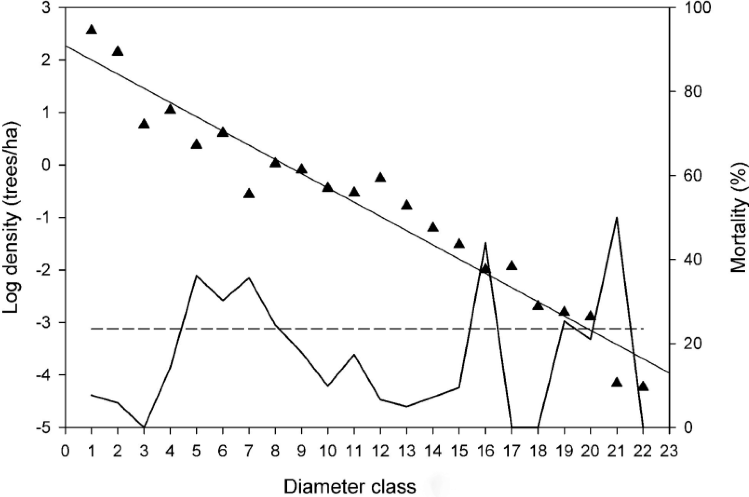
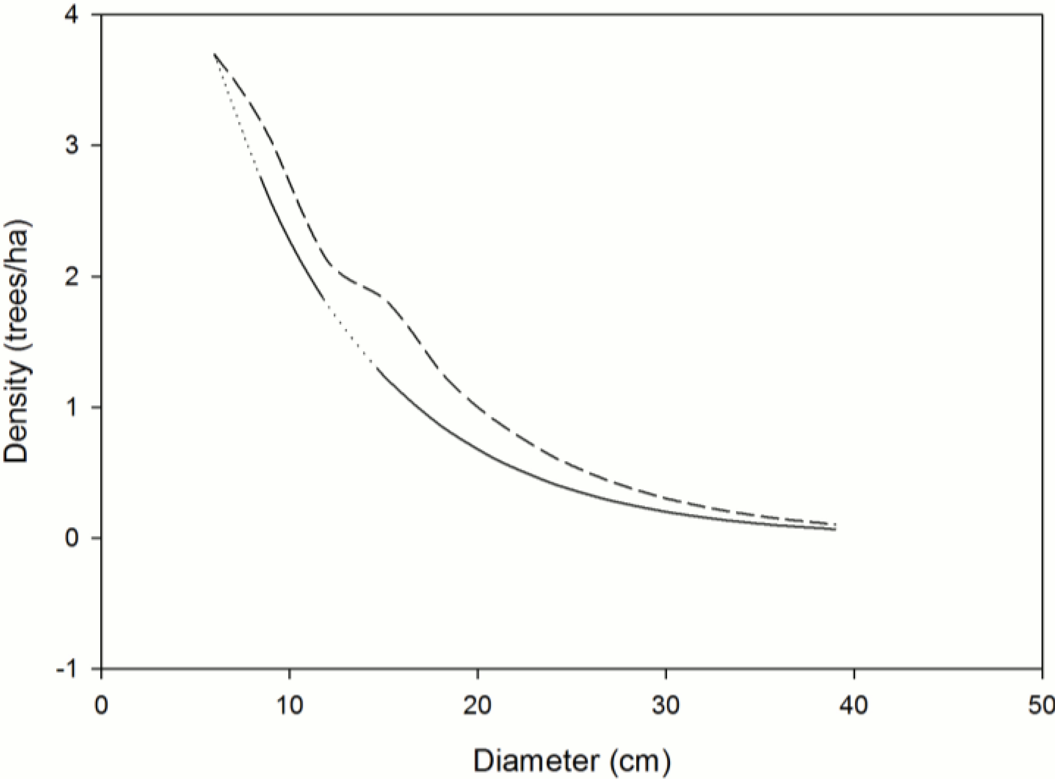
10]. Commonly, but not always, this relationship is described by the negative exponential function. When the diameter distribution closely fits the negative exponential function, the slope of the line is inversely proportional to the number of trees that must be removed from the population as the surviving trees in each diameter class grow into the next larger diameter class—for the size structure of the forest to remain stable. The baseline mortality is derived from this slope, and for diameter distributions that fit the negative exponential function, it is constant across all diameter classes (
Figure 1). The method we describe potentially can be modified accordingly in instances where other probability density functions more closely approximate diameter distributions [
9].
Figure 1.
Log-linear plot of a hypothetical diameter distribution (▲), the baseline mortality calculated from the log-linear plot (- - -), and hypothetical currently observed mortality by diameter class (solid line without triangles).
Figure 1.
Log-linear plot of a hypothetical diameter distribution (▲), the baseline mortality calculated from the log-linear plot (- - -), and hypothetical currently observed mortality by diameter class (solid line without triangles).
Baseline mortality is the percent of trees in each diameter class that will normally die in a structurally sustainable forest in the time it takes for the trees to grow into the next larger diameter class. The width of the diameter classes, therefore, must correspond to the time frame in which the observed mortality occurred in order to provide a basis for the evaluation of mortality from all causes. For example, if dead stems are identifiable and measureable for a maximum of 20 years, then the diameter class width (DC bin size) in a baseline mortality analysis must represent 20 years of growth. The subjects of this paper are the precise relationship between observed and baseline mortality and how much observed mortality must deviate from the baseline before we can expect a change in the size structure of the forest.
Here, we use available forest inventory datasets to assess the structural sustainability of 22 tree species in disparate geographic regions using the baseline mortality approach. We hypothesize that the structural sustainability of forest tree species populations and the impacts of known and unknown disturbances on their sustainability can be objectively and quantitatively assessed. Our objectives were to develop a quantitative index using a statistical approach to objectively distinguish between sustainable and unsustainable diameter distributions for 22 species and populations, and to evaluate the impacts of known disturbances on four of them. We used logistic regression to provide an unbiased threshold estimate. All sustainability scores above and below this estimate were deemed unsustainable and sustainable, respectively. We also developed a computer software package that performs all of the calculations necessary to conduct these analyses, and it is available on the SUNY-ESF website.
3. Results and Discussion
All of the species that we evaluated showed negative exponential diameter distributions with model
R2 > 0.82. Therefore, baseline mortality (BM%) was constant across all diameter classes for each of the 22 species (
Table 2).
Table 2.
Baseline percent mortality, correlation coefficient of regression of natural log of diameter distribution fit to the negative exponential model, diameter distribution metrics, discriminant function score, and cluster category for each of the 22 species populations.
Table 2.
Baseline percent mortality, correlation coefficient of regression of natural log of diameter distribution fit to the negative exponential model, diameter distribution metrics, discriminant function score, and cluster category for each of the 22 species populations.
| Species | BM (%) 1 | R 2 | MAG 3 | AGG 4 | DM 5 | CHG 6 | RA 7 | DF Score 8 | Cluster 9 |
|---|
| A. amabilis | 18.1 | 0.98 | 4.7 | 0 | 5 | 0.70 | 0.036 | 4.3 | S |
| T. plicata | 11.3 | 0.86 | 19.4 | 1 | 5 | 0.70 | 0.071 | 12.9 | S |
| T. brevifolia | 30.2 | 0.88 | 29 | 0 | 5 | 0.52 | 0.167 | 17.6 | S |
| A. magnifica | 11.3 | 0.89 | 31.3 | 1 | 5 | 0.61 | 0.075 | 19.4 | S |
| T. heterophylla | 18.1 | 0.96 | 38.9 | 2 | 12 | 0.61 | 0.179 | 27.2 | S |
| P. glauca | 31.6 | 0.96 | 46.0 | 1 | 5 | 0.34 | 0.222 | 27.6 | S |
| A. concolor | 13.9 | 0.92 | 65.8 | 2 | 7 | 0.67 | 0.172 | 39.6 | S |
| A. lasiocarpa | 23.7 | 0.82 | 91.6 | 2 | 5 | 0.44 | 0.357 | 52.9 | S |
| A. saccharum | 20.5 | 0.96 | 89.1 | 2 | 9 | 0.69 | 0.267 | 53.0 | S |
| B. alleghaniensis | 18.1 | 0.95 | 89.9 | 2 | 12 | 0.58 | 0.226 | 54.7 | S |
| T. canadensis | 20.5 | 0.95 | 98.1 | 2 | 5 | 0.54 | 0.31 | 56.3 | S |
| P. strobus * | 13.9 | 0.82 | 144.4 | 2 | 12 | 0.63 | 0.296 | 84.1 | S |
| P. engelmannii * | 21.3 | 0.91 | 107.3 | 3 | 9 | 0.38 | 0.375 | 63.8 | U, + |
| P. rubens * | 25.9 | 0.95 | 110.5 | 3 | 9 | 0.48 | 0.333 | 65.4 | U, − |
| N. solandri | 33.0 | 0.86 | 144.7 | 3 | 12 | 0.48 | 0.54 | 85.2 | U, − |
| C. decurrens | 13.9 | 0.89 | 175.7 | 5 | 14 | 0.30 | 0.351 | 104.2 | U, − |
| P. serotina | 21.3 | 0.92 | 192.2 | 5 | 12 | 0.37 | 0.56 | 112.3 | U, +, − |
| A. balsamea | 40.5 | 0.98 | 228.1 | 4 | 9 | 0.42 | 0.60 | 129.7 | U, − |
| A. rubrum | 26.7 | 0.95 | 224.5 | 6 | 12 | 0.28 | 0.64 | 130.5 | U, − |
| P. ponderosa | 38.1 | 0.96 | 246.7 | 4 | 14 | 0.19 | 0.56 | 141.9 | U, − |
| F. grandifolia | 30.2 | 0.96 | 334.9 | 6 | 12 | 0.39 | 0.71 | 190.0 | U, +, − |
| P. lambertiana | 14.8 | 0.82 | 438.0 | 7 | 14 | 0.28 | 0.72 | 247.2 | U, + |
Cluster analysis using the five mortality metrics classified the 22 species populations into two clusters. The discriminant analysis on the two clusters yielded one significant canonical root (Wilk’s lambda = 0.2194;
F (5,16) = 11.38;
p < 0.0001], confirming the two clusters were statistically distinguishable. Moreover, all five metrics were significantly (
p < 0.05) important for cluster separation. The following discriminant function based on the 1000 bootstrapped discriminant analyses was derived from the mean pooled within-class canonical coefficients:
then, the score of the
DF function (Equation 8) was computed for each species (
Table 2).
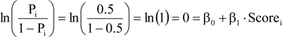
We view the bootstrapped discriminant function as a “structural sustainability index” because the five metrics were based on patterns of observed mortality and existing diameter distributions, and were designed to compare mortality among different populations of trees, and to reflect potential future changes in the size structures of the species populations. For the sustainable group, the lowest sustainable score was 4.27 and the highest score was 56.3 (mean = 33.2 and median = 27.6). For the unsustainable group, the lowest unsustainable score was 85.2 and the highest score was 247.2 (mean = 142.6 and median = 130.1). The threshold score (Equation 7), defined as the sustainability score with an equal chance of being designated sustainable or unsustainable, was derived from logistic regression model parameters in Equation (4) (i.e., β0/−β1 = −7.1002/0.1006 = 70.58) Thus, species with scores less than 70.58 were sustainable and those with scores over this threshold were unsustainable.
Discriminant analysis had an apparent total error rate of 0.14 (0.08 for sustainable group and 0.20 for unsustainable group).
P. engelmannii and
P. rubens were misclassified as sustainable, and
P. strobus was misclassified as unsustainable (
Table 2).
Sustainability problems were evident in each temperate forest type, and in each of the three old-growth western coniferous forest regions (PNW, IM, and SN), although most of the unsustainable species were located in the Adirondack Forest Preserve of New York (
Table 1 and
Table 2). The results of individual baseline mortality analyses, however, apply only to the species in the forests that were assessed, and should not be extrapolated to represent the sustainability of that species in other forested regions.
In total, 12 of the 22 species populations were categorized as structurally sustainable and 10 as unsustainable (
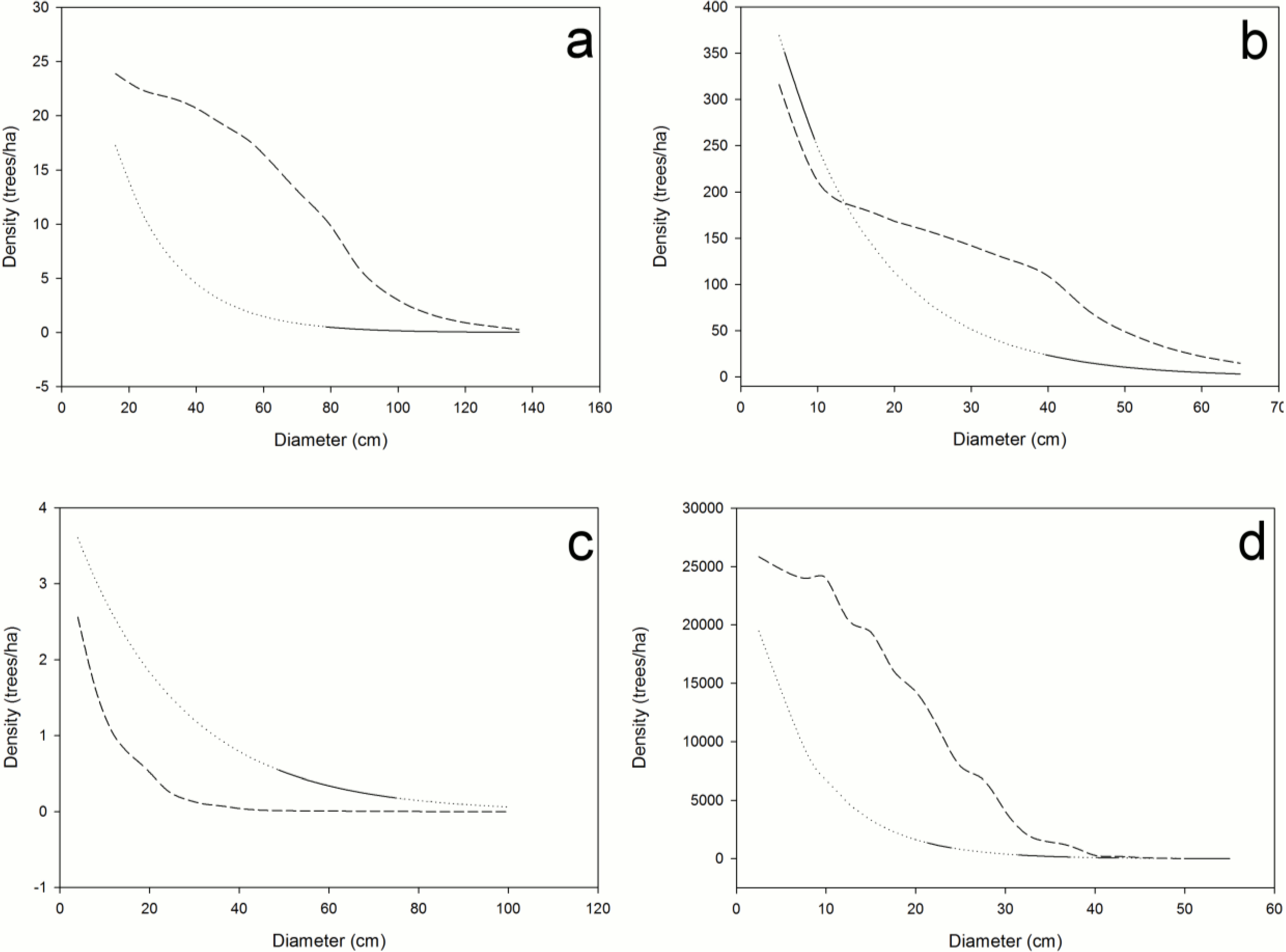
Table 2). Significant deviations between observed and baseline mortality in some DCs does not necessarily threaten the structural sustainability of a species. For example, the sustainable diameter distribution of
T. brevifolia (PNW,
Figure 2) illustrates overall congruence of the projected and control diameter distributions even though significant differences between observed and expected dead occur in some diameter classes.
Figure 2.
Calculated distributions illustrating the impact of currently observed mortality on sustainability of Taxus brevifolia (PNW); congruence of control (—) and projected (- - -) size class structures indicates that the observed mortalities will not significantly impact forest structure; diameter classes with significant differences between observed and baseline mortality are shown as dotted lines; dashed line segments above or below the solid/dotted line indicate insufficient or excessive mortality, respectively; future diameter distributions hold ingrowth, recruitment, and mortality constant.
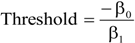
Structural unsustainability can be caused by either excessive or insufficient mortality (
Figure 3a–d). Indeed, current mortality levels of ponderosa pine (
Figure 3a) in the sampled old-growth stands in the PNW and IM regions are insufficient (
i.e., observed significantly less than expected dead) to maintain their structural stability. The accumulation of
P. ponderosa is attributable to decades of fire suppression [
17,
18], which may explain the low mortality that we observed (
Figure 3a). High density stands of low vigor often result in outbreaks of mountain pine beetle (
Dendroctonus ponderosae, MPB) and catastrophic crown fires, which have occurred in pine stands in both Arizona and Oregon [
18,
19]. Thus, the baseline mortality method successfully identified this well-recognized problem in old-growth ponderosa pine forests of the western United States. One potential problem using this method in such high-severity, fire-prone ecosystems is that small trees might be completely consumed by fire that may not allow all dead trees across all diameter classes to remain identifiable. In such cases, a lower diameter limit could be identified for baseline mortality determination.
Figure 3.
Calculated distributions illustrating the impact of currently observed mortality on sustainability of (a) Pinus ponderosa (PNW + IM), (b) Nothofagus solandri (NZ), (c) Pinus lambertiana (SN), and (d) Fagus grandifolia (AFP); lack of congruence of control (—) and projected (- - -) size class structures indicates that the observed mortalities will significantly impact forest structure; diameter classes with significant differences between observed and expected dead trees are shown as dotted lines; dashed line segments above or below the solid/dotted line indicate insufficient or excessive mortality, respectively; future diameter distributions hold ingrowth, recruitment, and mortality constant.
Nothofagus solandri exists as a mosaic of even-aged stands on both the North and South Islands of New Zealand. Stand structure in these forests is influenced by large-scale disturbances, such as the snowstorms of 1968 and 1973, and the 1994 earthquake; which caused widespread landslides and subsequent tree damage and mortality on the South Island [
20]. The response to these events created an unsustainable structure consisting of too many trees (insufficient mortality) in the small to intermediate size classes (diameter classes 2–10 in
Figure 3b represent diameters of 10–40 cm, respectively) from the 1999 dataset we evaluated (
Table 2,
Figure 3b). Hurst
et al. [
21] observed annual mortality rates in these same stands to decrease from 0.022 in 1974–1983 to 0.019 in 1983–1993, and finally to 0.018 in 1993–2004; and that this decrease was not attributable to crowding effects over time. Our analysis confirms their conclusions, and suggests that future, excessive mortality is likely, and will be necessary to restore landscape-level sustainability to these forests.
Excessive mortality (
i.e., observed significantly greater than expected dead) also can cause structural sustainability problems (
Figure 3c,d). High levels of mortality across all diameter classes of
P. lambertiana in the SN region (
Figure 3c) is most likely attributable to white pine blister rust [
14]; a non-native, invasive fungal disease of five-needle pines in North America [
22] that could extirpate this species from these stands should it continue at these high levels. The baseline mortality method confirmed excessive levels of mortality, which we attribute to this devastating invasive pathogen.
In the northern hardwood forests of the AFP, our analyses identify five structurally unsustainable species populations including
A. balsamea, A. rubrum, F. grandifolia, Picea rubens, and
P. serotina (
Table 2). The unsustainability of American beech is attributable to the invasive disease complex known as beech bark disease, which explains the insufficient mortality in the small DCs and excessive mortality in the larger DCs (
Figure 3d) [
23]. Beech bark disease induced-mortality of large, mature trees results in dense thickets of young beech of root-sprout origin. The current and projected structures are undesirable from a management perspective because the excess of small stems and death of larger trees are significant management challenges. Nonetheless, knowing the current size structure and how it is changing provides an opportunity to develop proactive management strategies for beech. Although unknown, we suspect that the cause of unsustainability of
P. serotina may be attributable to past cutting practices in this region. The insufficient mortality observed in
A. balsamea and
P. rubens may be a natural response to a regionwide windstorm in 1995 that caused severe blowdown. Similarly, insufficient mortality observed in the
A. rubrum population may be the result of a systematic successional shift in the abundance of this species that is occurring in many areas. All structural changes must be interpreted in the light of the ecological characteristics of the species, disturbance history, and whether or not the changing structure interferes with the management objectives for the forest. Periodic BM analyses for these species could reveal whether the structural unsustainability was temporary or becomes a forest health issue.
Increasing rates of mortality detected in the sampled old-growth coniferous forest stands of the western U.S. was attributed to climate change by van Mantgem
et al. [
14]. However, their study utilized pooled species data so extrapolation of their conclusions to our individual species analyses should be made with caution. Nevertheless, the baseline mortality method suggests that the increasing mortality they observed is excessive for
P. lambertiana, the cause of which is white pine blister rust; and
P. engelmannii for which the cause is unknown. The other old-growth stands of western conifer species that were structurally unsustainable are
C. decurrens in the SN region, and
P. ponderosa in the PNW and IM regions, which are both attributable to insufficient mortality.
Structural stability (
i.e., sustainability, assessed this way) has several advantages over other methods. First, dead trees are comparatively easy to recognize and to count, whereas the ecological processes that regulate a forest ecosystem (e.g., energy and nutrient flow, trophic-level interactions, ecosystem balance, and resilience) are not. Second, forest health monitoring programs typically focus on tree crown condition over time to gauge the health of a forest [
24]. However, crown condition is reversible, and its measurement subjective. More importantly, reliance on crown health confuses individual tree health (organism level) with forest health (population to landscape level). Third, the baseline mortality approach provides a framework within which to detect elevated (or insufficient) levels of mortality. Structurally sustainable, healthy forests have dead and dying trees, but now we can determine if that mortality is too much or too little. Fourth, routinely collected forest inventory data (species, growth rates, number and size of living and dead trees) are sufficient to conduct these analyses. Lastly, baseline mortality and its relationship to observed mortality can provide a forward-looking, prospective approach to the assessment of structural sustainability. Tree mortality data are collected annually by the USDA Forest Service [
25] and agencies in other countries and trends in mortality often are evaluated retrospectively by comparing current to historical mortality levels. This approach assumes that historical mortality levels are an appropriate frame of reference, which may not be true. Baseline mortality provides a more rational baseline to which currently observed mortality can be compared, and has the added advantage of being able to prospectively assess the impacts of current mortality levels on future forest structure and composition.
The multivariate structural sustainability index and threshold value are empirically derived from 21 temperate and one boreal forest tree species. It may eventually be possible to develop a global sustainability index once more forest species from the temperate, boreal, tropical and subtropical forests of the world are evaluated. At that time it may be possible to compare the impact of global disturbances (e.g., climate change) on forest structural sustainability both spatially and temporally. Until then, we propose that a regionally derived structural sustainability index score be included as one more additional and important consideration when forestland managers or landowners assess the sustainability/health of their forests.
Although the baseline mortality concept and associated index may not be appropriate for certain species (e.g., those with diameter distributions other than negative exponential), the ramifications of our proposed methods are significant. A standardized analysis that permits the objective and quantitative assessment of the structural sustainability of a forest provides the ability to determine the impact of natural and anthropogenic disturbance agents, including management activity, on that forest. We have used the method to verify the impacts of known disturbance agents on four species, and the results support our hypothesis that the method can identify or elucidate structurally unsustainable forests. Plus, it provides the ability to recognize a potential sustainability problem before the cause is known,
e.g.,
A. balsamea, A. rubrum, C. decurrens, Picea engelmannii, P. rubens, and
P. serotina (
Table 2); and to alert forest health professionals and agencies to the potential need for action. This approach may enable comparison of the impacts of disturbances in time and space on forests on a global scale. Government agencies, NGOs and forest health professionals also can prioritize resource allocation and research needs based upon an objective assessment of how native and invasive pests and pathogens as well as other disturbances affect structural sustainability. Sturrock
et al. [
26] call for a triage system to help ecologists and forest managers decide which forest types or species are most threatened by climate change or other disturbances and to develop long-term management plans. Finally, distinguishing between stands with different structural conditions is an essential feature of all useful structural indices that can reveal clues to the ecological processes that drive structure [
27]. Methods that can differentially distinguish stands with changing structures are needed [
27]. The baseline mortality approach answers these calls, and promotes the objective assessment of forest structural sustainability in a manner that is unique in its clarity and globally applicable.
A software package is available at the following URL [
28] that performs all of the calculations for these analyses once all of the necessary data (dbh and health status (living or dead) of all trees of the species of interest in the area, and DC bin size) are input.


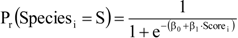
 is expressed as a linear function of the “Score”: