We first give an overview on the Group I results, as the algorithm was developed and adjusted utilizing these branches. Afterwards, a deeper analysis of the Group II results is presented, including a comparison to ground truth measurements, as well as an examination between the input point cloud and the resulting cylinder model. An analysis of the artificial point cloud results, where all structure parameters are known a priori, is performed. Two allometric models derived from 24 Group III trees will conclude the results.
5.1. Group I Results
A comparison was carried out between manual ground truth volume measurements
VOLGT and TLS results
VOLTLS for this group. First, we chose to use the median as the quantile for the cylinder fitting method, as outlined in
Section 4.7, which is performed whenever a least squares fit is not applied. The linear model in Equation (12) (adjusted coefficient of determination (
![Forests 05 01069 i005]()
) = 0.95) points to a slight underestimation of the volume within the TLS results.
Using 81 quantiles, 81 × 14 volume calculations (ranging from the 0.4% to the 0.8% quantile) were carried out for all 14 branches, and the normalized root mean square error (NRMSE) for each quantile was computed. A minimum NRMSE of 3.16 (see
Figure 4(a)) was achieved by using the 0.56% quantile. The use of this quantile leads to the linear model in Equation (13) (
![Forests 05 01069 i005]()
= 0.96, as depicted in
Figure 4(b)).
Figure 4.
Group I results: (a) normalized root mean square error (NRMSE) in dependency of the quantile used for the quantile cylinder fitting method; (b) Linear regression between TLS results and manual volume measurements.
Figure 4.
Group I results: (a) normalized root mean square error (NRMSE) in dependency of the quantile used for the quantile cylinder fitting method; (b) Linear regression between TLS results and manual volume measurements.
5.2. Group II Results
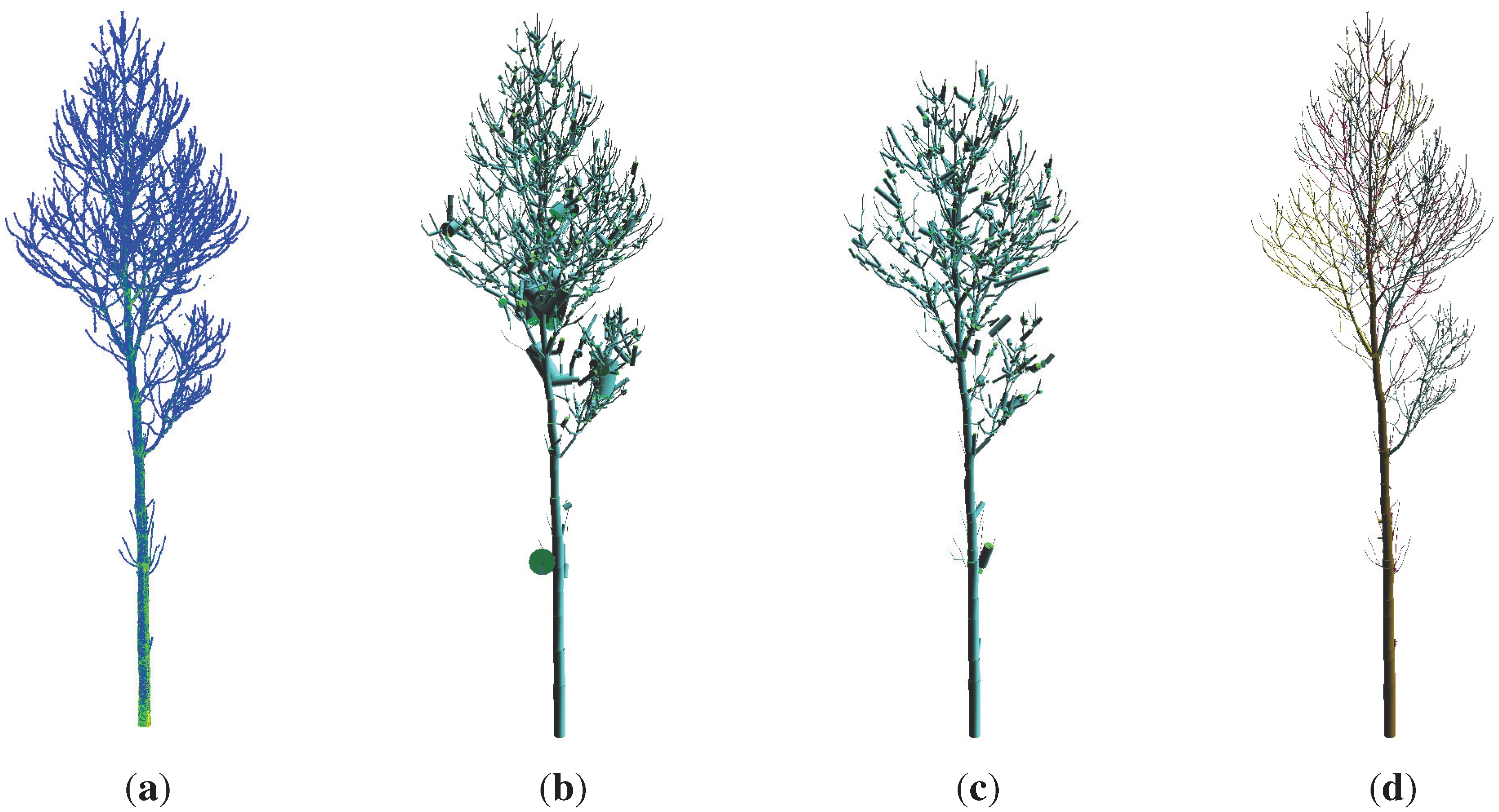
First, a discussion on the impact of the selection of one of the three different circle fitting methods (refer to
Section 4.6) is applied. Visual inspection, as depicted in
Figure 5(b), indicates that the least squares method alone is capable of detecting nearly every branch within the tree; nevertheless, the method still leads to occasional, obviously too large incorrect cylinders. In
Figure 5(c), representing the plane fitting method, the errors are smaller, but the method is not capable of detecting every branch on the tree. The circle fitting method used throughout the results in this paper is the quantile method, which is capable of following every branch without the erroneous results provided by the least squares method. It should be noted that the errors produced in the first (NLS fitting) and the second (plane fitting) method could be minimized with manual threshold adjustment, but never completely eradicated. In public releases of the software, it is intended to include all three circle fitting methods, with an option for the user to choose between them.
Figure 5.
Impact on the selection of different circle fitting methods of tree #1 (height ≈ 12 m): (a) the input point cloud of Tree 1; colors represent (unused) intensity values; (b) a model derived by the NLS method with large failure cylinders; (c) a model derived by the plane fitting method with failure cylinders; (d) a model derived by the quantile method covering the complete input point cloud without errors, with successfully detected stem and branches colored differently.
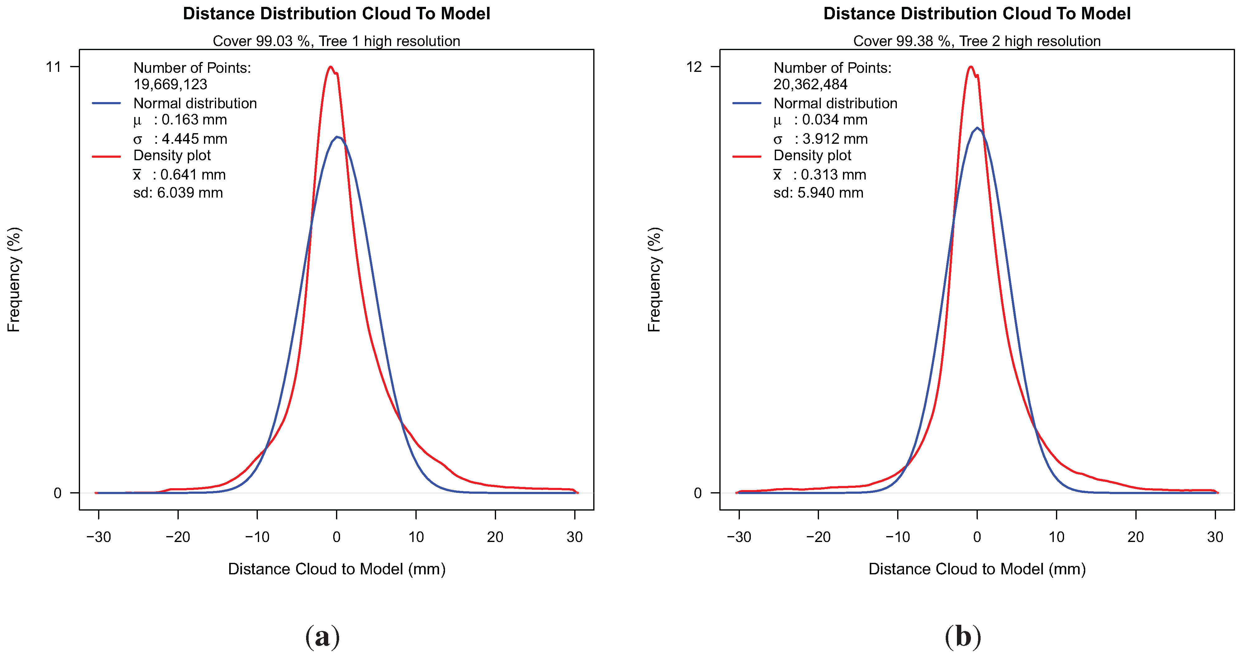
Distance analysis (refer to
Section 4.8) derived plots of the histograms and fitted distributions are depicted in
Figure 6 for both tree models.
Figure 6.
Distance histogram with fitted normal distribution for both Group II point clouds: (a) distance histogram for Tree 1; (b) distance histogram for Tree 2.
Figure 6.
Distance histogram with fitted normal distribution for both Group II point clouds: (a) distance histogram for Tree 1; (b) distance histogram for Tree 2.
In both density plots, two peaks are visible. We attributed the left peak to the least squares fitted parts of the tree and the smaller right peak to the quantile cylinder fitting method. Resulting values for both trees are given for two resolutions; lower resolutions were produced artificially with Laser Control [
41] and noted in
Table 4. For the two high resolution results, we achieved a cover of more than 99%. By reducing the point density by a factor of ten, we had in both results a cover loss of approximately 2%. The average fit quality represented by
x and
μ in every case presented sub-millimeter accuracy. The variance of distances, presented by
sd and
σ, is high compared to the average fit accuracy, this may be attributed to the fact that natural branch segments differ greatly from a mathematical cylinder. Variance also increased with reduced point cloud density. The data preparation with Laser Control was time consuming for the two trees scanned in ultra-high resolution, with total scan file sizes of 36 GB. The software runtime changed from 491 seconds to 41 seconds for Tree 1 by reducing the resolution.
Table 4.
The impact of lowering the point cloud density on the goodness of fit.
Table 4.
The impact of lowering the point cloud density on the goodness of fit.
| Tree ID | Number of Points | sd (mm) | x(mm) | σ (mm) | μ(mm) | Cover (%) |
|---|
| 1 | 19,669,123 | 6.04 | 0.64 | 4.45 | 0.16 | 99.03 |
| 1 | 1,688,509 | 6.09 | 0.79 | 4.47 | 0.28 | 97.04 |
| 2 | 20,362,484 | 5.94 | 0.31 | 3.91 | 0.03 | 99.38 |
| 2 | 2,618,278 | 6.10 | 0.68 | 3.99 | 0.22 | 97.74 |
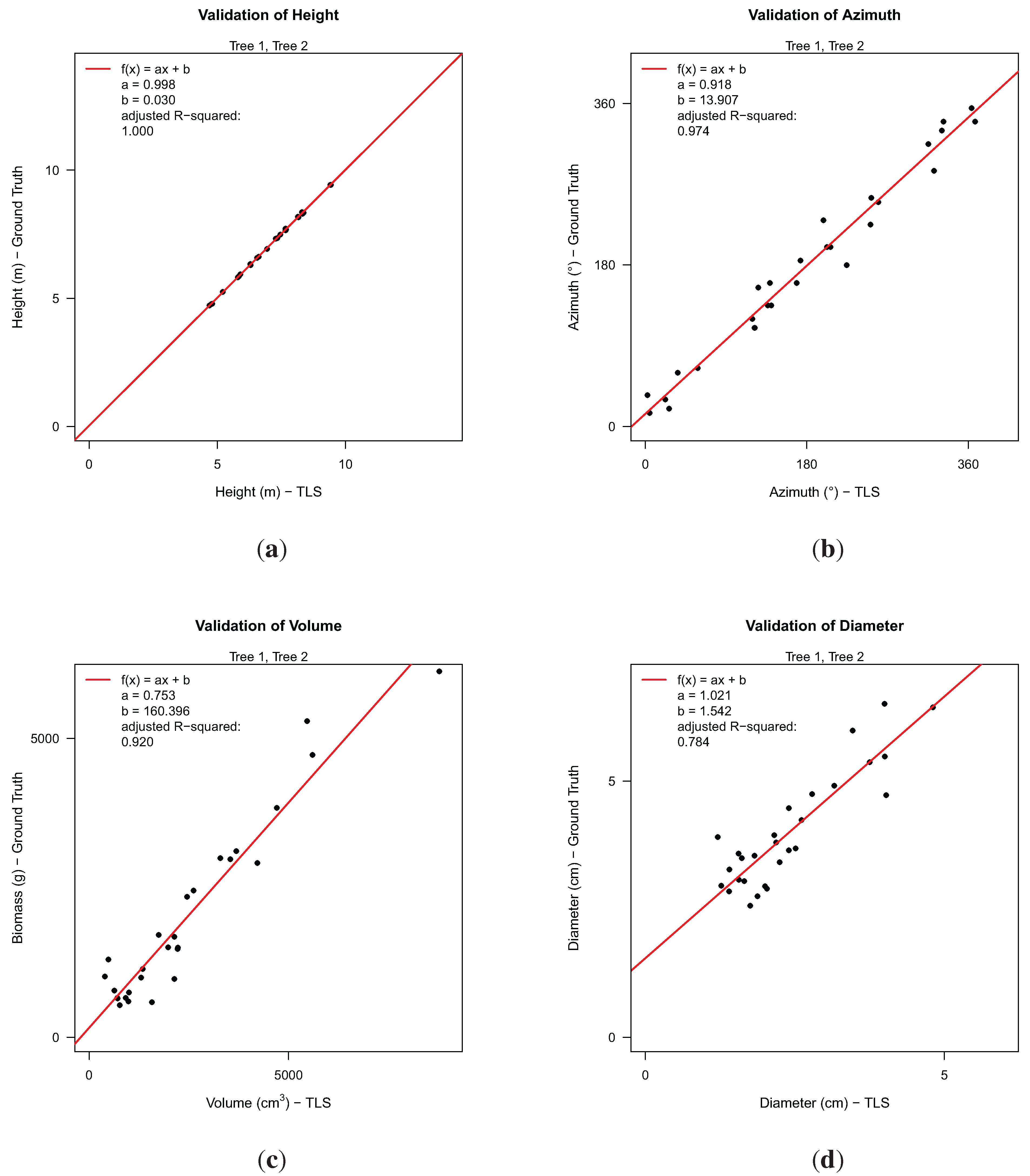
Additionally, comparisons to ground truth measurements were applied, which can be seen in
Figure 7.
Figure 7.
Analysis between TLS-derived data and ground truth data for 28 branches with respect to: (a) branch height; (b) azimuthal direction of branches; (c) TLS-volume against biomass (fresh weight); (d) diameter at branch collar.
Figure 7.
Analysis between TLS-derived data and ground truth data for 28 branches with respect to: (a) branch height; (b) azimuthal direction of branches; (c) TLS-volume against biomass (fresh weight); (d) diameter at branch collar.
From a total of 29 larger branches, 28 could be successfully detected in our resulting data according to height and azimuth. For these branches, we analyzed the correlation between manually-measured and TLS-derived height, the correlation of both azimuth measurements, the correlation between TLS-derived volume and fresh weight and the correlation of diameters at the branch collar. Branch height showed a
![Forests 05 01069 i005]()
equaling 1.000, suggesting that both ground truth and TLS data seem to be measured accurately. For the azimuthal direction, the acquisition of ground truth data was reported to be rather difficult on a standing tree. The coefficient,
a, in the linear model (
![Forests 05 01069 i005]()
= 0.974) with a value of 0.918 might be an indicator of an error in the manual measurements, as visual inspection of TLS results showed no errors regarding the azimuth. As there was no ground truth volume data collected for the branches, it was only possible to model the relation between volume and weight. Density is considered to vary within and between trees [
54]; the resulting
![Forests 05 01069 i005]()
might be expected to be slightly lower. Linear modeling resulted with a
![Forests 05 01069 i005]()
value of 0.92. The largest discrepancy between ground truth data and TLS results was detected in the diameter analysis with a
![Forests 05 01069 i005]()
of 0.784. This discrepancy can be partially explained by two different measurement methods. Ground truth diameters have been measured at the outer extremity of the branch collar. In the TLS method, the diameter of the third cylinder of every branch was taken, as cylinders near branch junctions showed larger errors in diameter than others by visual inspection.
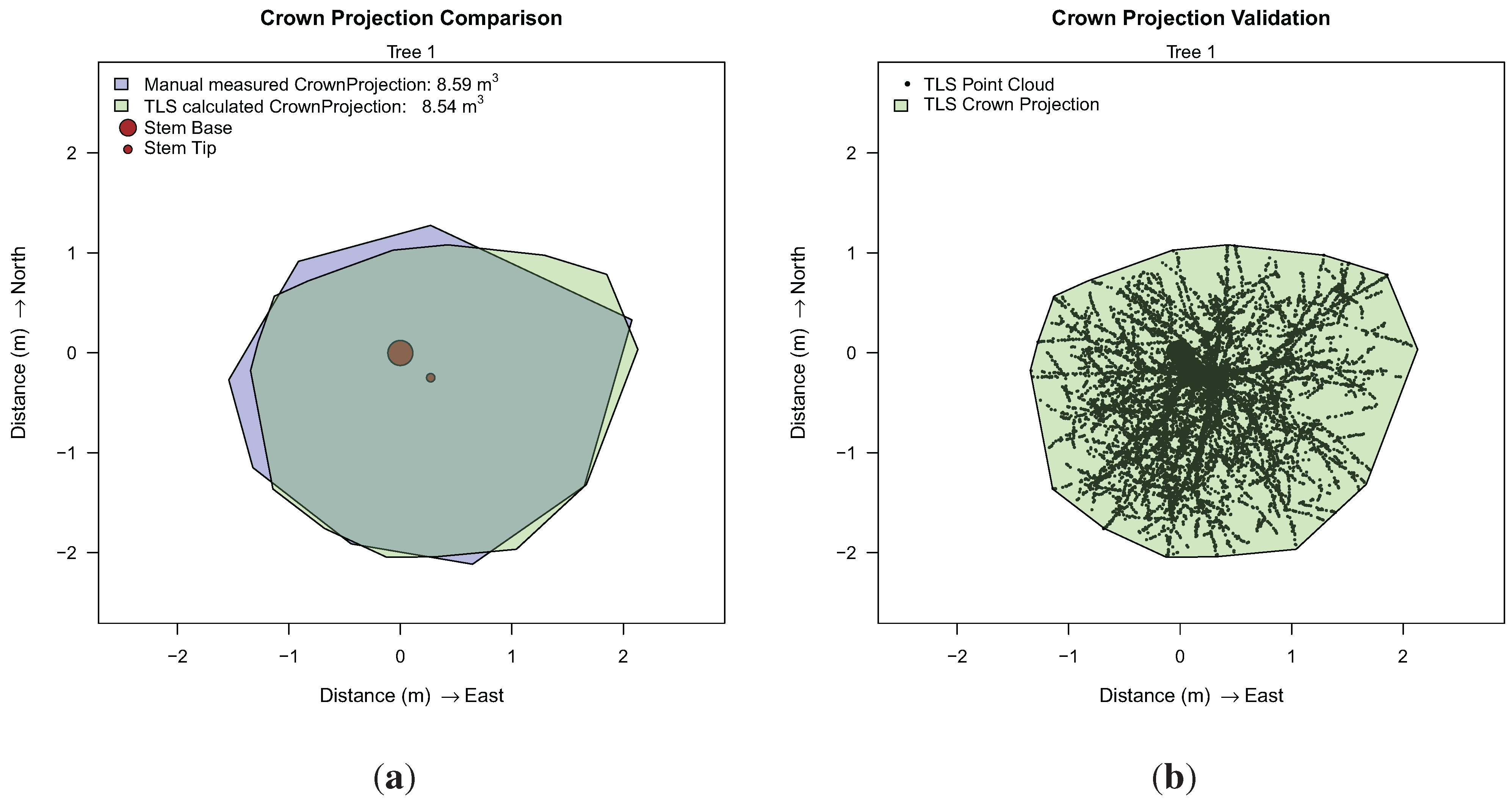
Additionally, a comparison between the manual an TLS-derived crown-projection area was performed for both trees, depicted for Tree 1 in
Figure 8.
Figure 8.
Crown projection analysis for Tree 1: (a) comparison to manual results; (b) in the x,y-plane projected point cloud as visual validation.
Figure 8.
Crown projection analysis for Tree 1: (a) comparison to manual results; (b) in the x,y-plane projected point cloud as visual validation.
Results of the crown projection area, DBH and length measurements are included in
Table 5, showing high accuracy in length measurements. DBH and crown projection area correlate well for Tree 1 with a larger deviation for Tree 2. Visualization of TLS derived results did not reveal an explanation for the deviation, but this might be dictated by the fact that the TLS-derived diameter is taken from a cylinder with a length larger than 20 cm, which still covers the DBH height, but also covers sections below and above 1.3 m. An error in ground truth data or an error caused by the deviation of the stem form from a circular cylinder can also not be suspended.
Table 5.
Comparison of manual ground truth data with the TLS-derived results.
Table 5.
Comparison of manual ground truth data with the TLS-derived results.
| Tree ID | Method | DBH (cm) | Length (m) | Crown projection area (m2) |
|---|
| 1 | manual | 18.6 | 11.52 | 8.59 |
| 1 | TLS | 18.1 | 11.57 | 8.54 |
| 2 | manual | 20.0 | 12.60 | 10.70 |
| 2 | TLS | 21.4 | 12.62 | 12.00 |
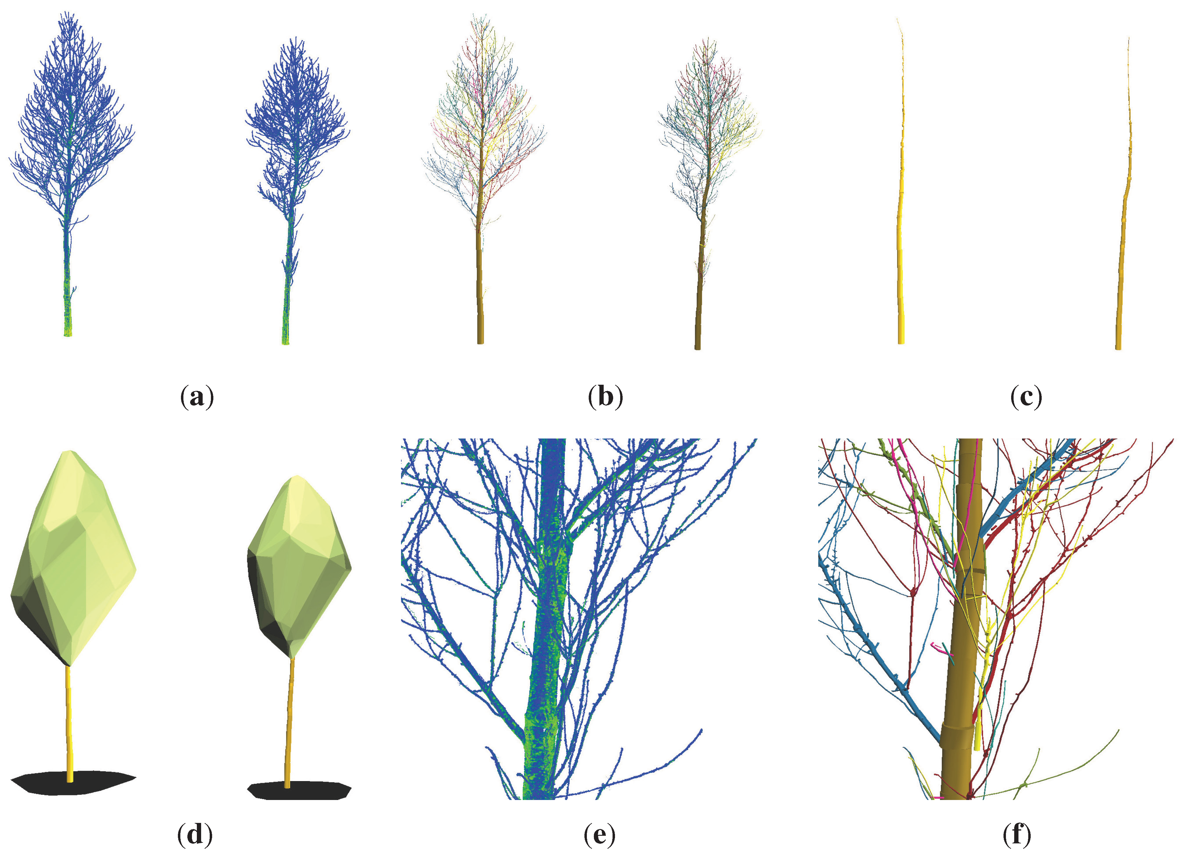
Visualization of the cylinder models of both trees are depicted in
Figure 9.
Figure 9.
Visualization of both Group II trees (height ≈ 12 m): (a) TLS point clouds; (b) cylinder models with branches colored differently; (c) extracted stems of the cylinder models; (d) model of the crowns, stems and crown projections; (e) enlarged view into the lower crown point cloud of 2; (f) enlarged view into the lower crown cylinder model of 2.
5.3. Artificial Point Cloud Results
Thresholds used for Groups II and III could not be applied to the artificial point cloud. It took about 20 software runs to adjust the thresholds to a point where satisfactorily results were achieved (refer to
Figure A1). Comparisons between the values of the original cylinder model and that derived by our software are included in
Table 6. An underestimation of the crown projection area by our method indicates that not every branch was followed to its tip. With an overestimation of 2.5% of total volume, either some incorrect cylinders were included in our model or the diameter of cylinders was slightly overestimated. Visualization showed for this point cloud that, due to the very dense neighborhood of small branches, sometimes artificial connections between two branches are included in our model. Distance analysis with values given in
Table 7 indicates a good cover of our model: missing only 0.5% of the point cloud. This suggests that the algorithm is suitable for a wider range of tree forms than just
P. avium [
55]. Better variance parameters than those found for the ground truth trees are possible due to the mathematical origin of the point cloud data, while
x results in poorer values than for the same parameter for the Group II trees.
Table 6.
Comparison between original data and the proposed method results for the artificial point cloud.
Table 6.
Comparison between original data and the proposed method results for the artificial point cloud.
| Data Set | DBH (cm) | height (m) | Volume (L) | Crown Projection Area (m2) |
|---|
| original | 22.4 | 17.73 | 666.5 | 30.81 |
| program results | 22.4 | 17.74 | 683.6 | 29.70 |
Table 7.
Distance analysis between the point cloud and the derived model for the artificial tree.
Table 7.
Distance analysis between the point cloud and the derived model for the artificial tree.
| Tree ID | Number of Points | sd (mm) | x (mm) | σ (mm) | μ (mm) | Cover (%) |
|---|
| artificial | 3,442,699 | 5.00 | 2.134 | 2.13 | 0.07 | 99.48 |
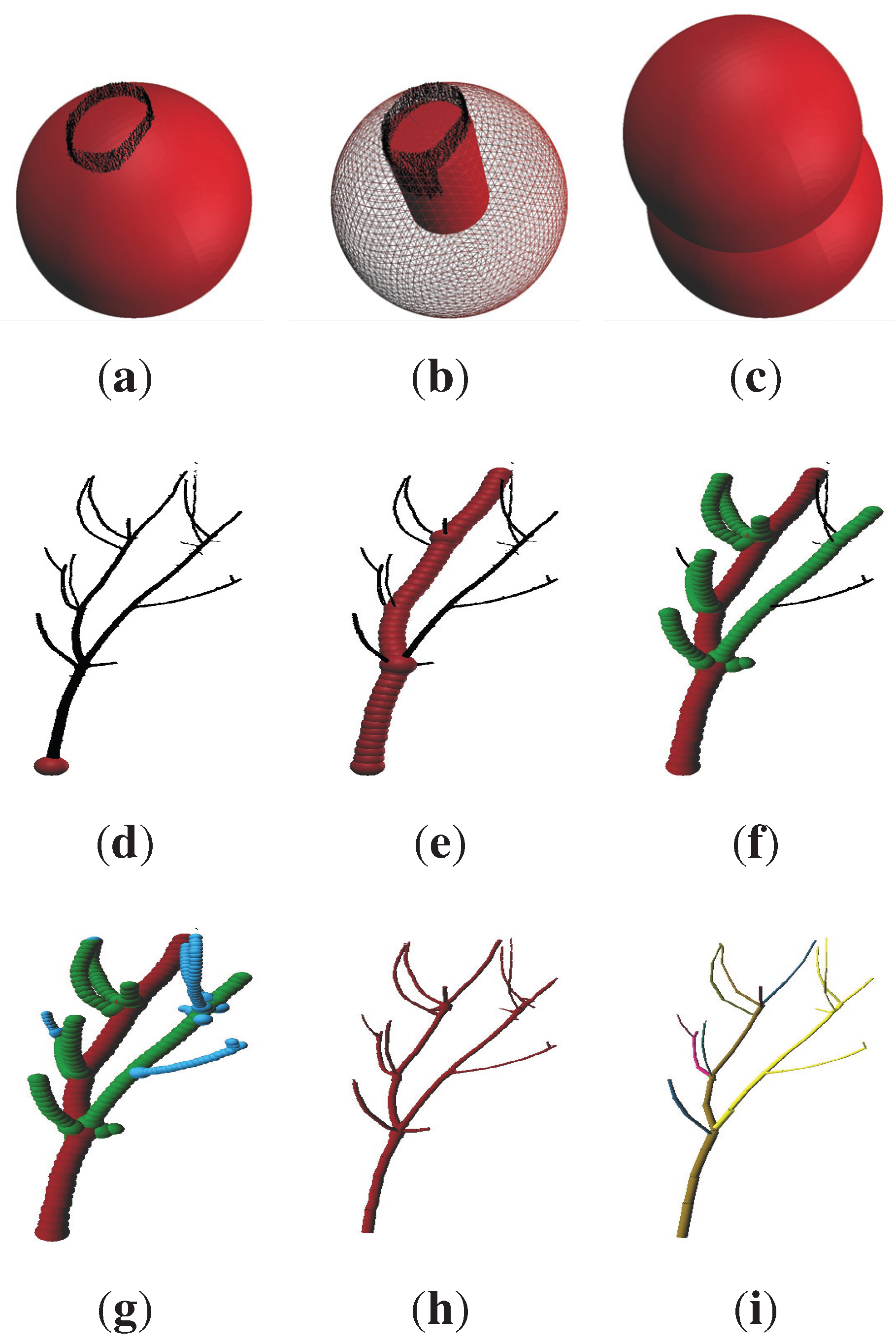
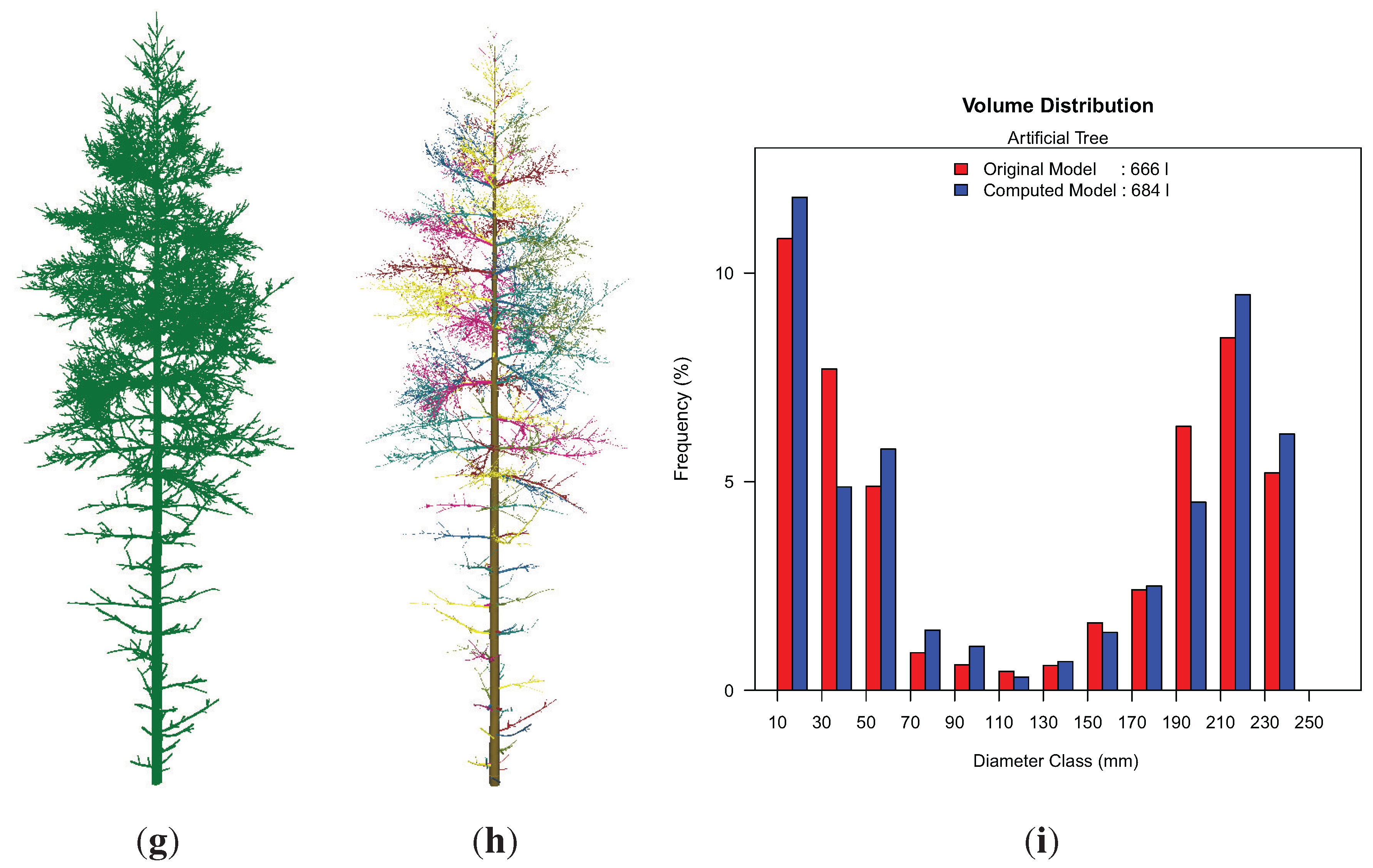
Visualization of the results of the artificial point cloud (
Figure 10(g)) is depicted in
Figure 10(h),(i), showing a histogram of the volume distribution according to the diameter of the cylinders. While most diameter classes are well represented in this histogram, the 180–200 mm class is largely underestimated. We suppose, as this class is located in part of the stem, where many branch junctions are growing, that some cylinders’ diameters in the area of branch junctions are overestimated, due to the allocation of branch points to the stem cylinder before a least squares fit is applied. These cylinders are then classified into the next two larger diameter classes, leading to the depicted overestimation of total volume in these classes.
Both our method and the one of Raumonen
et al. [
32] are able to reconstruct height and volume very accurately (
i.e., the error is within a few percent) [
56].
5.4. Group III Results
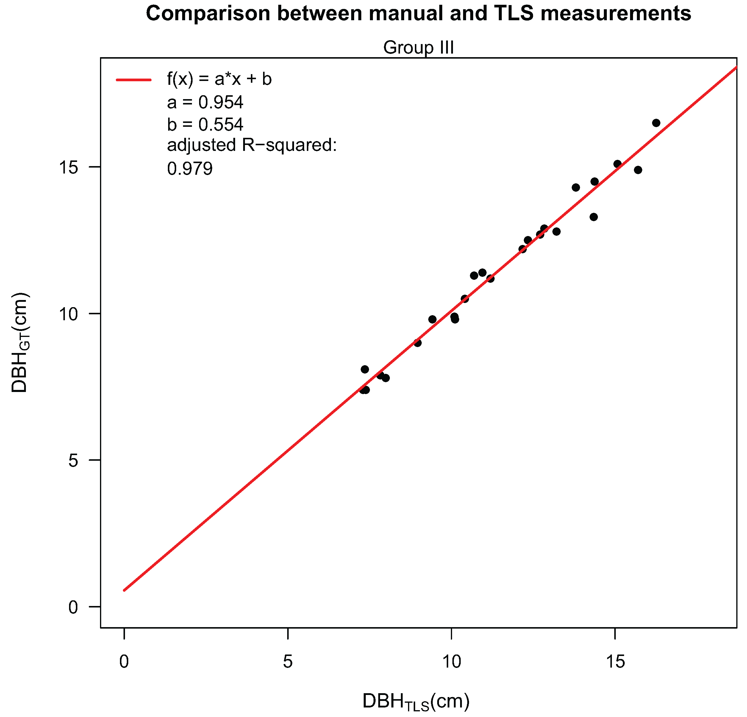
Using a loop, the total runtime for all 24 extracted trees was less than 30 min in total. Results for distance analysis, DBH and volume are given in
Table 8. This table also includes ground truth DBH measurements, and a comparison of the two different DBH values is performed in
Figure 11. The derived linear model shows a
![Forests 05 01069 i005]()
value of 0.979.
Table 8.
Partial results for 24 Group III trees.
Table 8.
Partial results for 24 Group III trees.
| ID | Points | DBHTLS(GT)1 (cm) | Vol(l) | sd (mm) | x (mm) | σ (mm) | μ (mm) | Cover (%) |
|---|
| 3 | 503,794 | 10.69 (11.3) | 64.24 | 5.39 | 1.11 | 3.61 | 0.30 | 81.01 |
| 4 | 1,750,783 | 16.25 (16.5) | 164.30 | 5.80 | 1.35 | 4.51 | 0.57 | 94.24 |
| 5 | 1,033,913 | 8.96 (9.0) | 54.40 | 5.24 | 1.31 | 3.45 | 0.41 | 97.99 |
| 6 | 1,901,388 | 14.38 (14.5) | 139.96 | 5.79 | 1.69 | 4.34 | 0.78 | 86.84 |
| 7 | 1,091,585 | 14.35 (13.3) | 122.11 | 7.36 | 1.96 | 5.77 | 1.01 | 78.03 |
| 8 | 722,546 | 10.41 (10.5) | 65.21 | 6.27 | 1.77 | 4.52 | 0.78 | 86.16 |
| 9 | 1,289,349 | 15.08 (15.1) | 140.82 | 5.39 | 1.19 | 3.65 | 0.31 | 78.82 |
| 10 | 604,092 | 7.83 (7.9) | 34.53 | 4.90 | 1.07 | 2.97 | 0.23 | 88.05 |
| 11 | 2,414,504 | 15.70 (14.9) | 159.42 | 5.93 | 1.73 | 3.99 | 0.67 | 82.12 |
| 12 | 1,332,867 | 13.80 (14.3) | 131.83 | 6.41 | 1.77 | 4.47 | 0.73 | 84.05 |
| 13 | 1,241,908 | 12.84 (12.9) | 109.74 | 6.04 | 1.57 | 4.08 | 0.48 | 90.00 |
| 14 | 645,269 | 10.09 (9.9) | 62.17 | 5.84 | 1.44 | 3.64 | 0.38 | 88.04 |
| 15 | 1,289,349 | 10.11 (9.8) | 49.28 | 6.58 | 1.95 | 3.78 | 0.62 | 71.80 |
| 16 | 523,777 | 7.36 (8.1) | 32.74 | 5.58 | 1.44 | 3.55 | 0.48 | 97.38 |
| 17 | 1,743,865 | 12.18 (12.2) | 102.83 | 5.35 | 1.47 | 3.69 | 0.57 | 92.16 |
| 18 | 1,316,364 | 12.71 (12.7) | 96.06 | 5.51 | 1.64 | 3.73 | 0.68 | 79.26 |
| 19 | 649,161 | 10.95 (11.4) | 58.93 | 5.38 | 1.06 | 3.71 | 0.31 | 93.10 |
| 20 | 933,400 | 13.21 (12.8) | 91.17 | 5.40 | 1.48 | 3.63 | 0.54 | 88.62 |
| 21 | 266,787 | 7.30 (7.4) | 22.85 | 5.30 | 1.39 | 2.85 | 0.34 | 84.19 |
| 22 | 355,830 | 7.99 (7.8) | 27.65 | 5.27 | 1.29 | 2.84 | 0.26 | 77.52 |
| 23 | 1,074,614 | 12.34 (12.5) | 80.72 | 5.92 | 1.81 | 3.85 | 0.72 | 89.03 |
| 24 | 674,759 | 11.90 (11.2) | 74.51 | 5.77 | 1.27 | 4.24 | 0.40 | 96.51 |
| 25 | 373,704 | 7.39 (7.4) | 28.16 | 5.21 | 1.36 | 3.33 | 0.49 | 92.30 |
| 26 | 410,720 | 9.42 (9.8) | 40.33 | 5.61 | 1.62 | 3.46 | 0.50 | 77.60 |
| mean | 1,006,255 | 11.36 (11.43) | 81.41 | 5.72 | 1.49 | 3.82 | 0.52 | 86.45 |
Although the average cover for the 24 models is only 86.45%, which naturally enlarges the parameter, x, parameters of the fitted normal distribution, σ and μ, were comparable to those of Group II models.
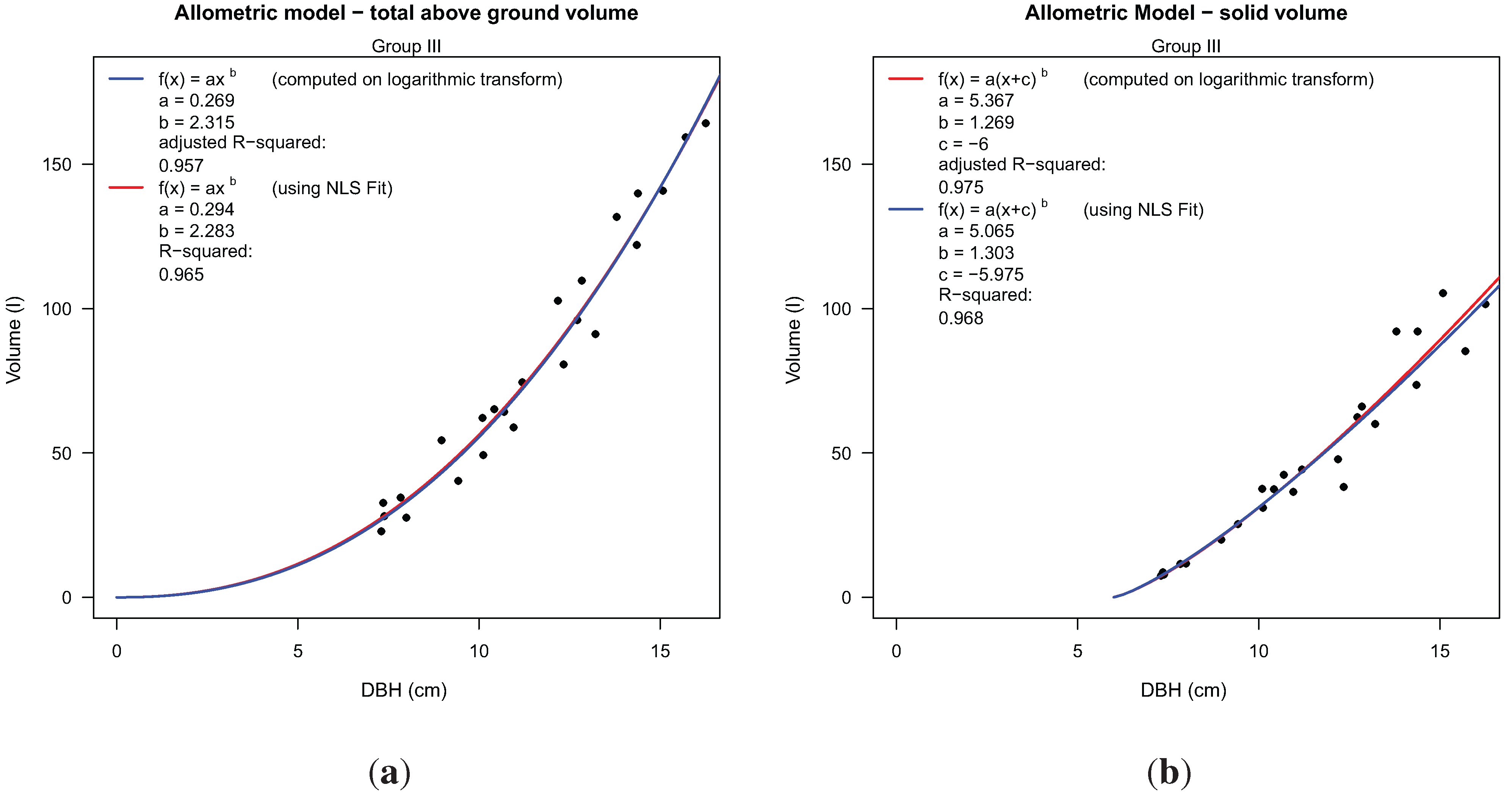
We were able to build two allometric models using DBH as a predictor variable, as an example of the more general use of the reconstructed 3D tree information. The number of samples (24) is still too low to use these example allometric models in forestry applications.
Total above ground volume is derived from Equation (1); the volume of woody segments with diameter larger than 7 cm (solid volume) utilized a modified equation, as given in
Figure 12(b). Modification of the equation was performed to prevent the prediction of solid volume for trees from being too small to contain solid segments. Models showed values for r
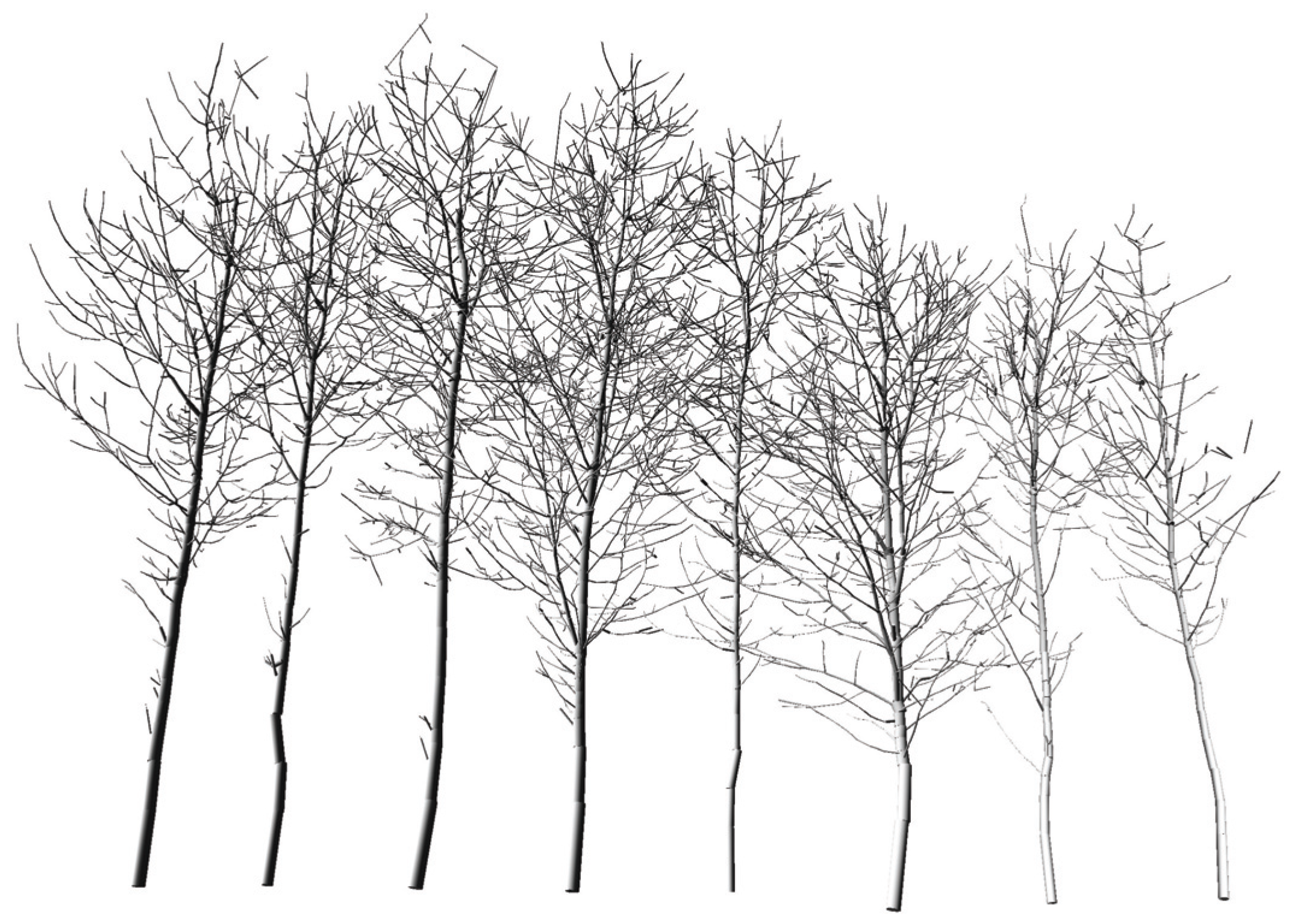
2 equaling 0.965 and 0.968, respectively. A visualization of a group of eight neighboring trees can be seen in
Figure 3, depicting overlapping crowns. Low scan resolution together with occlusion effects causes a low density of data points, leading to incorrectly modeled branches located in the upper crowns.
Figure 10.
Visualization of the artificial tree results (height ≈ 18 m): (g) artificial point cloud; (h) resulting cylinder model with branches colored differently; (i) volume distribution in both the original data and program results.
Figure 10.
Visualization of the artificial tree results (height ≈ 18 m): (g) artificial point cloud; (h) resulting cylinder model with branches colored differently; (i) volume distribution in both the original data and program results.
Figure 11.
Validation of TLS-derived and manually-measured DBH measurements.
Figure 11.
Validation of TLS-derived and manually-measured DBH measurements.
Figure 12.
Two allometric models for volume estimation derived from 24 Group III models using TLS-derived DBH as the input variable: (a) total above-ground volume modeled as a function of DBH; (b) solid volume modeled as a function of DBH.
Figure 12.
Two allometric models for volume estimation derived from 24 Group III models using TLS-derived DBH as the input variable: (a) total above-ground volume modeled as a function of DBH; (b) solid volume modeled as a function of DBH.

 ,
, 

 and
and  of the branch volume was covered. In addition, a comparison between modeled and manually measured diameters was performed.


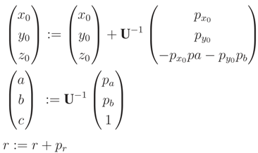
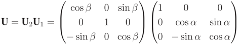
 the normalized direction vector of the next cylinder in the segment:
 (n#h) (#h being the number of hull faces), terminated in less than a second.
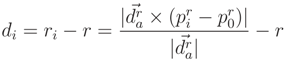
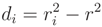
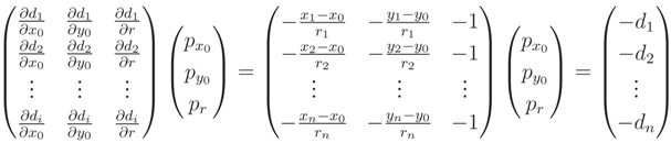
 = (a, b, c)T the direction vector of ax and r the cylinder radius. The implementation details of the applied Gauss–Newton algorithm [53] are given in Appendix B.1.
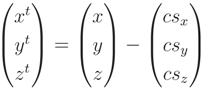
 , of pi onto the cylinder axis is between start point cs and end point ce of the cylinder. Else, we define
  in Equation (9):


 ) = 0.95) points to a slight underestimation of the volume within the TLS results.
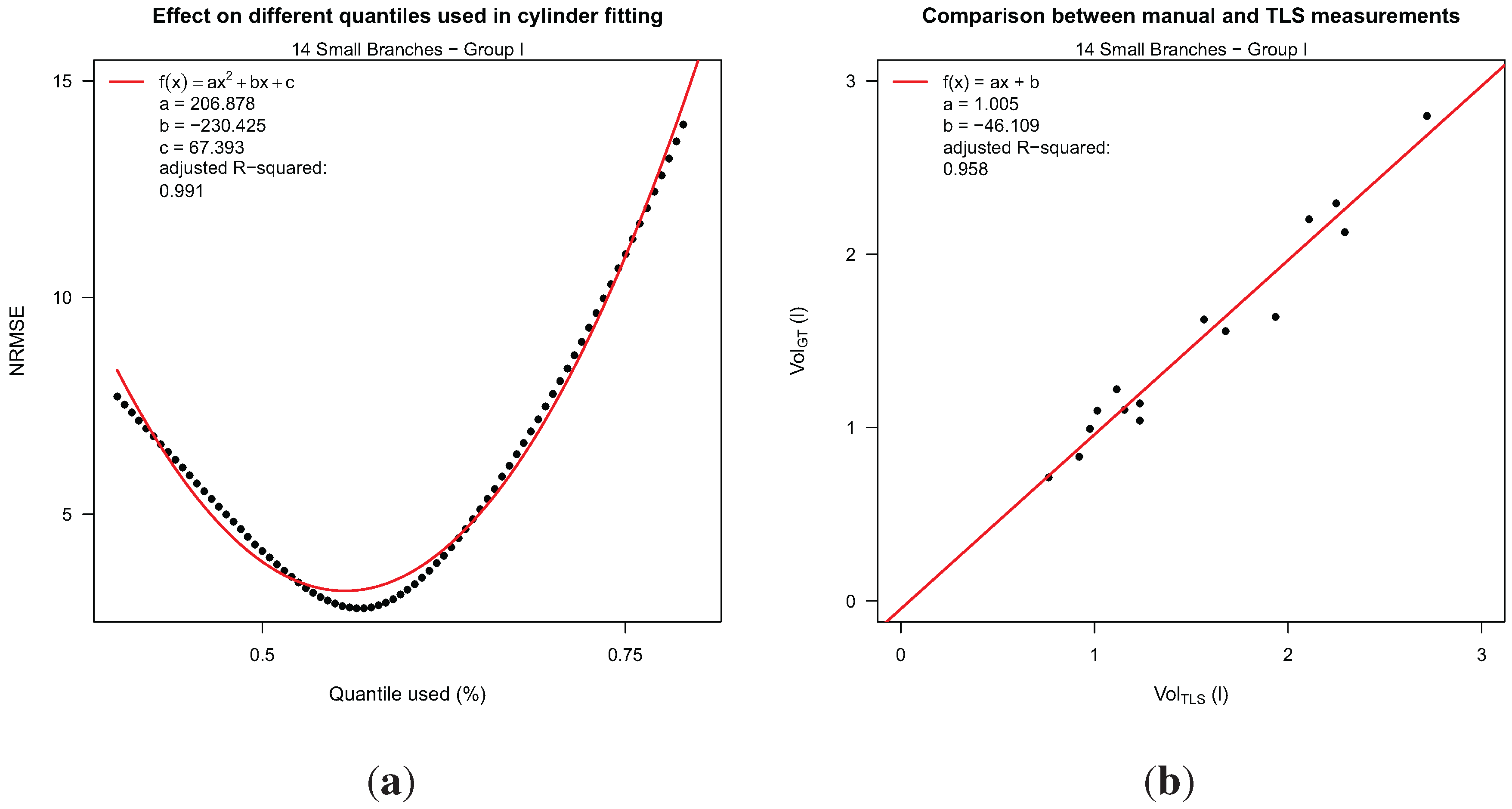


 being the Jacobian matrix.

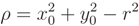
 with
with  , we define distance di of a point,
  , to the cylinder in Equation (A4):
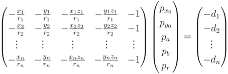
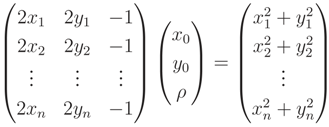

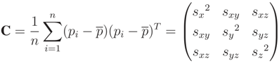
 , satisfying the linear Equation (A16), where λi are the eigenvalues corresponding to each
  .
.