Assessing the Potential Stem Growth and Quality of Yellow Birch Prior to Restoration: A Case Study in Eastern Canada


Abstract
:1. Introduction
2. Experimental Section
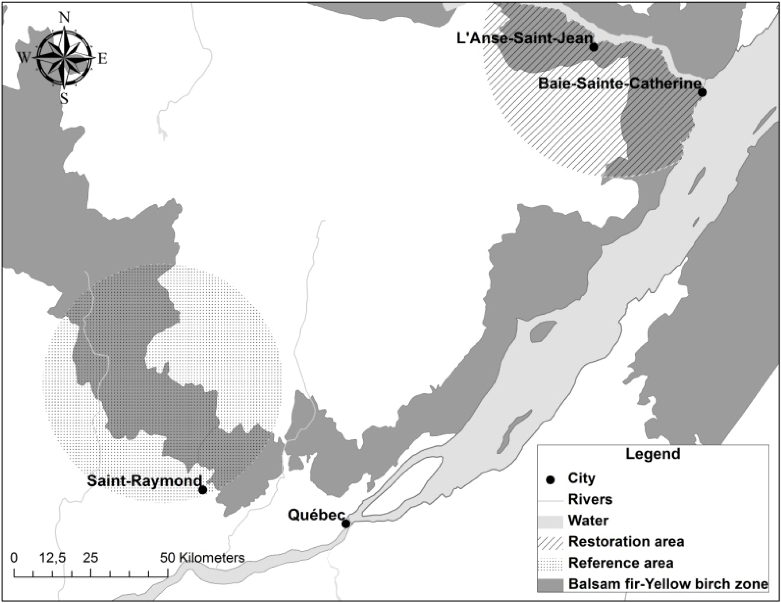
2.1. Field Sampling

| Area | Number of TSPs | Number of trees (cm) | DBH (cm) | H (m) | d2h (m3) | Age (years) | BAI5Y (cm2/5 years) | SLC4F (m) |
|---|---|---|---|---|---|---|---|---|
| Reference | 22 | 76 | 3.7–67.5 | 6.1–24.6 | 0.01–8.06 | 14–231 | 43.7 (32.2) | 9.7 (4) |
| Restoration | 19 | 66 | 2.5–53.2 | 2.73–20 | 0–4.78 | 16–229 | 34.7 (26.8) | 8.3 (3.6) |
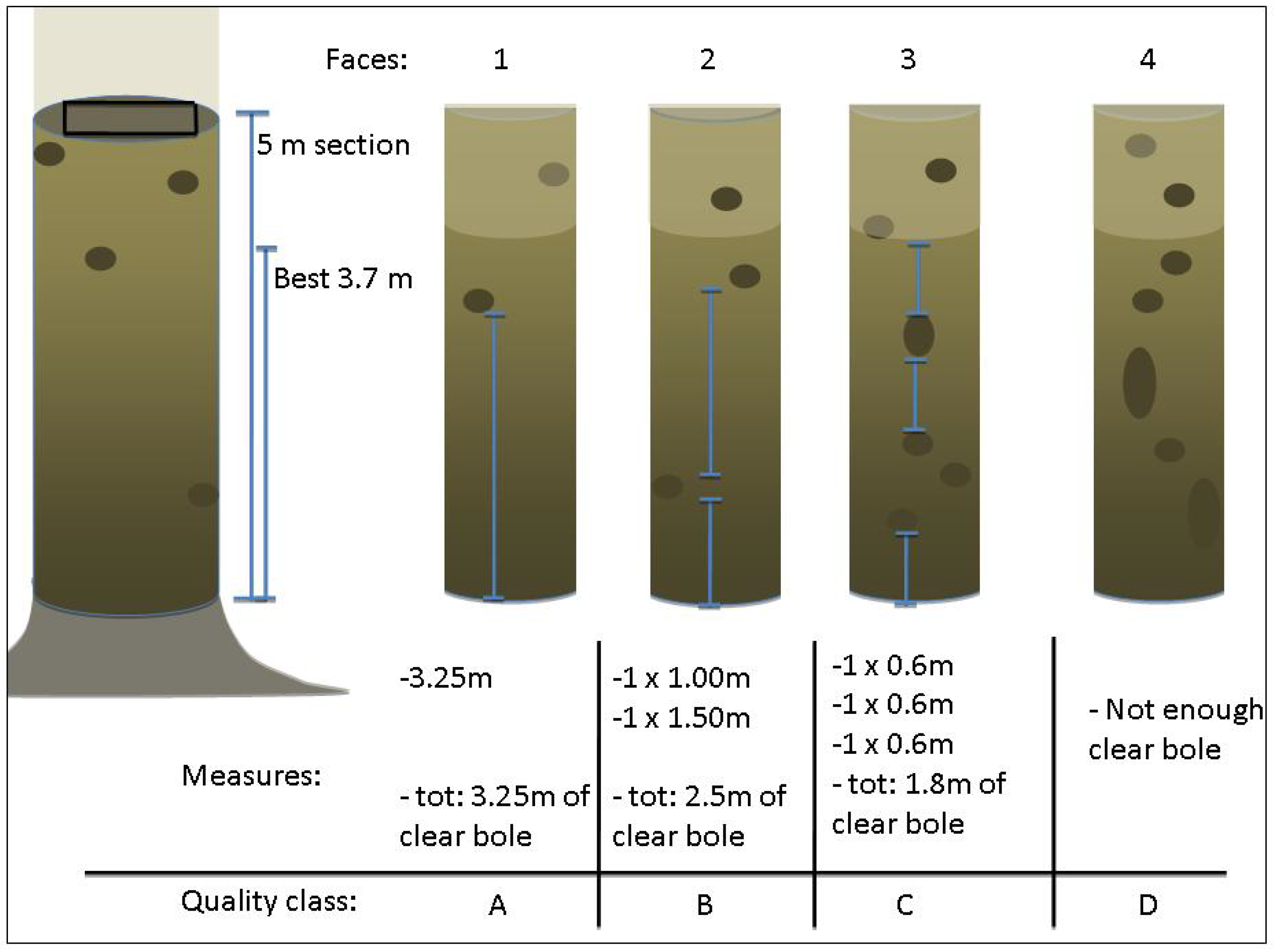
2.2. Stem Growth and Quality Assessments

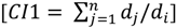
2.3. Independent Variables
| Area | Degree Days (°C/year) | Growing Season (days) | Temp. Daily Min (°C) | Temp. Daily Mean (°C) | Temp. Daily Max (°C) | Precipitations (mm) | Altitude (m) | CI1 | CI2 | Site Index | Main Competitor species | |
|---|---|---|---|---|---|---|---|---|---|---|---|---|
| Reference | 2154 (145) | 134 ** (9) | −4.8 ** (0.8) | 1.3 ** (0.7) | 7.4 ** (0.6) | 1317 ** (62) | 492 ** (118) | 9.6 ns (10.5) | 3.5 ns (5.6) | 11.6 * (0.8) | CYB: | 33 |
| M: | 6 | |||||||||||
| O: | 37 | |||||||||||
| Restoration | 2262 (69) | 151 ** (8) | −3.5 ** (0.8) | 1.8 ** (0.5) | 7.1 ** (0.3) | 1034 ** (26) | 288 ** (86) | 9.9 ns (13) | 4 ns (6) | 11.4 * (0.7) | CYB: | 32 |
| M: | 9 | |||||||||||
| O: | 25 | |||||||||||
2.4. Model Development


3. Results
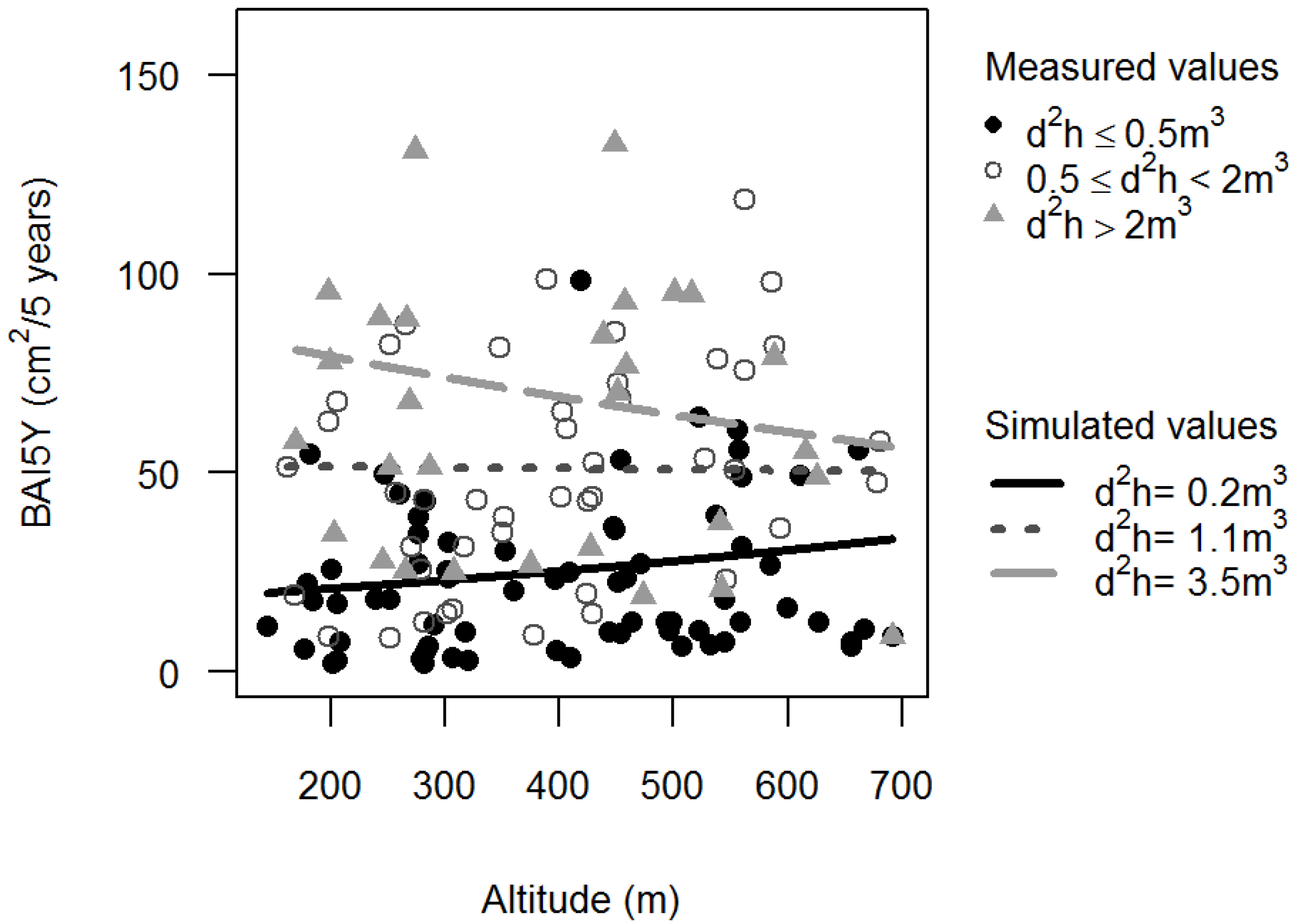
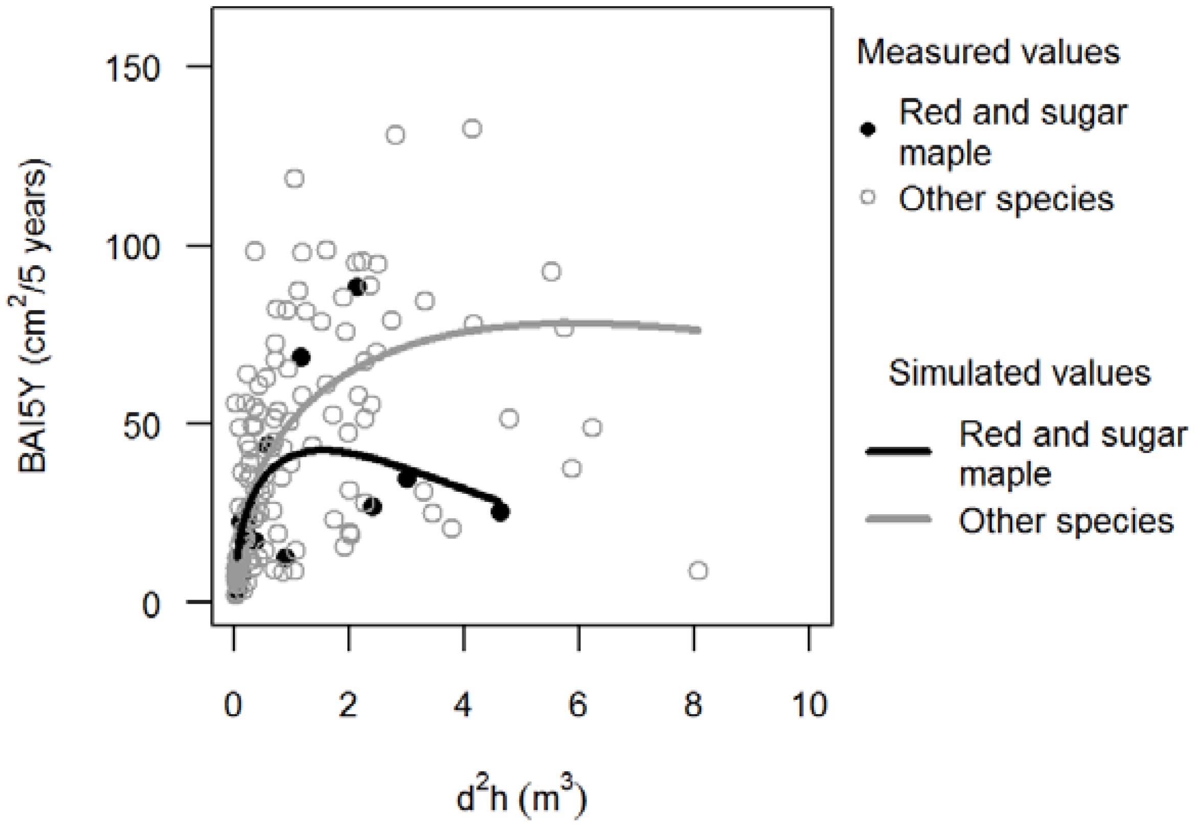
3.1. Basal Area Increments

 ,
,  ).
). : Mean Absolute Error relative to the observed mean. Step 1: fixed-effects model; Step 2: random effects model; Step3: random-effects model with selected covariates; Step 4: random effects model with covariates and selected random effects.
| Step | a0 | b0 | b1 | c0 | c1 | σplot (α0j) | σplot (β0j) | σplot (γ0j) | εij | AIC | RMSE | MAE | MAE% | EF |
|---|---|---|---|---|---|---|---|---|---|---|---|---|---|---|
| cm2/5 years | cm2/5 years | % | ||||||||||||
| 1 | 64.6 ** (6.8) | 0.5 ** (0.1) | 0.8 ** (0.05) | 21.4 | 1307.6 | 23.7 | 17.7 | 44.8 | 0.38 | |||||
| 2 | 54.0 ** (5.8) | 0.4 ** (0.1) | 0.9 ** (0.05) | 16 | 5.0 × 10⁻⁵ | 2.9 × 10⁻⁵ | 21.3 | 1284.6 | 18.4 | 14.0 | 35.3 | 0.63 | ||
| 3 | 55.2 ** (5.7) | 0.7 ** (0.1) | 0.7 ** (2.2−4) | 0.7 ** (0.08) | 0.9 ** (0.08) | 16.9 | 4.0 × 10⁻⁵ | 3.0 × 10⁻⁶ | 19.9 | 1274.4 | 16.8 | 13.1 | 33.1 | 0.69 |
| 4 | 55.1 ** (5.7) | 0.7 ** (0.7) | 0.7 ** (2.2−4) | 0.7 ** (0.08) | 0.9 ** (0.09) | 16.9 | 19.9 | 1264.4 | 16.8 | 13.1 | 33.2 | 0.69 |
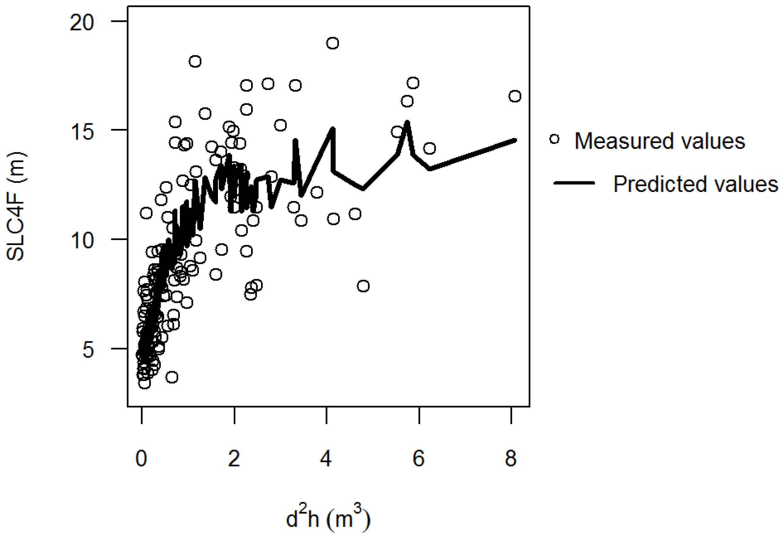
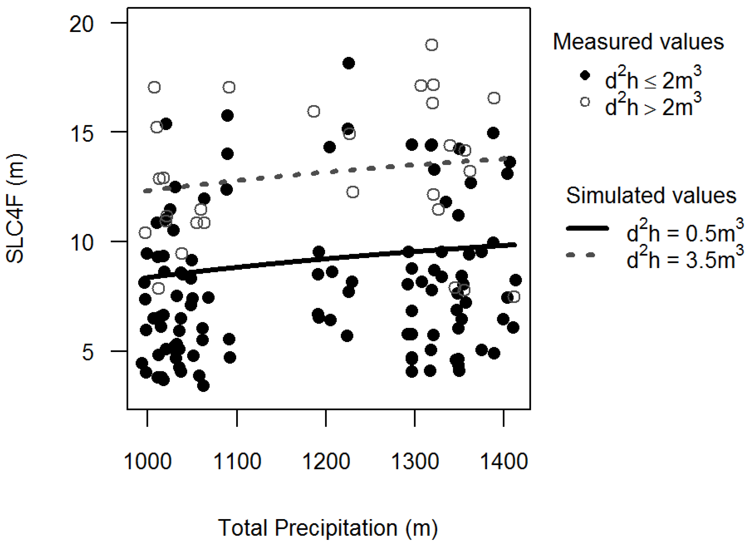
3.2. Stem Quality

 : Mean Absolute Error relative to the observed mean. Step 1: fixed-effects model; Step2: random effects model; Step3: random-effects model with selected covariates; Step 4: random effects model with covariates and selected random effects.
| Step | a0 | a1 | b0 | c0 | σplot (α0j) | σplot (β0j) | σplot (γ0j) | εij | AIC | RMSE | MAE | MAE% | EF |
|---|---|---|---|---|---|---|---|---|---|---|---|---|---|
| m | m | % | |||||||||||
| 1 | 5.5 ** (0.4) | 9.3 ** (0.7) | −0.6 ** (0.1) | 2.4 | 657.1 | 2.4 | 1.9 | 21.0 | 62.0 | ||||
| 2 | 5.3 ** (0.2) | 8.9 ** (0.7) | −0.5 ** (0.07) | 3.3 × 10⁻⁴ | 1.7 | 1.0 × 10⁻⁶ | 2.4 | 642.7 | 2.1 | 1.7 | 18.4 | 70.9 | |
| 3 | 9.6 ** (1.4) | −5120.9 ** (1579.0) | 8.9 ** (0.7) | −0.4 ** (0.07) | 1.6 × 10⁻⁴ | 1.5 | 2.0 × 10⁻⁶ | 2.3 | 634.9 | 2.1 | 1.6 | 18.0 | 71.3 |
| 4 | 9.6 ** (1.4) | −5118.6 ** (1579.1) | 8.9 ** (0.7) | −0.4 ** (0.07) | 1.5 | 2.3 | 630.9 | 2.1 | 1.6 | 18.0 | 71.3 |

4. Discussion
5. Conclusions
Acknowledgments
Conflicts of Interest
References
- Seymour, R.S.; White, A.S.; Demaynadier, P.G. Natural disturbance regimes in northeastern North America—Evaluating silvicultural systems using natural scales and frequencies. For. Ecol. Manag. 2002, 155, 357–367. [Google Scholar] [CrossRef]
- Kneeshaw, D.; Prevost, M. Natural canopy gap disturbances and their role in maintening mixed-species forests of central Quebec, Canada. Can. J. For. Res. 2007, 37, 1534–1544. [Google Scholar] [CrossRef]
- Prévost, M. Effect of cutting intensity on microenvironmental conditions and regeneration dynamics in yellow birch-conifer stands. Can. J. For. 2008, 38, 3317–3330. [Google Scholar]
- Nyland, R.D. Exploitation and greed in eastern hardwood forests—Will foresters get another chance? J. For. 1992, 90, 33–37. [Google Scholar]
- Archambault, L.; Delisle, C.; Larocque, G.R. Forest regeneration 50 years following partial cutting in mixedwood ecosystems of southern Quebec, Canada. For. Ecol. Manag. 2009, 257, 703–711. [Google Scholar] [CrossRef]
- Archambault, L.; Delisle, C.; Larocque, G.R.; Sirois, L.; Belleau, P. Fifty years of forest dynamics following diameter-limit cuttings in balsam fir-yellow birch stands of the Lower St. Lawrence region, Quebec. Can. J. For. Res. 2006, 36, 2745–2755. [Google Scholar] [CrossRef]
- Lorimer, C.G. The presettlement forest and natural disturbance cycle of northeastern Maine. Ecology 1977, 58, 139–148. [Google Scholar] [CrossRef]
- Archambault, L.; Morissette, J.; Bernier-Cardou, M. Forest succession over a 20-year period following clearcutting in balsam fir-yellow birch ecosystems of eastern Québec, Canada. For. Ecol. Manag. 1998, 102, 61–74. [Google Scholar] [CrossRef]
- Aubé, M. The pre-European settlement forest composition of the Miramichi River watershed, New Brunswick, as reconstructed using witness trees from original land surveys. Can. J. For. 2008, 38, 1159–1183. [Google Scholar]
- Crête, M.; Marzell, L. Évolution des forêts québécoises au regard des habitats fauniques: Analyse des grandes tendances sur trois décennies. For. Chron. 2006, 82, 368–382. (in French). [Google Scholar]
- Boucher, Y.; Arsenault, D.; Sirois, K. Logging-induced change (1930–2002) of a preindustrial landscape at the northern range limit of northern hardwoodsm, Eastern Canada. Can. J. For. 2006, 36, 505–517. [Google Scholar]
- Boucher, Y.; Arsenault, D.; Sirois, K.; Blais, L. Logging patterne and landscape changes over the last century at the boreal and deciduous forest transition in Eastern Canada. Landsc. Ecol. 2009, 24, 171–184. [Google Scholar]
- Alvarez, E.; Bélanger, L.; Archambault, L.; Raulier, F. Portrait preindustriel dans un contexte de grande variabilité naturelle: Une étude de cas dans le centre du Québec (Canada). For. Chron. 2011, 87, 612–624. (in French). [Google Scholar]
- Dubois, J.; Ruel, J.C.; Elie, J.-G.; Archambalut, L. Dynamique et estimation du rendement des strates de retour après coupe totale dans la sapinière à bouleau jaune. For. Chron. 2006, 82, 675–689. (in French). [Google Scholar]
- Grondin, P.; Noël, J.; Hotte, D. L’intégration de la végétation et de ses variables explicatives à des fins de classification et de cartographie d’unités homogènes du Québec méridional; (in French). Ministère des Ressources naturelles et de la Faune, Direction de la recherche forestière: Québec, Canada, 2007; p. 80. [Google Scholar]
- Prevost, M.; Dumais, D.; Pothier, D. Growth and mortality following partial cutting in a trembling aspen-conifer stand: Results after 10 years. Can. J. For. Res 2010, 40, 894–903. [Google Scholar] [CrossRef]
- Dupuis, S.; Arseneault, D.; Sirois, L. Change from pre-settlement to present-day forest composition reconstructed from early land survey records in eastern Québec, Canada. J. Veg. Sci. 2011, 22, 564–575. [Google Scholar] [CrossRef]
- Burns, R.M.; Honkala, B.H. Silvics of North America: 1. Conifers; 2. Hardwoods; U.S. Department of Agriculture, Forest Service: Washington, DC, USA, 1990; p. 877. [Google Scholar]
- Coulombe, G.; Huot, J.; Arsenault, J.; Bauce, E.; Bernard, J.-T.; Bouchard, A.; Liboiron, M.-A.; Szaraz, G. Rapport de la Commission d’étude sur la gestion de la forêt publique québécoise; (in French). Commission d’étude sur la gestion de la forêt publique québécoise: Québec, Canada, 2004. [Google Scholar]
- Bureau du Forestier en Chef Résultats (2008–2013) des possibilités annuelles de coupe. Résultats régionaux (fiche synthèse). Available online: http://www.forestierenchef.gouv.qc.ca/ (accessed on 16 April 2013).
- Ministry of Natural Resources and Fauna Québec, Ressources et industries forestières—Portrait Statistique Édition 2012. (in French). MRNFPQ, Direction du développement de l’industrie des produits forestiers: Québec, Canada, 2012; p. 73.
- Godman, R.M.; Krefting, L.F. Factors important to yellow birch establishment in Upper Michigan. Ecology 1960, 41, 18–28. [Google Scholar] [CrossRef]
- Gastellado, P.; Ruel, J.C.; Lussier, J.M. Remise en production des bétulaies jaunes résineuses degrades—Étude du succès d’installation de la régénération. For. Chron. 2007, 83, 742–753. (in French). [Google Scholar]
- Lorenzetti, F.; Delagrange, S.; Bouffard, D.; Nolet, P. Establishment, survivorship, and growth of yellow birch seedlings after site preparation treatments in large gaps. For. Ecol. Manag. 2008, 254, 343–360. [Google Scholar]
- Loagan, L.T. Growth of tree seedlings as affected by light intensity—I. White birch, yellow birch, sugar maple and silver maple. Dep. For. Publ. 1965, 1121, 1–16. [Google Scholar]
- Robitaille, L.; Roberge, M. La sylviculture du bouleau jaune au Québec. Revue Forestière Française 1981, 33, 105–112. (in French). [Google Scholar] [CrossRef]
- Prévost, M. Effets du scarifiage sur les proprieties du sol, la croissance des semis et la competition: Revue des connaissances actuelles et perspectives de recherches au Québec. Ann. For. Sci. 1992, 49, 277–296. (in French). [Google Scholar] [CrossRef]
- Laberge, V. Revue de littérature portant sur la problématique des peuplements composés de feuillus intolérants du territoire de la sapinière à bouleau jaune de Charlevoix et du Bas-Saguenay; (in French). Goupe des PDFD: Clermont, Canada, 2007; p. 42. [Google Scholar]
- Robitaille, A.; Saucier, J.-P. Paysages régionaux du Québec méridional; (in French). Ministère des Ressources Naturelles et de la Faune du Québec: Québec, Canada, 1998. [Google Scholar]
- Stanturf, J.A.; Madsen, P. Restoration concepts for temperate and boreal forests of North America and Western Europe. Plant Biosyst. 2002, 136, 143–158. [Google Scholar] [CrossRef]
- Chaillon, P.E. Portrait de la forêt préindustrielle dans le Bas-Saguenay Charlevoix; (in French). Goupe des PDFD: Clermont, Canada, 2010; p. 113. [Google Scholar]
- Prévosto, B. Les indices de compétition en foresterie: Exemples d’utilisation, intérêts et limites. Revue Forestiere Francaise 2005, LVII, 413–430. (in French). [Google Scholar] [CrossRef]
- Phipps, R.L.; Whiton, J.-C. Decline in long-term growth trends of white oak. Can. J. For. Res. 1988, 18, 24–32. [Google Scholar]
- Le Blanc, P. Relationship between breast-height and whole-stem growth indices for red spruce on Whiteface Mountain, New-York. Can. J. For. Res. 1990, 20, 1399–1407. [Google Scholar] [CrossRef]
- Monger, R. Classification des tiges d’essences feuillues: Normes techniques; (in French). Gouvernement du Québec, Direction des inventaires forestiers: Quebec, Canada, 1991; p. 73. [Google Scholar]
- Hanks, L.-F. Interim Hardwood Tree Grades for Factory Lumber; U.S. Department of Agriculture, Forest Service, Northeasterne Forest Experiment Station: Upper Darby, PA, USA, 1971; p. 29. [Google Scholar]
- Petro, F.-J.; Calvert, W.W. La classification des billes de bois franc destinées au sciage; (in French). Ministère des Pêches et de l’Environnement du Canada, Service canadien des forêts: Ottawa, Canada, 1976. [Google Scholar]
- Steele, P.H. Factors Determining Lumber Recovery in Sawmilling; USDA Forest Service, Forest Products Laboratory: Madison, WI, USA, 1984. [Google Scholar]
- Fortin, M.; Guillemette, F.; Bédard, S. Predicting volumes by log grades in standing sugar maple and yellow birch trees in southern Quebec, Canada. Can. J. For. Res. 2009, 39, 1928–1938. [Google Scholar]
- Régnière, J.; Saint-Amant, R. BioSIM 9—Manuel de l’utilisateur. Rapport d’information LAU-X-134F; (in French). Ressources naturelles Canada, Service canadien des forêts, Centre de foresterie des Laurentides: Québec, Canada, 2008; p. 82. [Google Scholar]
- Miller, K.F. Windthrow Hazard Classification; Forestry Commission: London, UK, 1985. [Google Scholar]
- Mitchell, S.J.; Hailemariam, T.; Kulis, Y. Empirical modelling of cutblock edge windthrow rish on Vancouver Island, Canada, using stand level information. For. Ecol. Manag. 2001, 154, 117–130. [Google Scholar] [CrossRef]
- Rouvinen, S.; Kuuluvainen, T. Structure and asymmetry of tree crowns in relation to local competition in a natural mature Scots pine forest. Can. J. For. 1997, 27, 890–902. [Google Scholar]
- Lorimer, C.G. Tests of age-independent competition indexes for individual trees in natural hardwood stands. For. Ecol. Manag. 1983, 6, 343–360. [Google Scholar] [CrossRef]
- R Development Core Team, R Foundation for Statistical Computing; R Foundation for Statistical Computing: Vienna, Austria, 2011.
- Pinheiro, J.C.; Bates, D.; DebRoy, S.; Sarkar, D.; R Core Team. Nlme: Linear and Nonlinear Mixed Effects Models; R Package Version 3.1-111; R Foundation for Statistical Computing: Vienna, Austria, 2013. [Google Scholar]
- Vallet, P.; Dhote, J.F.; Le Moguedec, G.; Ravart, M.; Pignard, G. Development of total aboveground volume equations for seven important forest tree species in France. For. Ecol. Manag. 2006, 229, 98–110. [Google Scholar] [CrossRef]
- Wutzler, T.; Wirth, C.; Schumacher, J. Generic biomass functions for Common beech (Fagus sylvatica) in Central Europe: Predictions and components of uncertainty. Can. J. For. Res. 2008, 38, 1661–1675. [Google Scholar] [CrossRef]
- Pinheiro, J.C.; Bates, D.M. Mixed-Effects Models in S and S-PLUS; Springer: Berlin, Germany, 2000. [Google Scholar]
- Schabenberger, O.; Pierce, F.-J. Contemporary Statistical Models for the Plant and Soil Sciences; CRC Press: Boca Raton, FL, USA, 2002; p. 738. [Google Scholar]
- Pinheiro, J.C. Model building using covariates in non-linear mixed-effects models. J. de la Société Française de Statistique 2002, 143, 79–101. [Google Scholar]
- Mayer, D.G.; Butler, D.G. Satistical validation. Ecol. Model. 1993, 68, 21–32. [Google Scholar] [CrossRef]
- Drever, C.R.; Messier, C.; Bergeron, Y.; Doyon, F. Fire and canopy species composition in the Great Lakes-St. Lawrence forest of Témiscamingue, Québec. For. Ecol. Manag. 2006, 231, 27–37. [Google Scholar] [CrossRef] [Green Version]
- Bergeron, Y. Species and stand dynamics in the mixed woods of Quebec’s southern boreal forest. Ecology 2000, 81, 1500–1516. [Google Scholar] [CrossRef]
- Chen, H.Y.; Popadiouk, R.V. Dynamics of North American boreal mixedwoods. Environ. Rev. 2002, 10, 137–166. [Google Scholar] [CrossRef]
- Ministry of Natural Resources and Fauna Québec, Ressources et industries forestières—Portrait Statistique Édition 2010; (in French). MRNFPQ, Direction du développement de l’industrie des produits forestiers: Québec, Canada, 2010; p. 498.
- Canham, C.D. Suppression and release during canopy recruitment in Acer saccharum. Bull. Torrey Bot. Club 1985, 112, 134–145. [Google Scholar] [CrossRef]
- Beaudet, M.; Messier, C. Growth and morphological responses of yellow birch, sugar maple, and beech seedlings growing under a natural light gradient. Can. J. For. Res. 1998, 28, 1007–1015. [Google Scholar] [CrossRef]
- Pothier, D.; Fortin, M.; Auty, D.; Delisle-Boulianne, S.; Gagné, L.-V.; Achim, A. Improving tree selection for partial cutting through joint probability modelling of tree vigor and quality. Can. J. For. Res. 2013, 43, 288–298. [Google Scholar] [CrossRef]
- Hobbs, R.J.; Higgs, E.; Harris, J.A. Novel ecosystems: Implications for conservation and restoration. Trends Ecol. Evol. 2009, 24, 599–605. [Google Scholar] [CrossRef]
- Havreljuk, F.; Achim, A.; Pothier, D. Regional variation in the proportion of red heartwood in sugar maple and yellow birch. Can. J. For. Res. 2013, 43, 278–287. [Google Scholar] [CrossRef]
- Belleville, B.; Cloutier, A.; Achim, A. Detection of red heartwood in paper birch (Betula papyrifera) using external stem characteristics. Can. J. For. Res. 2011, 41, 1491–1499. [Google Scholar] [CrossRef]
- Wernsdörfer, H.; Moguédec, G.L.; Constant, T.; Mothe, F.; Nepveu, G.; Seeling, U. Modelling of the shape of red heartwood in beech trees (Fagus sylvatica L.) based on external tree characteristics. Ann. For. Sci. 2006, 63, 905–913. [Google Scholar] [CrossRef]
© 2013 by the authors; licensee MDPI, Basel, Switzerland. This article is an open access article distributed under the terms and conditions of the Creative Commons Attribution license (http://creativecommons.org/licenses/by/3.0/).
Share and Cite
Gagné, L.-V.; Genet, A.; Weiskittel, A.; Achim, A. Assessing the Potential Stem Growth and Quality of Yellow Birch Prior to Restoration: A Case Study in Eastern Canada. Forests 2013, 4, 766-785. https://doi.org/10.3390/f4040766
Gagné L-V, Genet A, Weiskittel A, Achim A. Assessing the Potential Stem Growth and Quality of Yellow Birch Prior to Restoration: A Case Study in Eastern Canada. Forests. 2013; 4(4):766-785. https://doi.org/10.3390/f4040766
Chicago/Turabian StyleGagné, Louis-Vincent, Astrid Genet, Aaron Weiskittel, and Alexis Achim. 2013. "Assessing the Potential Stem Growth and Quality of Yellow Birch Prior to Restoration: A Case Study in Eastern Canada" Forests 4, no. 4: 766-785. https://doi.org/10.3390/f4040766