Article

Distribution and Variation of Forests in China from 2001 to 2011: A Study Based on Remotely Sensed Data

1
State Key Laboratory of Earth Surface Processes and Resource Ecology, College of Global Change and Earth System Science, Beijing Normal University, Beijing 100875, China
2
School of Geography, Beijing Normal University, Beijing 100875, China
3
Satellite Environment Center, Ministry of Environmental Protection, Beijing 100094, China
*
Author to whom correspondence should be addressed.
Forests 2013, 4(3), 632-649; https://doi.org/10.3390/f4030632
Submission received: 7 June 2013 / Revised: 7 July 2013 / Accepted: 15 July 2013 / Published: 2 August 2013
(This article belongs to the Special Issue Forest Restoration and Regeneration)

Abstract

:
Forests are one of the most important components of the global biosphere and have critical influences on the Earth’s ecological balance. Regularly updated forest cover information is necessary for various forest management applications as well as climate modeling studies. However, map products are not widely updated at continental or national scales because the current land cover products have overly coarse spatial resolution or insufficiently large training data sets. This study presents the results of forests distribution and variation information over China using Moderate Resolution Imaging Spectroradiometer (MODIS) Normalized Difference Vegetation Index (NDVI) time series data with the first layer of MODIS Land Cover Type product (MODIS LC-1). The NDVI time series histogram characteristic curves for forestland were estimated from MODIS LC-1 and MODIS NDVI time series data. Based on the differences of histograms among different forests, we obtained the 2001–2011 forests distribution for China at a spatial resolution of 500-m × 500-m. The overall accuracy of validation was 80.4%, an increase of 12.8% relative to that obtained using MODIS LC-1 data. The 2001–2011 forestland pure and mixed pixels of China accounted for an average of 33.72% of all pixels. There is a gradual increase in China’s forestland coverage during 2001–2011; however, the relationship is not statistically significant.

1. Introduction

As a critical component of the Earth’s surface, forestland plays a significant role in the global carbon budget, ecological processes, and ecological balance, especially conserving water and soil, wind breaking, and stabilizing sand dunes [1,2]. As a renewable resource, forests have their own cycles of growth and decay. Moreover, their quantity, quality, and spatial distribution are influenced by the natural environment and human activities [3,4]. Forest cover information is necessary for the sustainable management and development of forests [5]. With the development of modern information technology and aerospace engineering, remote-sensing data have been widely used in forest resource surveys due to their low cost and convenience, playing a crucial role [6,7]. Based on satellite sensor observations acquired over the past two decades, global land cover classification datasets have made it possible to map large-scale land cover. Such data products include:
(i)
The DISCover global land cover product at 1-km × 1-km resolution, produced by the U.S. Geological Survey for the International Geosphere-Biosphere Programme (IGBP) and derived from Advanced Very High Resolution Radiometer (AVHRR) data [8];
(ii)
UMD global land cover classification data produced by the University of Maryland Department of Geography in 1998. Imagery from the AVHRR satellites acquired between 1981 and 1994 were analyzed to distinguish fourteen land cover classes. This product is available at three spatial scales: 1° × 1°, 8-km × 8-km, and 1-km × 1-km pixel resolutions [9,10];
(iii)
The Global Land Cover 2000 database (GLC2000), at 1-km × 1-km resolution, based on the daily data from the VEGETATION sensor onboard SPOT 4. The Joint Research Center (JRC) of the European Commission (EC) implemented the GLC2000 project in partnership with over 30 partner institutions around the world [11];
(iv)
Moderate Resolution Imaging Spectroradiometer (MODIS) Land Cover Type Products (short name: MCD12Q1), at annual time steps and 500-m × 500-m resolution, produced from 2001 to present using a supervised classification algorithm with high quality land cover training sites [12,13];
(v)
GlobCover global composites and land cover maps, at 300-m × 300-m resolution, produced by the European Space Agency based on Medium Resolution Imaging Spectrometer (MERIS) data [14,15].
The DISCover, GLC2000, and GlobCover land cover products were developed using unsupervised classification techniques, while the UMD and MODIS land cover type products used ensemble supervised classification algorithms. Recently, the first layer of MODIS Land Cover Type product (MODIS LC-1) data has been widely validated [16,17] and compared [18,19]. For the training data, the Collection 5 product only includes 1860 sites distributed across the Earth’s land areas and 704 sites in Asia; a cross-validation accuracy assessment indicates an overall accuracy of 75%, with substantial variability in class-specific accuracies [18]. Therefore, how to acquire more accurate forest cover information is crucial to research on the carbon budget, ecological processes, and ecological balance.
Since time-series data can provide plenty information about land cover and dynamics, there is an increasing interest in time series-based approaches to detect and apply in global research [20,21]. Kennedy [22] built a trajectory-based change detection method for automated characterization of forest disturbance dynamics. Then LandTrendr [23] and TimeSync [24] were further developed to detect trends in forest disturbance and recovery using yearly Landsat time series and applied widely [25,26,27,28,29,30]. Other algorithms, such as the continuous monitoring of forest disturbance algorithm [31,32], Random Forest (RF) classifier [33] were used to monitor forest status using time series MODIS or Landsat data.
This paper focuses on improving the accuracy of forest cover information over China using MODIS Normalized Difference Vegetation Index (NDVI) time series data and the MODIS LC-1 product. Based on the differences of histograms of NDVI among different forests, we obtained the 2001–2011 forests distribution for China at a spatial resolution of 500-m × 500-m. The paper proceeds as follows. First, the materials and methodologies used in the new method are presented in detail. In the results and discussion section, the forest cover estimated with the method is compared and validated, and annual forest cover maps over China are presented and analyzed. Finally, the main conclusions arising from this work are given.

2. Materials and Methodologies

2.1. MODIS Land Cover Type Product

The MODIS Land Cover Type product (short name: MCD12Q1) provides data characterizing five global land cover classification systems. In addition, it includes land cover type assessment and quality control information. The base algorithm in MODIS land cover type product was a decision tree, and ensemble classifications were estimated using boosting [13,34]. The input data include spectral and temporal information from MODIS bands 1–7, supplemented by the Enhanced Vegetation Index (EVI) [35]. The five different land cover classifications in MCD12Q1 are: (i) The 17-class International Geosphere-Biosphere Programme (IGBP) classification, MODIS LC-1 [8,36]; (ii) The 14-class University of Maryland classification (UMD) [9]; (iii) A 10-class system used by the MODIS LAI/FPAR algorithm [37,38]; (iv) An 8-biome classification proposed by Running et al. [39]; and (v) A 12-class plant functional type classification [40].
MODIS LC-1 IGBP classification forests data were used in this paper, and Table 1 listed the IGBP land cover classification system. In the MODIS LC-1 classification data, forestland includes five categories: (1) evergreen needleleaf forests; (2) evergreen broadleaf forests; (3) deciduous needleleaf forests; (4) deciduous broadleaf forests; and (5) mixed forests. As initial results, three types of forest will be estimated in this research: evergreen forests, consisting of evergreen needleleaf forests and evergreen broadleaf forests; deciduous forests, consisting of deciduous needleleaf forests and deciduous broadleaf forests; and mixed forests.
Table 1. The International Geosphere-Biosphere Programme (IGBP) land cover classification system.
ValueLabelValueLabel
0Water Bodies9Savannas
1Evergreen Needleleaf Forests10Grasslands
2Evergreen Broadleaf Forests11Permanent Wetlands
3Deciduous Needleleaf Forests12Croplands
4Deciduous Broadleaf Forests13Urban and Built-Up Lands
5Mixed Forests14Cropland/Natural Vegetation Mosaics
6Closed Shrublands15Snow and Ice
7Open Shrubland16Barren
8Woody Savannas

2.2. MODIS NDVI Data

The MODIS instruments are part of the NASA Earth Observing System (EOS). Two sun-synchronous, near-polar orbiting satellites called Terra (EOS AM-1) and Aqua (EOS PM-1) each carry a MODIS sensor. NASA launched the Terra satellite on 18 December 1999 and the Aqua satellite on 4 May 2002. Data from the MODIS sensor onboard NASA’s Terra spacecraft are imaged daily on a global scale, providing the best possibility for cloud-free observations from a polar-orbiting platform [41].
The MODIS NDVI 500-m × 500-m 16-day product (MOD13A1, Version 051) is used to estimate the forest cover information. MOD13A1 data are provided every 16 days at a 500-m × 500-m spatial resolution as a gridded level-3 product in the sinusoidal projection [35]. MOD13A1 is processed from the MODIS level-2 daily surface reflectance product (MOD09 series), which provides red and near-infrared surface reflectance corrected for the effect of atmospheric gases, thin cirrus clouds, and aerosols. MODIS NDVI data are widely used for the global monitoring of vegetation conditions and are used in products displaying land cover and land cover changes [42,43,44].

2.3. Forestland Information Estimation

This paper is based on multi-temporal NDVI data and surface classification data, utilizing statistical histogram envelope extraction [45], curve shape and variation tendency analysis, and other methods to estimate China’s forest information at a 500-m × 500-m spatial resolution. In statistics, a histogram is a graphical representation of the distribution of data. It is an estimate of the probability distribution of a continuous variable. We first combined MODIS LC-1 data and NDVI data and used the statistical histogram method [45] to obtain NDVI time curves of three types of forests. As the first results, we merged the different types of forests into three broader categories: deciduous forests, evergreen forests, and mixed forests. Next, based on the histogram method of MODIS NDVI time series mode data for forestland and a decision tree classification method, we estimated the 2001–2011 forest distribution information of China at a spatial resolution of 500-m × 500-m. Finally, the validation of new forest cover results was carried out with the reference samples chosen from MERIS GlobCover data. The data was processed using the IDL/ENVI [46] software to produce annual distribution of forests in China from 2001–2011. To describe different forestland NDVI time sequence curves as accurately as possible, this paper introduces the concept of an NDVI characteristic curve, which is similar to the general NDVI time curve but is generated by NDVI mode values for different periods. A forestland NDVI mode value refers to the value of the most frequently occurring value in a certain phase.
The estimation of forestland NDVI histogram mode characteristics are as follows.
(i)
Reclassify MODIS land cover classification data: Evergreen needleleaf forest and evergreen broadleaf forest are merged into evergreen forest, deciduous needleleaf forest and deciduous broadleaf forest are merged into deciduous forest, mixed forest remains the same, and the remaining types are merged into non-forestland. Thus, we obtain the MODIS forestland data.
(ii)
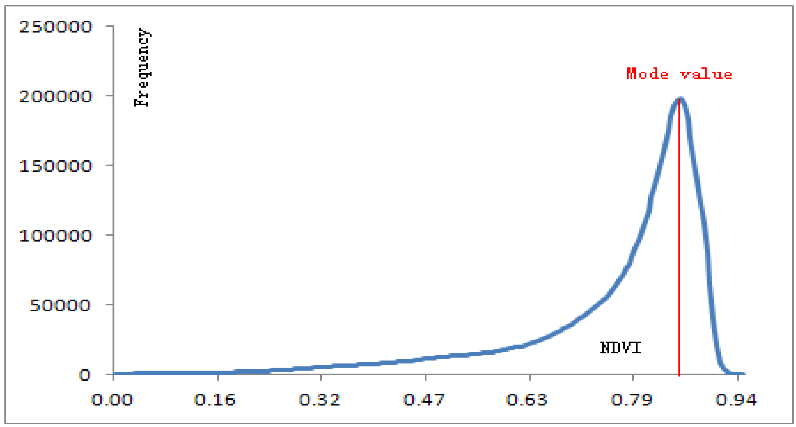
Combine the MODIS forestland data and NDVI data to obtain NDVI time characteristic curves of these three forestland categories. Combine one type of forestland with NDVI data of a certain phase and calculate the largest-frequency NDVI value as the NDVI characteristic value of the given type of forestland at a given time point (Figure 1), get the NDVI mode value of the 23 annual time phases, and draw NDVI mode curves of the forestland.
(iii)
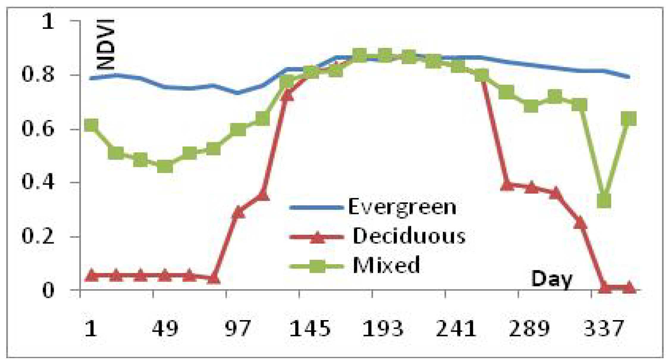
Calculate the NDVI distribution interval of each type of forestland in each phase (Figure 2). After the combination of forestland and NDVI data, the next step is to calculate the standard deviation of the forestland NDVI data and then use the NDVI characteristic value as the center value and a standard deviation above and below this value as the wave range to calculate the forestland NDVI distribution interval in a certain time phase.
Figure 1. Normalized Difference Vegetation Index (NDVI) mode value calculation.
Forests 04 00632 g001
Figure 2. Forestland NDVI histogram curve and mode value.
Forests 04 00632 g002
Normal distribution is an ideal assumption for a kind of vegetation NDVI histogram. Of course in reality, this is not the case. The reason could be that the assumption is not accurate, or the forest land classification is not completely correct. If a data distribution is approximately normal then about 68% of the data values are within one standard deviation of the mean. An interval of [mode − one standard deviation, mode + one standard deviation] is used to limit specific vegetation. The largest value of mode + one standard deviation is not more than 1.0. And we found that under the criteria, we could identify most vegetation. So being the only results so far, the mode with a standard deviation is used in this paper.

2.3.1. Forestland NDVI Characteristic Curve Calculation

There are usually four typical points, representing four transition dates [47]: (i) Greenup, the date of onset of photosynthetic activity; (ii) Maturity, the date at which the plant green leaf area is largest; (iii) Senescence, the date at which photosynthetic activity and green leaf area begin to rapidly decrease; and (iv) Dormancy, the date at which physiological activity reaches nearly zero. Relative to the other vegetation types shown in Figure 2, the NDVI values for deciduous forest (i) are higher from maturity to senescence; (ii) are lower before the greenup and after dormancy; (iii) increase rapidly from greenup to maturity. The onset of different stages during the growing season can be determined using the deciduous forest histogram mode curves: The greenup point is on the 97th day, the maturity point is on the 129th day, the senescence point is on the 257th day, and the dormancy point is on the 263th day. The main difference between deciduous and mixed forest is that the NDVI value of the latter is higher at the greenup point. The characteristics of evergreen forest are fairly obvious: The NDVI value is perennially high, with small-scale fluctuation. The mixed forestland NDVI time curve combines the characteristics of both deciduous forest and evergreen forest: The NDVI value is intermediate between evergreen forest and deciduous forest before greenup and after dormancy; it is higher than the values for the other types from maturity to senescence; and has an intermediate fluctuation range throughout the year.

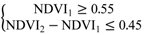
2.3.2. Evergreen Forest Estimation

The threshold to estimate evergreen forest can be determined using time series NDVI histogram mode values of evergreen forestland as a reference and one standard deviation as the NDVI distribution interval. According to the forest NDVI mode curve, we can identify the four transition points at which the change rate of curvature is largest during the growing season: Greenup on the 97th day, maturity on the 129th day, senescence on the 257th day, and dormancy on the 263th day. The threshold is determined by the NDVI histogram mode curve characteristic value and standard deviation in the given period. The specific calculation process is as follows.
From the first day to the 81st day, the mean evergreen forestland NDVI value is 0.78, the standard deviation is 0.23, the NDVI1 distribution interval is [0.55, 1] (upper limit of 1). Similarly, from the 145th day to 241st day, the NDVI2 distribution interval is [0.63, 1]. When calculating ΔNDVI, assign the lower limit to NDVI1 and the upper limit to NDVI2 to obtain the value of ΔNDVImax which is 0.45 in this case. To eliminate the influence of non-forestland and non-vegetation land, the criteria for evergreen forest classification should include the condition that the NDVI1 value should be no less than 0.55. To estimate evergreen forestland, we designed the following algorithm:
Forests 04 00632 i001
where NDVI1 represents the mean NDVI value of the period before the greenup point and NDVI2 represents the mean NDVI value of the period from maturity to senescence.

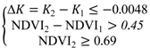
2.3.3. Deciduous Forest Estimation

The key to deciduous forestland classification is distinguishing it from single crops. From Figure 3, which shows the NDVI mode curves of single crops and deciduous forestland, we can see that the changes in the NDVI mode curves with time are similar with some important differences.
Figure 3. Time series NDVI mode curves of single crops and deciduous forest.
Forests 04 00632 g003
The main differences lie in starting point and rate of change (curve slope) as the NDVI value increases. Moreover, the valley-peak curve shape is also different. The starting point from which the deciduous forestland NDVI value grows rapidly is the 113th day, whereas that of the single crops is the 161st day. Their NDVI values increase at different rates, and on approximately the 225th day, the NDVI curve begins to turn down. Therefore, to distinguish deciduous forestland from single crops, we chose the NDVI time curve of two periods as a research object: From the 97th day to the 161st day and from the 161st day to the 225th day.
In addition to a ΔNDVImax value, which is defined as the max value of NDVI2−NDVI1, greater than 0.45, the mean NDVI of the period from the 145th day to 241st should be no less than the lower limit of the distribution interval of NDVI2 in the period from the 145th day to the 241th. Namely, deciduous forestland should meet the following conditions: ΔNDVI should be larger than 0.45 and NDVI2 should be no less than 0.69. Thus, to estimate deciduous forest, we have the following algorithm:
Forests 04 00632 i002
where K2 is the average slope (x axis for days, y axis for NDVI value) of the NDVI mode curve in the second period and K1 is the average slope in the first period. From the existing time series curves, we can see that the single crop NDVI value increases in the second period; theoretically, ∆K should be greater than zero. However, in practice, there may be some uncertainties in the NDVI observations. Thus, the calculation of the threshold of ∆K is still based on the statistics of the NDVI mode values, and the threshold is −0.0048.

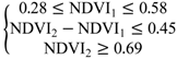
2.3.4. Mixed Forest Estimation

Mixed forestland combines the characteristics of deciduous and evergreen forestland; thus, its NDVI distribution characteristics are intermediate to those of deciduous and evergreen forestland. Specifically, the NDVI mode values differ somewhat between summer and winter, the winter NDVI values are intermediate between deciduous and evergreen forestland, and the NDVI values are higher in summer. Thus, the mixed forestland NDVI value should meet the following conditions: NDVI1 is in the interval of [0.28, 0.55], ΔNDVI is no larger than 0.45, and NDVI2 is no less than 0.69.
Forests 04 00632 i003
Due to the absence of a detailed, clear, NDVI-based classification definition for mixed forestland, some error may exist in the classification of these three types of forestland, but the overall forestland information is accurate.

2.4. Validation Approach

To provide a quantitative assessment of the accuracy of the forests distribution obtained in this paper, we performed a validation analysis using the GlobCover land use data.
The GlobCover land use data produced by the European Space Agency (ESA) are remote sensing image classification data from the ENVISAT MERIS sensor with a 300-m × 300-m spatial resolution. The updated data are for years 2005–2006, and 2009, including two images. With a nominal pixel size of 300-m × 300-m, GlobCover represents the highest spatial resolution global land cover dataset currently available [29]. The overall accuracy of GlobCover data weighted by the class area reaches 67.5% [48] and 73% [49]. The results from a cross-validation analysis indicate that the overall accuracy of MODIS LC-1 product is about 75% [13]. The agreement between GlobCover, MODIS LC-1 and other two land cover products is between 56% and 69% [18]. The accuracy of Globcover is close to that of MODIS LC-1. Therefore, to a certain extent, we can use GlobCover data to check the new results by comparing whether there are big differences between them and MODIS LC-1 data.
The new forests results were evaluated using independent validation samples disjoint from the 2009 image. The validated samples were extracted from GlobCover in a strict standard. They were selected using a random probability sampling scheme. The deciduous forest was evaluated using the closed (tree cover >40%) broadleaf deciduous forest (tree height >5 m) in GlobCover. The evergreen forest was evaluated using the closed (tree cover >40%) needleleaf evergreen forest (tree height >5 m). The mixed forest was evaluated using the closed to open (tree cover >15%) mixed broadleaf and needleleaf forest (tree height >5 m). In order to improve the accuracy of validated points, the mean NDVI value of the period from maturity to senescence should be larger than 0.5. This assessment considers rather homogeneous samples and computes common accuracies derived from the error matrix, producer’s, user’s, and overall accuracy [50].
The definitions used in this paper of the different forest types are the same as MODIS LC-1. As the first results, we merged five different types of forests in MODIS LC-1 into three broader categories: deciduous forests, evergreen forests, and mixed forests. The definitions of different forest types were listed in the Table 2.
Table 2. The definitions of different forest types.
This paperMODIS LC-1Validated with GlobCover
deciduous forestsDeciduous Needleleaf Forestsclosed (tree cover >40%) broadleaf deciduous forest (tree height >5 m)
Deciduous Broadleaf Forests
evergreen forestsEvergreen Needleleaf Forestsclosed (tree cover >40%) needleleaf evergreen forest (tree height >5 m)
Evergreen Broadleaf Forests
mixed forestsmixed forestsclosed to open (tree cover >15%) mixed broadleaf and needleleaf forest (tree height >5 m)

3. Results and Discussion

3.1. Comparison and Validation

The forest coverage for 2001 to 2011 was estimated from the MODIS NDVI time series data based on the histogram method. To compare the differences between new results and MODIS forest type, as an example, the two data in 2007 were selected to compare. The 2009 new forest data was then validated with ESA GlobCover.
Relative to the MODIS data, the amount of forestland pixels got with the histogram method is also improved. According to the statistics, the forestland pixels in MODIS only account for approximately 15% of the total pixels; however, the actual total forest coverage over China is 18.21% in 2003 [51] and 20.36% in 2008 [52]. The total percentage of forestland pixels in MODIS LC-1 classification data are underestimated. Although the differences in percentage are small, the differences in pixels number are huge. These results will be more reasonable if the percentage is larger than the true value since most pixels are generally mixed pixels in the middle-resolution remotely sensed images.
The forestland pixels acquired based on the new method account for approximately 31% of the total pixels, which is higher than the national forest coverage in 2008. The reason for this difference is the existence of mixed pixels in the remote sensing images. This result also shows that the forestland data estimated from middle-resolution images can only represent the geographical distribution of forestland; further research is being carried out on the estimation of forest area.
The Comparison of 2001 forest distribution is shown in Figure 4. Green (Unchanged) indicates that both data sets classify this land as forest. Blue (Increased) indicates that the area is classified as forest in the histogram results but not in MODIS. Red (Decreased) indicates that the area is classified as forest in the MODIS landcover data but not in the histogram results. Neither of them is forest in the white area. To analyze the differences between these two types of data, relevant investigations, including Google Earth, thematic maps of all vegetation types, and forest investigation data, have been verified. For example, the new results are forests now, while they are not forests in MODIS LC-1 at the junction areas of Sichuan and Chongqing. The new results were validated through Google earth. Most areas in the Northeast of China are forestland, the same as thematic maps but are classified as crop in MODIS LC-1. The result shows that the newly estimated forestland data is superior to the forestland data in MODIS. The missed or misclassified MODIS forestland pixels are re-classified correctly in this study.
Using more than ten thousand samples of forestland data from ESA GlobCover as a reference, the estimation accuracies of the newly estimated forestland information and MODIS forestland information are calculated. This process includes the calculation of the producer’s accuracy of forestland classification and the user’s accuracy.
Figure 4. Forest distribution of China in 2001. Green (Unchanged) indicates that both data sets classify this land as forest. Blue (Increased) indicates that the area is classified as forest in the histogram results but not in MODIS. Red (Decreased) indicates that the area is classified as forest in the MODIS landcover data but not in the histogram results.
Forests 04 00632 g004
From the Table 3, we can see that the overall accuracy of the newly classified data is 0.128 higher than that of the MODIS surface classification data. Thus, the time-series-based classification method can indeed improve the accuracy of forestland estimation. In contrast, many forestland pixels are missed in MODIS data.
Table 3. Accuracy of validation.
TypesProducer’s accuracyUser’s accuracyOverall accuracy
This paperDeciduous 0.895 0.994 0.804
Evergreen 0.940 0.793
Mixed 0.600 0.936
MODISDeciduous 0.651 0.722 0.676
Evergreen 0.673 0.987
Mixed 0.701 0.625

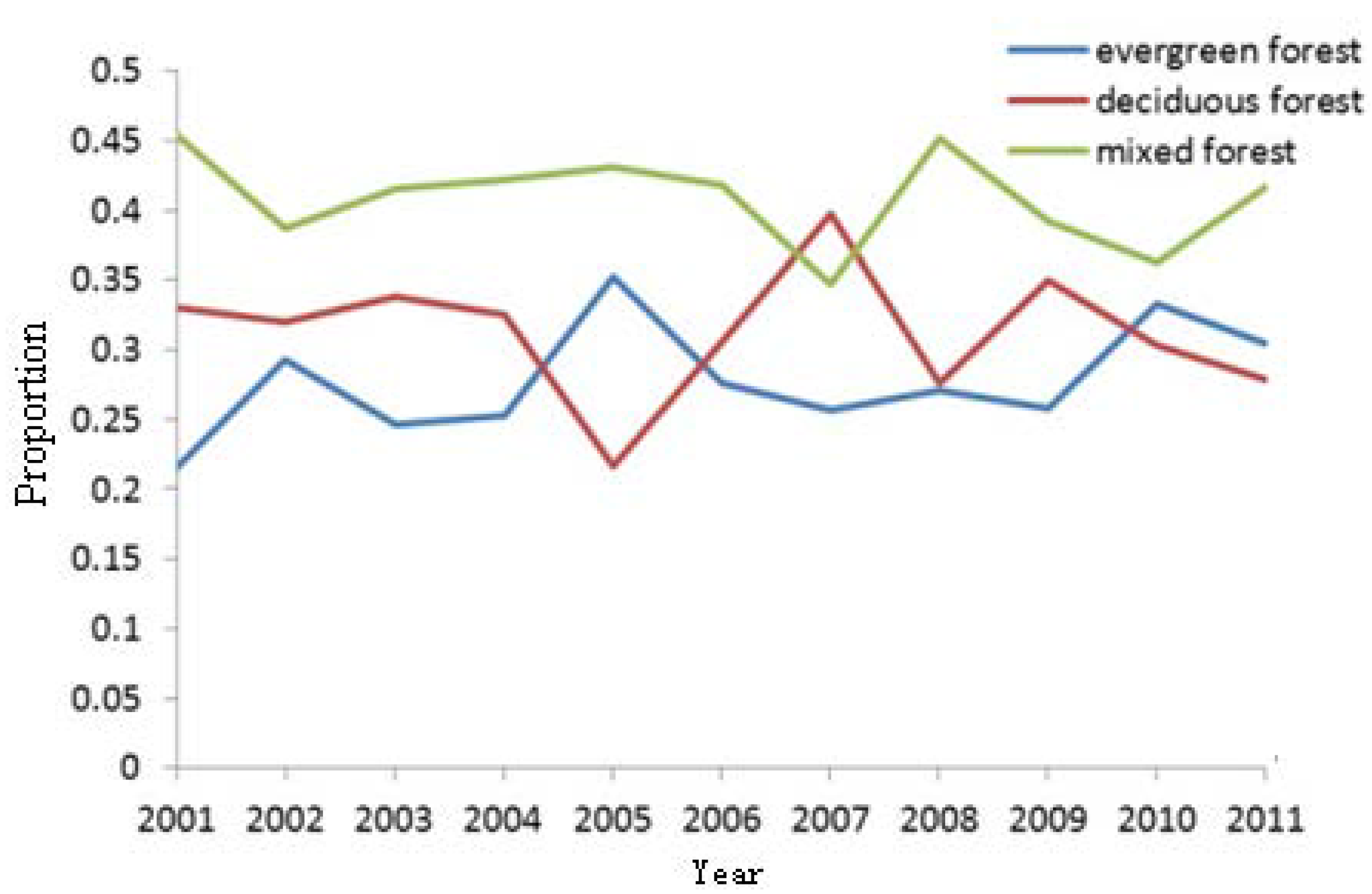
3.2. China Forestland Analysis, 2001–2011

Based on the method above, we prepared the forestland distribution charts for 2001–2011. China has rich forest resources, and the distribution of forestland clearly exhibits regional variation. From a national perspective, the forestland pixels and mixed forestland pixels over the past 11 years accounted for an average of 33.72% of all pixels. The respective proportion for each year and the fitted curve are shown in Figure 5. The linear fitting model of the proportion of forestland pixels is =0.1195X-205.98, and the slope coefficient k is 0.1195, which indicates that there is a gradual increase in China’s forestland coverage during 2001–2011. Tests of significance have been done and p value is 0.399, so the relationship is not statistically significant.
Figure 5. Forest coverage changes in China over the past 11 years.
Forests 04 00632 g005
The results show that among the three types of forestland, the distribution area of mixed forestland is the largest. In 2001–2011, the pixels of mixed forestland account for an average of 40.91% of the total forestland pixels. For the other two types of forestland, the distribution of the evergreen forestland (31.28%) is slightly higher than that of the deciduous forest (27.81%). The proportion changes of the three types of forestland with time are shown in Figure 6. The proportion of all three types of forestland changed dramatically during 2005–2007 because of logging and regeneration. The forests in south China are mainly evergreen and mixed forests, of which the evergreen forest is concentrated in southern Tibet, Yunnan, and southeastern regions. The deciduous and mixed forests are mainly distributed in northern China, of which most are in Heilongjiang, Liaoning, and Jilin and a small amount is in the Tianshan area in Xinjiang.
Figure 6. Proportion changes of three categories of forestland over the past 11 years.
Forests 04 00632 g006
In addition, this paper also analyzes the forestland pixel proportion of each province and conducts a linear fitting of the proportion and time trends. The slope of the line represents the forestland proportion changes: If positive, the proportion of forestland is increasing; if negative, the proportion is decreasing. Figure 7 presents the regional distribution of the newly emerging forestland in China during 2001–2011, from which we can see that the increase during these 11 years is mainly located in central China and three northern areas of China. The range of China’s forestland coverage has expanded over the past 11 years, but the extent of the increase varies by province. The increasing trends in Beijing, Henan, and Hebei are apparent and higher than the national average level; on the other extreme, the forestland coverages of Shanghai and Jiangsu are decreasing and far below the national level.
Figure 7. Forestland variation tendency over the past 11 years.
Forests 04 00632 g007

3.3. Uncertainty Analysis

The uncertainty of the forestland information estimation in this paper is associated with the following aspects:
(i)
The surface classification systems are different among different products, such as the MODIS and MERIS GlobCover data, since they are produced using varied methods [14,15,16,18]. Therefore, validation errors may be introduced in the merging of forestland information.
(ii)
Disease and pests, forest fires, weather, and other factors may also affect the remote-sensing observation of NDVI and thereby the forest NDVI values as well as the final estimation results. This paper has discussed the effect of weather on NDVI value. However, it will be difficult to use disease and pests as well as fire disasters as variables to constrain the estimation of forest information. Further studies are required on the effect of disease, pests, and fire disasters on NDVI value and their constraints on forestland information estimation.
(iii)
Relative to the existing land use data and forest investigation data, the forestland pixel area obtained in this paper is larger due to the consideration of mixed pixels. In the classification of medium- and low-resolution remotely sensed images, if the forestland area comprises a certain percentage of a pixel, the pixel will be classified as forestland. This approach is different from that used in the land use survey data and the forest investigation data. Hence, this paper estimated only the location information of the forestland, and further studies on the specific coverage area are needed. In addition, the overall regional distribution of forestland in China will not be affected.

4. Conclusions

Forests provide resources and environmental conditions on which humans rely for existence. In this work, a methodology for the estimation of forest types is proposed. The new algorithm is based on the combination of MODIS NDVI with a classification of the land surface (MODIS LC-1). The new method can be used to estimate forest cover information and can improve classification accuracy. The main conclusions from the forestland information estimation consist of the following points:
(i)
The histogram mode feature of forestland and a decision tree classification method can be used to estimate the forest cover information and can improve its classification accuracy. The forestland data for China over the past 11 years are acquired using the NDVI time series histogram mode characteristics. The spatial distribution of the forest over China is more consistent with reality than that in MCD12Q1. The obtained data can more accurately reflect the actual conditions of the forestland in China and may effectively improve the overall accuracy for forestland compared with the existing MODIS surface classification data.
(ii)
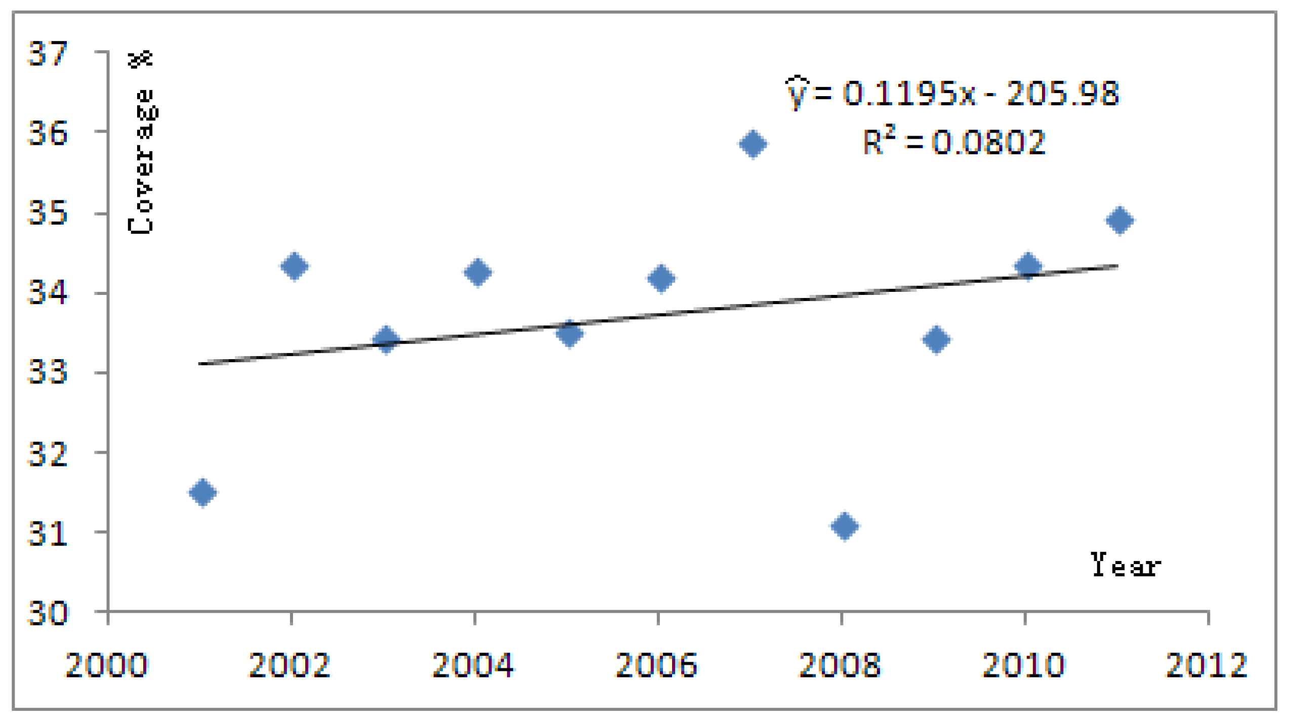
Based on the results of estimated forestland, the forestland pixels in China over the past 11 years account for an average of 33.72% of the total pixels of inland areas. Differentiation and variation are observed in the spatial distributions of forestland. Forestland is mainly found in southern China, northeastern China, southern Tibet, and the Tianshan (Xinjiang) area. The evergreen forestland is concentrated in southern Tibet, Yunnan, and southeastern China; and the deciduous forestland is distributed in northern China, mostly in the northeast. The forestland coverage of northwestern China is relatively small, such as in Qinghai and Gansu.
(iii)
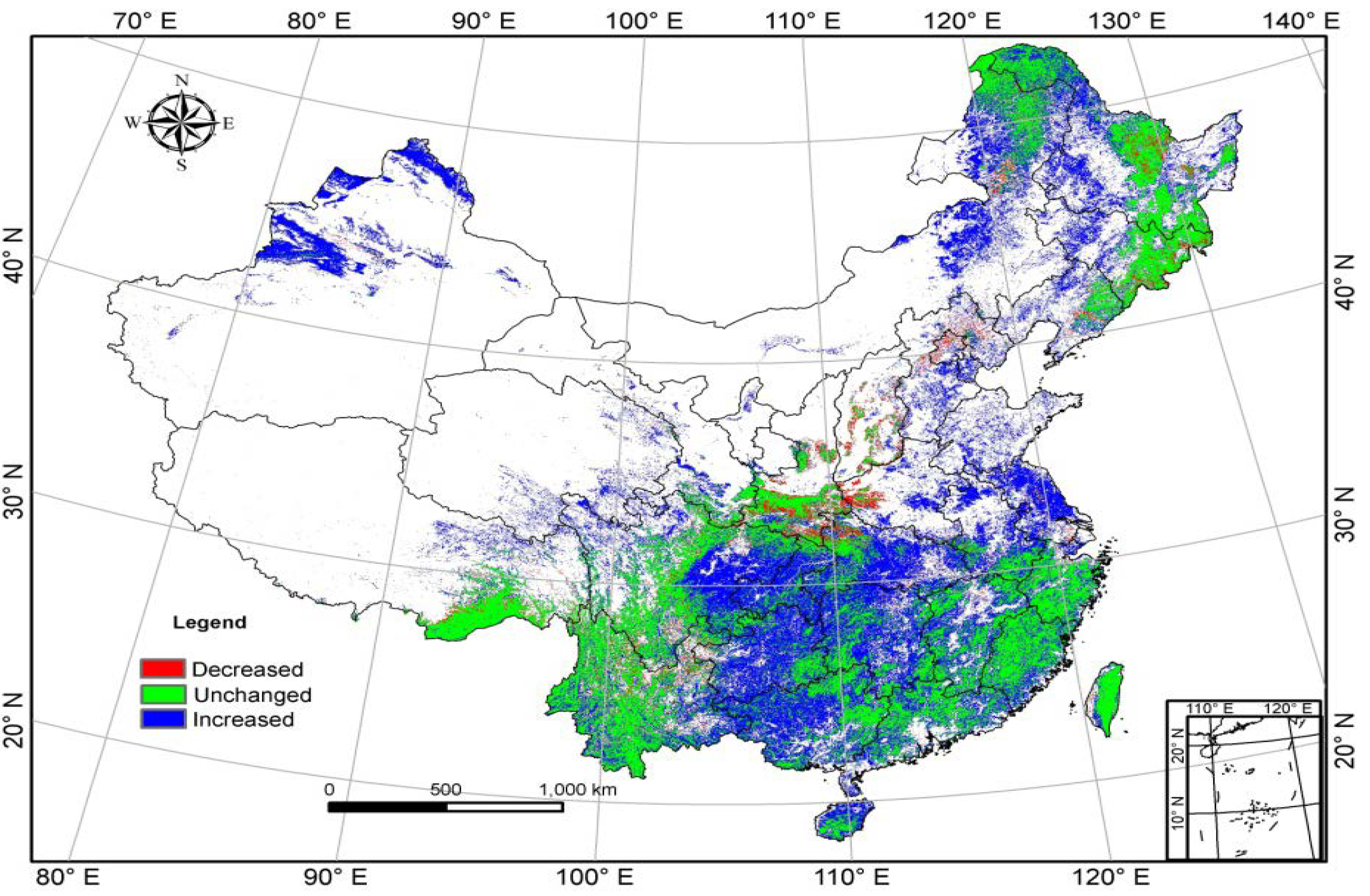
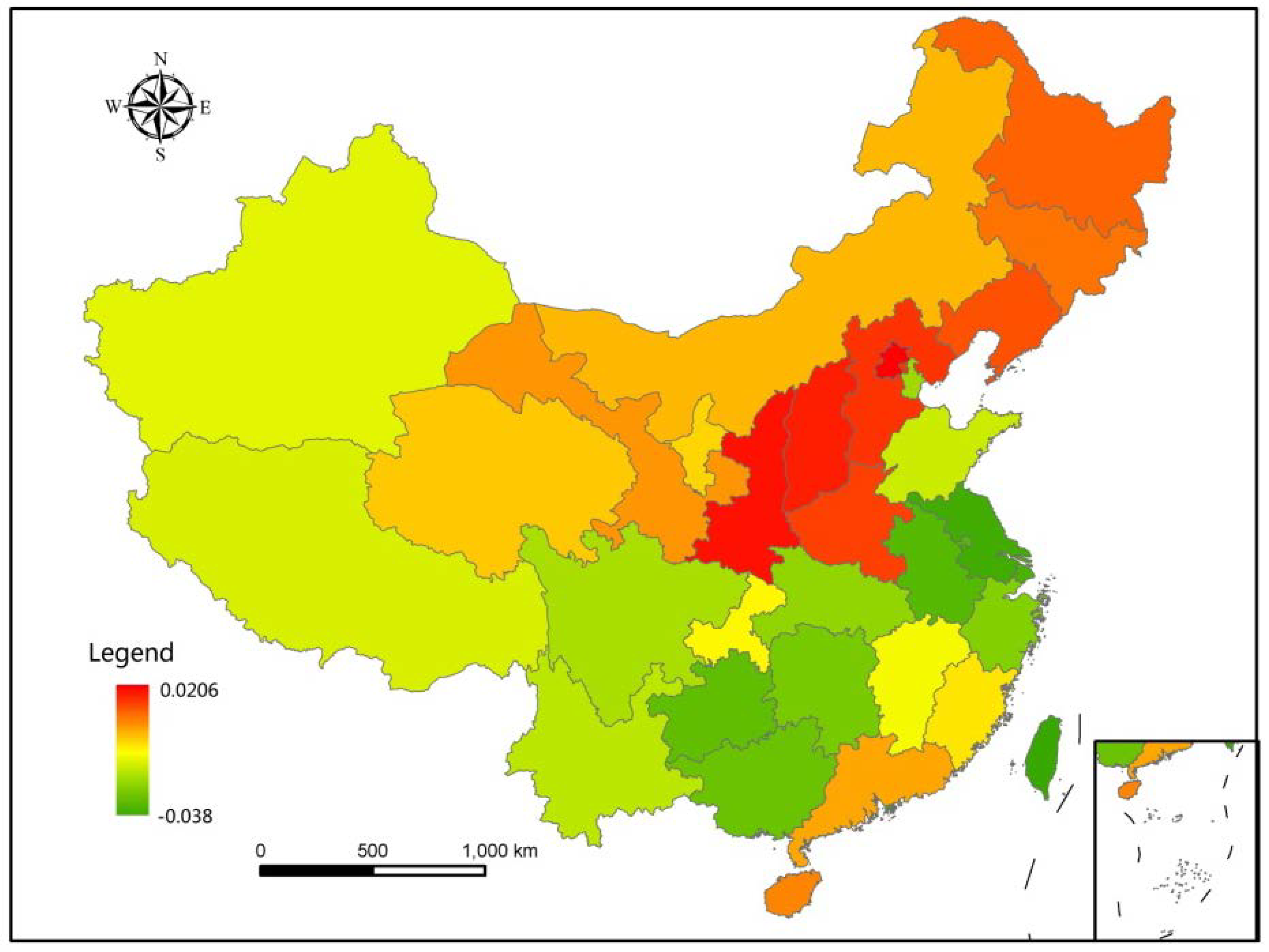
In the past 11 years, the changes of each province’s forestland coverage range differ somewhat but increased overall, with central China and three northern areas of China having the largest increases. Over the past 11 years, evergreen forestland pixels have accounted for an average of 31.28% of the total forestland pixels. Deciduous and mixed forestlands are scattered across the country but are fairly concentrated in the temperate zone located in central China, accounting for an average of 27.81% and 40.91% of total forestland, respectively.
(iv)
Of the forestland data estimated in this paper, all the forestland pixels are mixed pixels, and certain differences do exist between the forestland distribution range and the actual area of the forestland. Besides this, the equations used to calculate forest cover would vary from region to region, and would require different thresholds or time intervals based on the variables of latitude/longitude. Further studies need to analyze the differences among different locations to develop different thresholds. In addition, the research method applied in this paper will also be applied in the estimation for other surface features, such as crop and grassland estimation.

Acknowledgments

This research was supported by National Basic Research Program of China (2012CB955401) and the project of State Key Laboratory of Earth Surface Processes and Resource Ecology (2011-KF-08). The authors wish to thank the anonymous referees for their valuable comments. The authors also acknowledge the ESA GlobCover project for the provision of GlobCover data.

Conflict of Interest

The authors declare no conflict of interest.

References

  1. Food and Agriculture Organization (FAO), State of the World’s Forests 2012. Food and Agriculture Organization of the United Nations: Rome, Italy, 2012.
  2. Bonan, G.B. Forests and climate change: Forcings, feedbacks, and the climate benefits of forest. Science 2008, 320, 1444–1449. [Google Scholar] [CrossRef]
  3. Curran, L.M.; Trigg, S.N.; McDonald, A.K.; Astiani, D.; Hardiono, Y.M.; Siregar, P.; Caniago, I.; Kasischke, E. Lowland forest loss in protected areas of indonesian borneo. Science 2004, 303, 1000–1003. [Google Scholar] [CrossRef]
  4. Gorsevski, V.; Kasischke, E.; Dempewolf, J.; Loboda, T.; Grossmann, F. Analysis of the impacts of armed conflict on the Eastern Afromontane forest region on the South Sudan-Uganda border using multitemporal Landsat imagery. Remote Sens. Environ. 2012, 118, 10–20. [Google Scholar] [CrossRef]
  5. Achard, F.; Eva, H.D.; Stibig, H.-J.; Mayaux, P.; Gallego, J.; Richards, T.; Malingreau, J.-P. Determination of deforestation rates of the World’s humid tropical forests. Science 2002, 297, 999–1002. [Google Scholar] [CrossRef]
  6. Verbesselt, J.; Robinson, A.; Stone, C.; Culvenor, D. Forecasting tree mortality using change metrics derived from MODIS satellite data. For. Ecol. Manag. 2009, 258, 1166–1173. [Google Scholar] [CrossRef]
  7. Hansen, M.C.; Roy, D.P.; Lindquist, E.; Adusei, B.; Justice, C.O.; Altstatt, A. A method for integrating MODIS and Landsat data for systematic monitoring of forest cover and change in the Congo Basin. Remote Sens. Environ. 2008, 112, 2495–2513. [Google Scholar] [CrossRef]
  8. Loveland, T.R.; Reed, B.C.; Brown, J.F.; Ohlen, D.O.; Zhu, Z.; Yang, L.; Merchant, J.W. Development of a global land cover characteristics database and IGBP DISCover from 1 km AVHRR data. Int. J. Remote Sens. 2000, 21, 1303–1330. [Google Scholar] [CrossRef]
  9. Hansen, M.C.; Defries, R.S.; Townshend, J.R.G.; Sohlberg, R. Global land cover classification at 1 km spatial resolution using a classification tree approach. Int. J. Remote Sens. 2000, 21, 1331–1364. [Google Scholar] [CrossRef]
  10. Hansen, M.C.; Reed, B. A comparison of the IGBP DISCover and University of Maryland 1 km global land cover products. Int. J. Remote Sens. 2000, 21, 1365–1373. [Google Scholar] [CrossRef]
  11. Bartholomé, E.; Belward, A.S. GLC2000: A new approach to global land cover mapping from Earth observation data. Int. J. Remote Sens. 2005, 26, 1959–1977. [Google Scholar] [CrossRef]
  12. Friedl, M.A.; McIver, D.K.; Hodges, J.C.F.; Zhang, X.Y.; Muchoney, D.; Strahler, A.H.; Woodcock, C.E.; Gopal, S.; Schneider, A.; Cooper, A.; et al. Global land cover mapping from MODIS: Algorithms and early results. Remote Sens. Environ. 2002, 83, 287–302. [Google Scholar] [CrossRef]
  13. Friedl, M.A.; Sulla-Menashe, D.; Tan, B.; Schneider, A.; Ramankutty, N.; Sibley, A.; Huang, X. MODIS Collection 5 global land cover: Algorithm refinements and characterization of new datasets. Remote Sens. Environ. 2010, 114, 168–182. [Google Scholar] [CrossRef]
  14. Arino, O.; Gross, D.; Ranera, F.; Bourg, L.; Leroy, M.; Bicheron, P.; Latham, J.; di Gregorio, A.; Brockman, C.; Witt, R.; et al. GlobCover: ESA Service for Global Land Cover from MERIS. In Proceedings of IEEE International Geoscience and Remote Sensing SymposiumIGARSS 2007, Barcelona, Spain, 23–28 July 2007; pp. 2412–2415.
  15. Defourny, P.; Vancutsem, C.; Bicheron, P.; Brockmann, C.; Nino, F.; Schouten, L.; Leroy, M. GLOBCOVER: A 300 m Global Land Cover Product for 2005 Using Envisat MERIS Time Series. In Proceedings of the ISPRS Commission VII Mid-Term SymposiumRemote Sensing: From Pixels to Processes, Enschede, The Netherlands, 8–11 May 2006; pp. 8–11.
  16. Yaqian, H.; Yanchen, B. A Consistency Analysis of MODIS MCD12Q1 and MERIS Globcover Land Cover Datasets over China. In Proceedings of 19th International Conference on Geoinformatics, Shanghai, China, 24–26 June 2011; pp. 1–6.
  17. Stehman, S.V.; Olofsson, P.; Woodcock, C.E.; Herold, M.; Friedl, M.A. A global land-cover validation data set, II: Augmenting a stratified sampling design to estimate accuracy by region and land-cover class. Int. J. Remote Sens. 2012, 33, 6975–6993. [Google Scholar] [CrossRef]
  18. Kaptué Tchuenté, A.T.; Roujean, J.-L.; de Jong, S.M. Comparison and relative quality assessment of the GLC2000, GLOBCOVER, MODIS and ECOCLIMAP land cover data sets at the African continental scal. Int. J. Appl. Earth Obs. Geoinf. 2011, 13, 207–219. [Google Scholar] [CrossRef]
  19. Herold, M.; Mayaux, P.; Woodcock, C.E.; Baccini, A.; Schmullius, C. Some challenges in global land cover mapping: An assessment of agreement and accuracy in existing 1 km datasets. Remote Sens. Environ. 2008, 112, 2538–2556. [Google Scholar] [CrossRef]
  20. Zhao, X.; Liang, S.; Liu, S.; Yuan, W.; Xiao, Z.; Liu, Q.; Cheng, J.; Zhang, X.; Tang, H.; Zhang, X.; et al. The Global Land Surface Satellite (GLASS) remote sensing data processing system and products. Remote Sens. 2013, 5, 2436–2450. [Google Scholar] [CrossRef]
  21. Liang, S.; Zhao, X.; Yuan, W.; Liu, S.; Cheng, X. A long-term Global Land Surface Satellite (GLASS) dataset for environmental studies. Int. J. Digit. Earth 2013, in press. [Google Scholar]
  22. Kennedy, R.E.; Cohen, W.B.; Schroeder, T.A. Trajectory-based change detection for automated characterization of forest disturbance dynamics. Remote Sens. Environ. 2007, 110, 370–386. [Google Scholar] [CrossRef]
  23. Kennedy, R.E.; Yang, Z.; Cohen, W.B. Detecting trends in forest disturbance and recovery using yearly Landsat time series: 1. LandTrendr-Temporal segmentation algorithms. Remote Sens. Environ. 2010, 114, 2897–2910. [Google Scholar] [CrossRef]
  24. Cohen, W.B.; Yang, Z.; Kennedy, R. Detecting trends in forest disturbance and recovery using yearly Landsat time series: 2. TimeSync—Tools for calibration and validation. Remote Sens. Environ. 2010, 114, 2911–2924. [Google Scholar] [CrossRef]
  25. Griffiths, P.; Kuemmerle, T.; Kennedy, R.E.; Abrudan, I.V.; Knorn, J.; Hostert, P. Using annual time-series of Landsat images to assess the effects of forest restitution in post-socialist Romania. Remote Sens. Environ. 2012, 118, 199–214. [Google Scholar] [CrossRef]
  26. Kennedy, R.E.; Townsend, P.A.; Gross, J.E.; Cohen, W.B.; Bolstad, P.; Wang, Y.Q.; Adams, P. Remote sensing change detection tools for natural resource managers: Understanding concepts and tradeoffs in the design of landscape monitoring projects. Remote Sens. Environ. 2009, 113, 1382–1396. [Google Scholar] [CrossRef]
  27. Kennedy, R.E.; Yang, Z.; Cohen, W.B.; Pfaff, E.; Braaten, J.; Nelson, P. Spatial and temporal patterns of forest disturbance and regrowth within the area of the Northwest Forest Plan. Remote Sens. Environ. 2012, 122, 117–133. [Google Scholar] [CrossRef]
  28. Pflugmacher, D.; Cohen, W.B.; Kennedy, E.R. Using Landsat-derived disturbance history (1972–2010) to predict current forest structure. Remote Sens. Environ. 2012, 122, 146–165. [Google Scholar] [CrossRef]
  29. Pflugmacher, D.; Krankina, O.N.; Cohen, W.B.; Friedl, M.A.; Sulla-Menashe, D.; Kennedy, R.E.; Nelson, P.; Loboda, T.V.; Kuemmerle, T.; Dyukarev, E.; et al. Comparison and assessment of coarse resolution land cover maps for Northern Eurasia. Remote Sens. Environ. 2011, 115, 3539–3553. [Google Scholar] [CrossRef]
  30. Meigs, G.W.; Kennedy, R.E.; Cohen, W.B. A Landsat time series approach to characterize bark beetle and defoliator impacts on tree mortality and surface fuels in conifer forests. Remote Sens. Environ. 2011, 115, 3707–3718. [Google Scholar] [CrossRef]
  31. Zhu, Z.; Woodcock, C.E.; Olofsson, P. Continuous monitoring of forest disturbance using all available Landsat imagery. Remote Sens. Environ. 2012, 122, 75–91. [Google Scholar] [CrossRef]
  32. Xin, Q.; Olofsson, P.; Zhu, Z.; Tan, B.; Woodcock, C.E. Toward near real-time monitoring of forest disturbance by fusion of MODIS and Landsat data. Remote Sens. Environ. 2013, 135, 234–247. [Google Scholar] [CrossRef]
  33. Rodriguez-Galiano, V.F.; Chica-Olmo, M.; Abarca-Hernandez, F.; Atkinson, P.M.; Jeganathan, C. Random Forest classification of Mediterranean land cover using multi-seasonal imagery and multi-seasonal texture. Remote Sens. Environ. 2012, 121, 93–107. [Google Scholar] [CrossRef]
  34. Schapire, R.E.; Freund, Y.; Bartlett, P.L.; Lee, W.S. Boosting the margin: A new explanation for the effectiveness of voting methods. Ann. Stat. 1998, 26, 1651–1686. [Google Scholar] [CrossRef]
  35. Huete, A.; Didan, K.; Miura, T.; Rodriguez, E.P.; Gao, X.; Ferreira, L.G. Overview of the radiometric and biophysical performance of the MODIS vegetation indices. Remote Sens. Environ. 2002, 83, 195–213. [Google Scholar] [CrossRef]
  36. Loveland, T.R.; Belward, A.S. The IGBP-DIS global 1 km land cover data set, DISCover: First results. Int. J. Remote Sens. 1997, 18, 3289–3295. [Google Scholar] [CrossRef]
  37. Lotsch, A.; Tian, Y.; Friedl, M.A.; Myneni, R.B. Land cover mapping in support of LAI and FPAR retrievals from EOS-MODIS and MISR: Classification methods and sensitivities to errors. Int. J. Remote Sens. 2003, 24, 1997–2016. [Google Scholar] [CrossRef]
  38. Myneni, R.B.; Hoffman, S.; Knyazikhin, Y.; Privette, J.L.; Glassy, J.; Tian, Y.; Wang, Y.; Song, X.; Zhang, Y.; Smith, G.R.; et al. Global products of vegetation leaf area and fraction absorbed PAR from year one of MODIS data. Remote Sens. Environ. 2002, 83, 214–231. [Google Scholar] [CrossRef]
  39. Running, S.W.; Loveland, T.R.; Pierce, L.L.; Nemani, R.R.; Hunt, E.R., Jr. A remote sensing based vegetation classification logic for global land cover analysis. Remote Sens. Environ. 1995, 51, 39–48. [Google Scholar] [CrossRef]
  40. Bonan, G.B.; Levis, S.; Kergoat, L.; Oleson, K.W. Landscapes as patches of plant functional types: An integrating concept for climate and ecosystem models. Glob. Biogeochem. Cycles 2002, 16, 1–23. [Google Scholar] [CrossRef]
  41. Justice, C.O.; Townshend, J.R.G.; Vermote, E.F.; Masuoka, E.; Wolfe, R.E.; Saleous, N.; Roy, D.P.; Morisette, J.T. An overview of MODIS Land data processing and product status. Remote Sens. Environ. 2002, 83, 3–15. [Google Scholar] [CrossRef]
  42. Omuto, C.T. A new approach for using time-series remote-sensing images to detect changes in vegetation cover and composition in drylands: A case study of eastern Kenya. Int. J. Remote Sens. 2011, 32, 6025–6045. [Google Scholar] [CrossRef]
  43. Pan, Y.; Li, L.; Zhang, J.; Liang, S.; Zhu, X.; Sulla-Menashe, D. Winter wheat area estimation from MODIS-EVI time series data using the Crop Proportion Phenology Index. Remote Sens. Environ. 2012, 119, 232–242. [Google Scholar] [CrossRef]
  44. Sakamoto, T.; Wardlow, B.D.; Gitelson, A.A.; Verma, S.B.; Suyker, A.E.; Arkebauer, T.J. A two-step filtering approach for detecting maize and soybean phenology with time-series MODIS data. Remote Sens. Environ. 2010, 114, 2146–2159. [Google Scholar] [CrossRef]
  45. Schowengerdt, R.A. Remote Sensing: Models and Methods for Image Processing, 3rd ed.; Academic Press: Burlington, MA, USA, 2007; pp. 144–145. [Google Scholar]
  46. ENVI Reference Guide Version 4.7 August, 2009 Edition. ITT Visual Information Solutions. Available online: http://www.exelisvis.com/portals/0/pdfs/envi/Reference_Guide.pdf (accessed on 26 May 2013).
  47. Zhang, X.; Friedl, M.A.; Schaaf, C.B.; Strahler, A.H.; Hodges, J.C.F.; Gao, F.; Reed, B.C.; Huete, A. Monitoring vegetation phenology using MODIS. Remote Sens. Environ. 2003, 84, 471–475. [Google Scholar]
  48. Bontemps, S.; Defourny, P.; Bogaert, E.V.; Arino, O.; Kalogirou, V.; Perez, J.R. GLOBCOVER 2009 Products Description and Validation Report; Technical Report for ESA GlobCover project: UCLouvain & ESA Team; 2011; p. 53. Available online: http://due.esrin.esa.int/globcover/LandCover2009/GLOBCOVER2009_Validation_Report_2.2.pdf. (accessed on 26 July 2013).
  49. Pierre, D.; Leon, S.; Sergey, B.; Sophie, B.; Peter, C.; Allard, D.W.; Carlos, D.B.; Bruno, G.; Chandra, G.; Valerie, G.; et al. Accuracy Assessment of a 300 m Global Land Cover Map: The GlobCover Experience. In Proceedings of the 33rd International Symposium on Remote Sensing of Environment, Stresa, Italy, 4–9 May 2009.
  50. Congalton, R.G. A review of assessing the accuracy of classifications of remotely sensed data. Remote Sens. Environ. 1991, 37, 35–46. [Google Scholar] [CrossRef]
  51. Song, C.; Zhang, Y. Forest Cover in China from 1949 to 2006. In Reforesting Landscapes; Nagendra, H., Southworth, J., Eds.; Springer Netherlands: Dordrecht, The Netherlands, 2010; Volume 10, pp. 341–356. [Google Scholar]
  52. Xu, J.C. China’s new forests aren’t as green as they seem. Nature 2011, 477, 371. [Google Scholar] [CrossRef]

