Mapping Secondary Vegetation of a Region of Deforestation Hotspot in the Brazilian Amazon: Performance Analysis of C- and L-Band SAR Data Acquired in the Rainy Season

Abstract

The re-suppression of secondary vegetation (SV) in the Brazilian Amazon for agriculture or land speculation occurs mostly in the rainy season. The use of optical images to monitor such re-suppression during the rainy season is limited because of the persistent cloud cover. This study aimed to evaluate the potential of C- and L-band SAR data acquired in the rainy season to discriminate SV in an area of new hotspot of deforestation in the municipality of Colniza, northwestern of Mato Grosso State, Brazil. This is the first time that the potential of dual-frequency SAR data was analyzed to discriminate SV, with an emphasis on data acquired during the rainy season. The L-band ALOS/PALSAR-2 and the C-band Sentinel-1 data acquired in March 2018 were processed to obtain backscattering coefficients and nine textural attributes were derived from the gray level co-occurrence matrix method (GLCM). Then, we classified the images based on the non-parametric Random Forest (RF) and Support Vector Machine (SVM) algorithms. The use of SAR textural attributes improved the discrimination capability of different LULC classes found in the study area. The results showed the best performance of ALOS/PALSAR-2 data classified by the RF algorithm to discriminate the following representative land use and land cover classes of the study area: primary forest, secondary forest, shrubby pasture, clean pasture, and bare soil, with an overall accuracy and Kappa coefficient of 84% and 0.78, respectively. The RF outperformed the SVM classifier to discriminate these five LULC classes in 14% of overall accuracy for both ALOS-2 and Sentinel-1 data sets. This study also showed that the textural attributes derived from the GLCM method are highly sensitive to the moving window size to be applied to the GLCM method. The results of this study can assist the future development of an operation system based on dual-frequency SAR data to monitor re-suppression of SV in the Brazilian Amazon or in other tropical rainforests.

1. Introduction

Regardless of global importance of tropical forests in terms of biodiversity conservation and carbon and water cycling maintenance, the Brazilian Legal Amazon is losing, on average, about 13.8 thousand km² per year of primary forest by clear-cut deforestation since 1988 [1]. The main purposes of such deforestation are beef production, crop plantation, land speculation, and the installation of hydroelectric plants, among other activities [2,3,4,5]. Some authors have pointed out the recent increase of the deforestation rate [6,7], raising from 5000 km² of clear-cut deforestation in 2014 to 13,000 km² in 2021 [1].

Some of the clear-cut deforested areas are abandoned, entering in the process of natural regrowth through secondary succession. This regrowing vegetation is known as secondary vegetation (SV) [8,9]. According to the Global Forest Resources Assessment report of 2020 [10], the world has 3.7 billion ha of SV. The TerraClass project, coordinated by the National Institute for Space Research (INPE) and the Brazilian Agricultural Research Corporation (Embrapa Agricultura Digital and Embrapa Amazônia Oriental) [11], showed that SV has increased from 10 million ha to 17 million ha in the Brazilian Legal Amazon between 2004 and 2014 [12]. The natural regeneration of forests is an effective low-cost mechanism of carbon sequestration, particularly in tropical regions [13]. Although the net carbon uptake from atmosphere is up to 20 times higher than that from old-growth forests, this tend to be neglected in most of the carbon balance studies in the Brazilian Amazon [14]. Besides its particular interest as source of carbon sink, SV can be seen as having great potential for agriculture and livestock expansion [15] or for biodiversity conservation and ecosystem service [16].

Nunes et al. [17] highlighted different aspects related to the growing pressure to suppress already-deforested SV found in the Brazilian Amazon. For example, landowners face difficulty to find ways to monetize climate change mitigation and other ecosystem services provided by SV. The Brazilian Federal Law No. 12651, known as the Brazilian Forest Code, does not protect or regulate land use in areas occupied by regenerating forests. On the other hand, the same Brazilian Forest Code places severe restrictions for deforesting native forests located in the Brazilian Amazon biome. Landowners must keep 80% of their rural properties preserved by native forests [18], encouraging the use of existing regrowing lands.

The current deforestation monitoring system of the Brazilian Amazon such as the Project of Monitoring Deforestation of the Brazilian Amazon Forest by Satellite (PRODES) [1], Near Real-Time Deforestation Detection System (DETER-B) [19], and Deforestation Alert System (SAD) [20] do not monitor SV since they track only clear-cut deforestation, selective logging, and degradation by fire that occurs in primary forests, masking previously deforested areas as well as non-forest native vegetation formations. The TerraClass Amazon project [11] is the only project aimed at monitoring secondary vegetation every two years. In this project, clear-cut deforested areas detected by the PRODES are inspected by Landsat-like satellite images (i.e., typically, 30 m spatial resolution and 16 day repeat-pass) after two years to determine the corresponding land use and land cover (LULC) class, for example, pasture, cropland, or SV. More recently, Nunes et al. [17] assessed the extent, age, net carbon balance, and annual dynamics of the SV in the Brazilian Amazon by using the LULC maps derived from Landsat time series and produced by the MapBiomas project [21] from 1985 to 2017. The SV area has increased over time, reaching 12 million ha in 2017, 44% of which was under 5 years old. Indeed, most of the estimations of the extent of the SV is often conducted based on remote sensing data derived from optical sensors e.g., [22,23].

Long time series of optical satellite data such as the Landsat historical data provide important information on the spatial and temporal patterns of deforested areas in the process of regeneration in the Brazilian Amazon. However, because of the constraints related to the persistent cloud coverage in tropical regions, optical remote-sensing-derived information of SV will be mostly related to the peak of the dry season, which is from July to September in the Brazilian Amazon. Thus, studies involving the seasonal variations of SV, similar to the one conducted by [24] in an Amazon tropical evergreen forest, or re-suppression monitoring of SV, which typically occurs during the end of the wet season, will be limited. Although the Brazilian Forest Code does not provide any governance regarding SV, the Pará State, which hosts most areas with regrowing vegetation in the Brazilian Amazon (~64,000 km² in 2014), has approved administrative procedures for suppressing SV in the initial state of regeneration (Normative Instruction No. 8, 28 October 2015) [25].

Synthetic aperture radar (SAR) observations are available regardless of cloud conditions, enabling the monitoring of the dynamics of the SV throughout the year. The SAR data acquired by the Advanced Land Observing Satellite (ALOS)/Phased Array Type L-band Synthetic Aperture Radar (PALSAR) satellite launched by the Japan Aerospace Exploration Agency (JAXA) [26] have been used by several authors to detect deforestation over the Brazilian Amazon e.g., [27,28], or to estimate the above-ground biomass of SV over the Central Amazon [29]. The common sense is that the differences in the backscattering coefficients between forest and non-forest lands are much more enhanced in the L-band than in shorter wavelengths (X- and C-bands) [30]. However, the constellation of two C-band, 5 m spatial resolution Sentinel-1A and Sentinel-1B satellites launched by the European Space Agency (ESA) is unique because they comprise the only updated SAR data that are freely available on the internet [31], allowing for low-cost studies of near real-time deforestation and degradation detections [32,33,34]. Some authors have combined L-band ALOS data with the Landsat data to obtain better classification results of different stages of SV in the Brazilian Amazon [35,36]. Despite their promising results, such combinations are always dependent on the availability of cloud-free optical images.

Monitoring the near real-time re-suppression of SV in the Brazilian Amazon using SAR data, especially in those areas with an advanced stage of regeneration, is crucial for environmental law enforcement procedures by the Brazilian Institute of Environment and Renewable Natural Resources (IBAMA) and by the state environmental agencies. The only L-band, SAR-based, early deforestation monitoring system available for the Brazilian Amazon is the JICA-JAXA Forest Early Warning System in the Tropics (JJ-FAST), which started in November 2016. This system is based on the ALOS/PALSAR-2 ScanSAR images, which operate with a 60 m pixel size, every 42 days, and a minimum mapping unit (MMU) of 2 ha [27,28]. More recently, Doblas et al. [37] proposed the DETER-R system, a fully automated forest disturbance detection system for the Brazilian Amazon based on times series of C-band, Sentinel-1 data processed in the Google Earth Engine platform, with a MMU of 1 ha. Both JJ-FAST and DETER-R were developed with the aim of monitoring clear-cut deforestation. In other words, approximately 25% of the total clear-cut areas in the Brazilian Amazon that have been converted into SV [38] are not taken into consideration. The objective of this study was to evaluate the potential of combined C- and L-band SAR data to discriminate SV in the Brazilian Amazon. To our best knowledge, this is the first time that the potential of dual-frequency SAR data is analyzed to discriminate SV, with an emphasis on data acquired during the rainy season. The results of this study can assist the future development of a dual-frequency SAR system to monitor the re-suppression of SV in the Brazilian Amazon. Besides the L-band ALOS/PALSAR-2, currently in operation, we will have the launch of ALOS-4, the NASA-ISRO SAR (NISAR) mission, and TanDEM-L in the next few years [39], ensuring the availability of L-band SAR data for the next years.

2. Materials and Methods

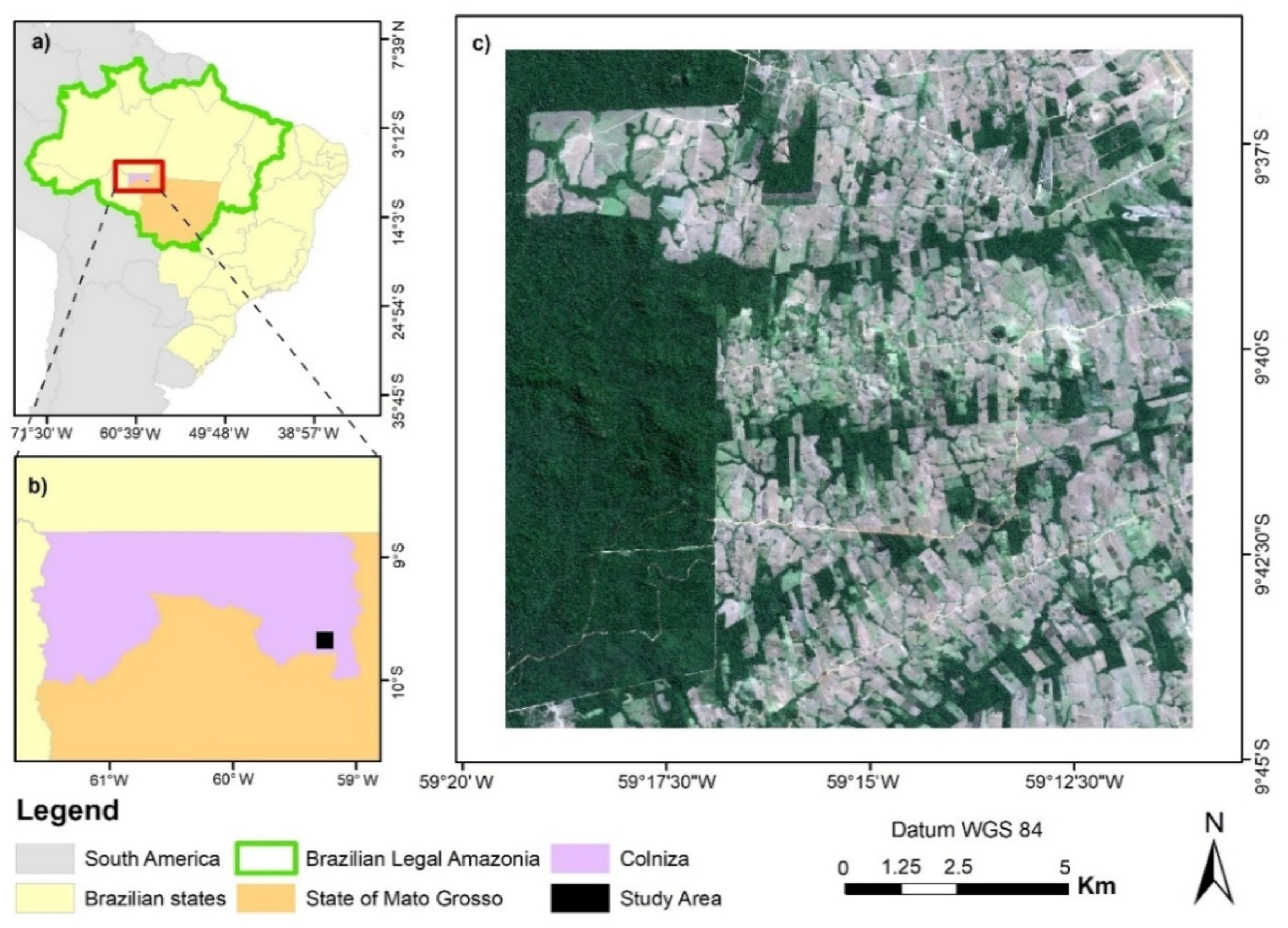
2.1. Study Area

The study area comprises a region of approximately 24,000 ha in the eastern portion of the municipality of Colniza (Figure 1), in the northwestern part of the Mato Grosso State, between 9° 36′ 23.7″ and 9° 45′ 26.5″ south latitude and between 59° 10′ 52″ and 59° 19′ 57″ west longitude. The vegetation consists of dense ombrophilous forests [40]. The climate, according to the Köppen’s climate classification system, is Am, that is, tropical (hot and humid) with a short dry season. The rainy season corresponds to the months of October to May, with the mean annual rainfall varying from 2100 to 2500 mm [41].

The municipality of Colniza presents approximately 80% of its territory still covered by primary forest [42]. About 25% of its land is covered by three indigenous lands. However, together with the neighboring municipality of Aripuanã, it is the current deforestation hotspot of the Brazilian Amazon, especially along the BR-174 highway, in the eastern part of the municipality, and where our study area is located nearby. Colniza is already facing intense landscape fragmentation [43].

2.2. Satellite Images

We selected Single Look Complex (SLC) Level 1.1, L-band ALOS/PALSAR-2 satellite images acquired on 24 March 2018 at the StripMap mode, with a spatial resolution of 6.25 m, HH and HV polarizations (hereafter refered to L-HH and L-HV polarizations, respectively), and an incidence angle of 36.6°. Another SLC SAR image selected for this study was the one acquired by the C-band Sentinel-1A satellite on 2 March 2018, with the Interferometric Wide (IW) acquisition mode, a spatial resolution of 14.05 m, VV and VH polarizations (hereafter referred to as C-VV and C-VH polarizations, respectively), and an incidence angle of 40.8°.

Two dry-season optical images, acquired by the Sentinel-2 Multispectral Instrument Image (MSI) and the China-Brazil Earth Resources Satellite (CBERS-4) data were also selected. The Sentinel-2 image was acquired on 27 July 2018, with the spatial resolution of 10 m. In this study, we selected the spectral bands 2, 3, and 4 (blue, green, and red bands, respectively). The CBERS-4 data were acquired by the wide-scan multispectral and panchromatic camera (WPM) on 9 July 2018, with the spatial resolutions of 10 m and 5 m, respectively. Drusch et al. [44] and INPE [45] provide technical details of Sentinel-2 and CBERS-4 satellites, respectively.

2.3. Methods

Figure 2 shows the main steps of the methodological approach considered in this study. The ground truth data were obtained from the data provided by the TerraClass and PRODES projects with the support of visual interpretation of the CBERS-4 image. The SAR images acquired by the ALOS-2 and Sentinel-1 satellites were pre-processed using the ESA’s Sentinel Application Platform (SNAP) 7.0 software and classified by the Random Forest (RF) and Support Vector Machine (SVM) classifiers, after we performed texture attribute selection based on the Principal Component Analysis (PCA). The accuracies of the classifications were analyzed through the confusion matrix.

2.3.1. Pre-Processing

The radiometric calibration of each L-HH- and L-HV-polarized image was carried out to obtain the backscattering coefficients (σ⁰) in the ground range (Equation (1)):

$${\sigma }^0=10 lo{g}_{10}\mathrm{(}{I}^2+Q^2\mathrm{)}+C{F}_1-A$$

(1)

where 𝐼 and 𝑄 are the real and imaginary parts of the complex images; 𝐶𝐹 is the radiometric calibration factor (−83 dB); 𝐴 is the conversion factor (32 dB) [46].

The ALOS-2 images were also filtered with the GammaMap filter to reduce speckle [47,48] using a 5 × 5 window size. The geometric correction was performed through geocoding, using the digital elevation model (DEM) produced by the Shuttle Radar Topography Mission (SRTM) and made available at the 90 m spatial resolution.

The C-VV- and C-VH-polarized images were pre-processed through the Terrain Observation with Progressive Scans (TOPSAR) split and orbit correction algorithm and selecting a smaller subarea to minimize the computational effort. Then, the procedures of deburst and radiometric calibration were applied in this software. Subsequent speckle filtering by the GammaMap filter was applied also using a 5 × 5 window size. The last procedure consisted of geometric correction through geocoding, using the same process performed for the ALOS-2 image.

2.3.2. Feature Selection

The identification of SV in the study area was based on the Gray Level Co-occurrence Matrix (GLCM), which provides textural information based on second-order statistics. The GLCM is a matrix of relative frequency P(i,j,d,θ) that considers two neighboring pixels separated by the distance d and with orientation θ from each other in a sub-region of the image, one being gray scale pixel i and the other the gray scale pixel j. Four adjacencies are defined: horizontal (0°), vertical (90°), and two diagonals (45° and 135°) [49,50]. From each matrix, it is possible to extract the following textural features, which are widely used in the literature [51]:

$$\mathrm{Entropy} \mathrm{(}\mathrm{Entr}\mathrm{)}={{\displaystyle \sum }}_{i,j}{p}_{\mathrm{(}i,j\mathrm{)}}log\left\{p_{\mathrm{(}i,j\mathrm{)}}\right\}$$

(2)

$$\mathrm{Homogeneity} \mathrm{(}\mathrm{Homo}\mathrm{)}={{\displaystyle \sum }}_{i,j}\frac{1}{1+{\mathrm{(}i-j\mathrm{)}}^2}{p}_{\mathrm{(}i,j\mathrm{)}}$$

(3)

$$\mathrm{Variance} \mathrm{(}\mathrm{Vari}\mathrm{)}={{\displaystyle \sum }}_{i,j}{\mathrm{(}i-\mu \mathrm{)}}^2{p}_{\mathrm{(}i,j\mathrm{)}}$$

(4)

$$\mathrm{Correlation} \mathrm{(}\mathrm{Corr}\mathrm{)}={{\displaystyle \sum }}_{n=0}^{Ng-1}{n}^2\left\{\begin{array}{c}{{\displaystyle \sum }}_i^{Ng}{{\displaystyle \sum }}_j^{Ng}{p}_{\mathrm{(}ij\mathrm{)}}\\ \left|i-j\right|=n\end{array}\right\}$$

(5)

$$\mathrm{Mean}={{\displaystyle \sum }}_{i,j}i\mathrm{(}{p}_{\mathrm{(}i,j\mathrm{)}}\mathrm{)}$$

(6)

$$\mathrm{Energy} \mathrm{(}\mathrm{Ener}\mathrm{)}={{\displaystyle \sum }}_{i,j}{p}_{(i,j^2)}$$

(7)

$$\mathrm{Contrast} \mathrm{(}\mathrm{Cont}\mathrm{)}={{\displaystyle \sum }}_{i,j}{p}_{\mathrm{(}i,j\mathrm{)}}{\mathrm{(}i-j\mathrm{)}}^2$$

(8)

$$\mathrm{Angular} \mathrm{Sec}\mathrm{ond} \mathrm{Moment} \mathrm{(}\mathrm{ASMO}\mathrm{)}={{\displaystyle \sum }}_{i,j}\left\{p_{{\mathrm{(}i,j\mathrm{)}}^2}\right\}$$

(9)

$$\mathrm{Dissimilarity} \mathrm{(}\mathrm{Diss}\mathrm{)}={{\displaystyle \sum }}_{i,j}{p}_{\mathrm{(}i,j\mathrm{)}}\left|i-j\right|$$

(10)

where $p_{ij}$ is the input value in the normalized GLCM; $N_g$ represents the different gray levels of the image.

These textural analyses were applied to the both ALOS/PALSAR-2 and Sentinel-1 data. According to the previous studies [52,53,54], the selected window size in the GLCM textural analysis can impact the results of LULC classifications. Small windows can amplify the amount of noise in the texture image, while larger windows can smooth the texture variation, degrading the quality of texture attributes [53,55]. Thus, four different window sizes were tested for each set of texture attributes at the 64-bit quantization level (5 × 5, 7 × 7, 9 × 9, and 11 × 11).

2.3.3. Principal Component Analysis

PCA is a technique that reduces data dimensionality by concentrating as much variance as possible in the first components based on a linear transformation [56]. In this study, in order to reduce the number of variables to be considered in the machine learning classification, we applied the PCA technique for the GLCM texture attributes. Then, we selected the first principal component (PC1) and the second principal component (PC2) to run the RF and SVM algorithms, which corresponds to same methodology applied by Wiederkehr et al. [57]. A total of 10 experiments were carried out with the SAR images (

Table 1. Parameters of the classification experiments with SAR data.

Sensor	Experiment	Data Composition	GLCM Window Size
ALOS/PALSAR-2	A1	HH + HV	-
	A2	HH + HV + GLCMPC1 + GLCMPC2	5 × 5
	A3	HH + HV + GLCMPC1 + GLCMPC2	7 × 7
	A4	HH + HV + GLCMPC1 + GLCMPC2	9 × 9
	A5	HH + HV + GLCMPC1 + GLCMPC2	11 × 11
Sentinel-1	S1	VV + VH	-
	S2	VV + VH + GLCMPC1 + GLCMPC2	5 × 5
	S3	VV + VH + GLCMPC1 + GLCMPC2	7 × 7
	S4	VV + VH + GLCMPC1 + GLCMPC2	9 × 9
	S5	VV + VH + GLCMPC1 + GLCMPC2	11 × 11

).

The texture attributes have different ranges of values among themselves. To avoid overvaluing the attributes presenting higher values, we normalized all attributes in the [0−1] interval, according to the approach described by Soares et al. [58] and Azevedo et al. [55].

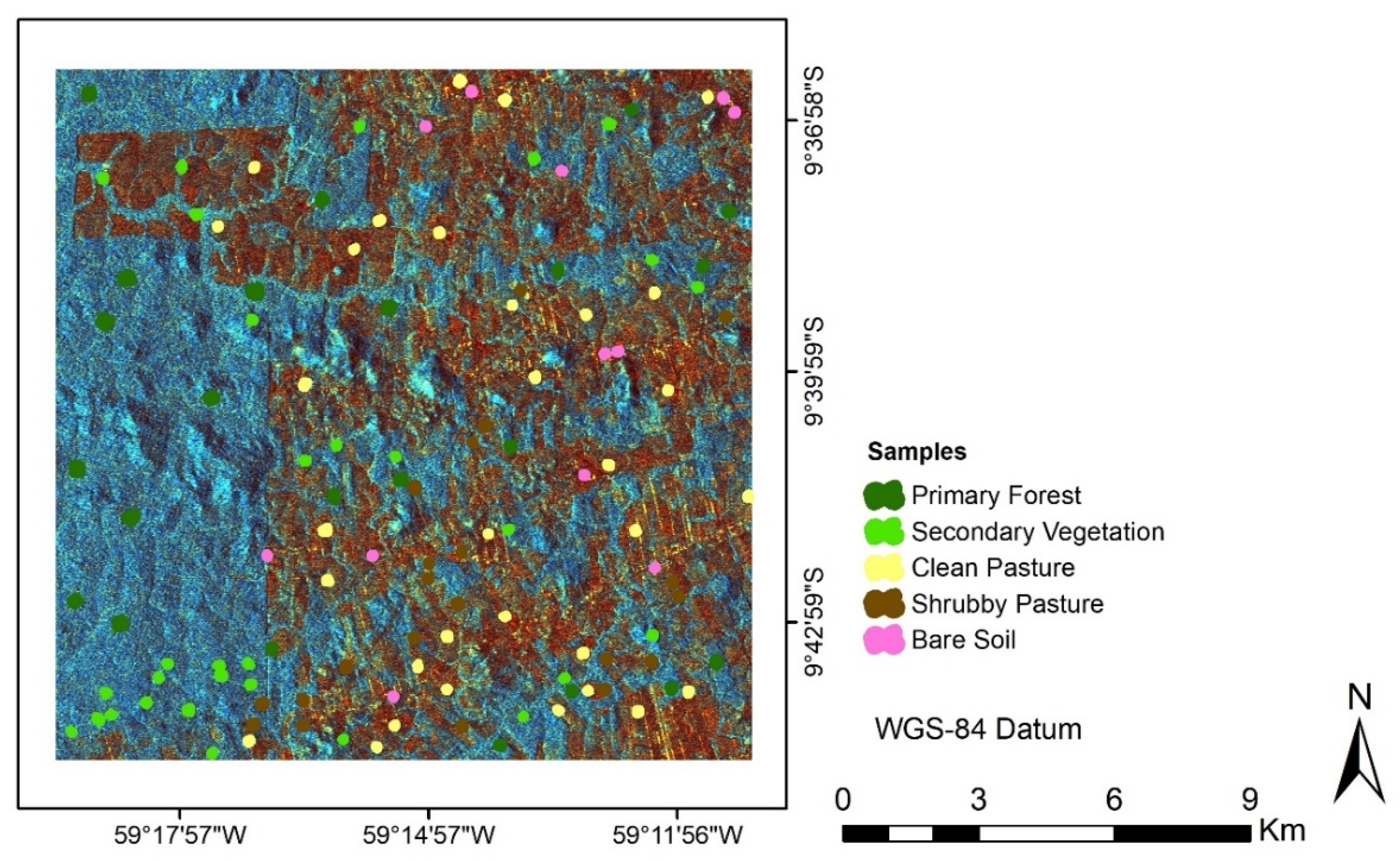
2.3.4. Reference Data and Sample Selection

Initially, a set of 122 irregular polygons were manually delimited based on the LULC classes mapped by the TerraClass project (year: 2014) and the deforestation data produced by the PRODES project (period: 2015−2018), in order to perform the image classification. The TerraClass project is composed of 17 classes; however, only the following classes that are found in the study area were considered:

• Primary Forest (PF): areas of upland, broadleaf rainfall forests and gallery forests along drainages with no evidence of human activities;
• Secondary Vegetation (SV): clear-cut forests that are regrowing as consequence of abandonment (see more details in the Introduction section);
• Clean Pasture (CP): well-managed pastures for beef production;
• Shrubby Pasture (SP): poorly managed pastures for beef production, with the presence of weeds; and
• Bare Soil (BS): relatively small areas without vegetation cover, mostly along the roads.

The number of samples for each LULC classes was defined taking into consideration the proportion of size of each class, following the recommendations of Stehman [59] and Olofsson et al. [60], who indicated four different approaches for sample allocation: proportional, equal, optimal and power allocation. Thus, a set of 122 polygons was manually drawn in the ArcGIS™ software by overlaying the TerraClass and PRODES maps in the RGB color composite of bands 6, 7, and 8 of the CBERS-4A satellite fused with the 5 m panchromatic band by the Gram–Schmidt technique available in the ENVI 5.0™ image processing software. In terms of the number of Sentinel-1 pixels, 2844 pixels were selected in the PF class; 1782 pixels in the SV; 2296 pixels in the CP; 834 pixels in the SP; 168 pixels in the BS (Figure 3). In terms of ALOS/PALSAR-2 pixels, 5771 pixels were selected in the PF class; 3454 pixels in the SV; 4633 pixels in the CP; 1588 pixels in the SP; 298 pixels in the BS. These different sets of pixels correspond to the approximate proportion of LULC classes mapped in the study area by the TerraClass project: SV = 18%; CP = 31%; SP = 11%; BS = 2%. Seventy-five percent of the sampling points were used to train the image classifiers while the remaining points were used to validate the results of the classification.

Images from the panchromatic band onboard the CBERS-4 satellite were used as a reference. A true composite was performed with the multispectral bands (10 m resolution) that were later merged through the Gram–Schmidt fusion technique with the panchromatic band with a 5 m spatial resolution.

2.3.5. Machine Learning Classifications

In this study, the image classifications were performed using the RF and SVM classifiers available in the EnMAP-Box software [61]. They were less sensitive to the speckle-affected SAR data, showing good classification results involving LULC dynamics in forests [62]. The RF algorithm uses decision trees to increase classification accuracy through many combinations of random subsets of trees [63]. It constitutes an ensemble and bagging algorithm, ensemble because it gathers and employs a set of regression trees classifiers and bagging because decision trees are created from subsets of the same sample set, with replacement [64]. In this study, we carried out preliminary tests with 100, 500, and 1000 trees. Although the classification accuracy increased with the increasing number of trees, we opted to use 500 trees in all classifications because of the best compromise between computational effort and model accuracy. Previous studies also have recommended 500 trees [64,65].

We evaluated the accuracy of the RF classification using an approach in which the RF algorithm collects approximately 75% of data as a training set while the remaining is left out, a procedure known as out-of-bag (OOB). The OOB samples are then directed to trees that have not been used by the classifier yet. The difference between the expected and the real class is used to estimate the classification error [63]. This method is considered unbiased because, as the number of trees increases, the error tends to decrease to a certain threshold. The importance of each variable in the classification process, in raw and normalized values, is calculated from the OOB samples. We considered the number of variables as the default value, which corresponded to the square root of the total number of input variables [64].

The SVM algorithm is a nonlinear classifier that is trained to find an optimal classification hyperplane. It minimizes the upper bound of the classification error and maximizes the distance of the data points of each class to the ideal separation linear hyperplane of the axes created from each variable [66]. The SVM model is optimized to look for a non-linear hyperplane in a multidimensional feature space using a kernel function [67]. The most used kernel functions are the linear, polynomial, radial basis function (RBF), and sigmoid functions [68]. In this study, we selected the RBF function, which has two predefined parameters, the cost (C) and the gamma (γ). Both parameters depend on the data range and distribution and differ from one classification to the other. In order to find the optimum C and γ parameters, a two-dimensional grid search with internal validation was performed within the EnMAP-Box software, for each classification [69].

2.3.6. Accuracy Analysis

The classification results from the experiments were analyzed through the confusion matrices (user’s and producer’s accuracies), Kappa coefficient, and overall accuracy (OA), with a level of significance of 5%. For the best classification result with the RF algorithm, the ranking of predicted variables showing the most important features was calculated.

3. Results

3.1. C- and L-Band Backscatter Coefficients

Figure 4 shows the average values and corresponding standard deviations of the backscattering coefficients of C-VV, C-VH, L-HH, and L-HV data sets obtained from the calibration sites. Co-polarized signals (L-HH and C-VV) were higher than those from the cross-polarized signals (L-HV and C-VH). This was somewhat expected since the backscattering process, involving cross-polarized energy, is mainly related to the volumetric scattering from the canopy, attenuating the SAR signal returned to the antenna [70]. In the case of co-polarized energy, most of the backscattering process is related to the stronger signal returns from trunks, branches, and leaves located in the upper part of the canopy.

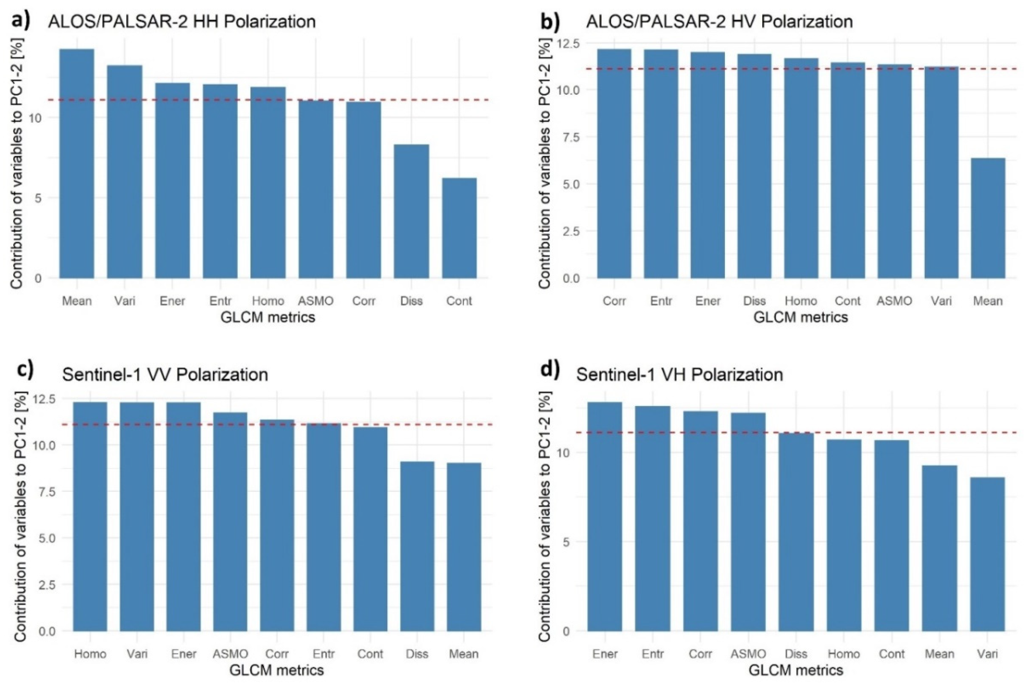
3.2. Most Relevant Texture Attributes of SAR Images

Figure 5 presents the ranking of the percentage of contribution of most important texture attributes of each SAR images considered in this study. The total contribution of first two principal components varied from 74.2% (L-HH polarization) to 98.4% (C-VV polarization). For the L-HH polarization, the variations explained by the first two principal components were 48.9% and 25.3%, respectively. For the L-HV polarization, the variations in PC1 and PC2 were 71.4% and 17.6%, respectively. For the C-VV polarization, the variations explained by PC1 and PC2 were 87.6% and 10.8%, respectively while for the C-VH polarization, the variations in PC1 and PC2 were 63.7% and 20.5%, respectively. The order of the importance of textural attributes varied according to the polarization. These texture features are considered the most important among all texture attributes analyzed for the SV samples and were grouped according to the results of each polarization.

Table 2. Organization of texture features used in each experiment, after PCA analysis.

Satellite	Experiments	Data Composition	No. Images
ALOS/ PALSAR-2	A1	L-HH + L-HV	2
	A2, A3, A4, and A5	L-HH + L-HH(mean) + L-HH(vari) + L-HH(ener) + L-HH(entr) + L-HH(homo) + L-HV + L-HV(corr) +L-HV(entr) + L-HV(ener) + L-HV(diss) + L-HV(homo) + L-HV(contr) + L-HV(ASMO) + L-HV(vari)	15
Sentinel-1	S1	C-VV + C-VH	2
	S2, S3, S4, and S5	C-VV + C-VV(homo) + C-VV(vari) + C-VV(ener) + C-VV(ASMO) + C-VV(corr) + C-VH + C-VH(ener) + C-VH(entr) + C-VH(corr) + C-VH(ASMO)	11

shows how each set of texture features that was used in the experiments was organized. The ALOS/PALSAR-2 images had more texture attributes included in relation to the Sentinel-1 images, mainly regarding the HV cross-polarization.

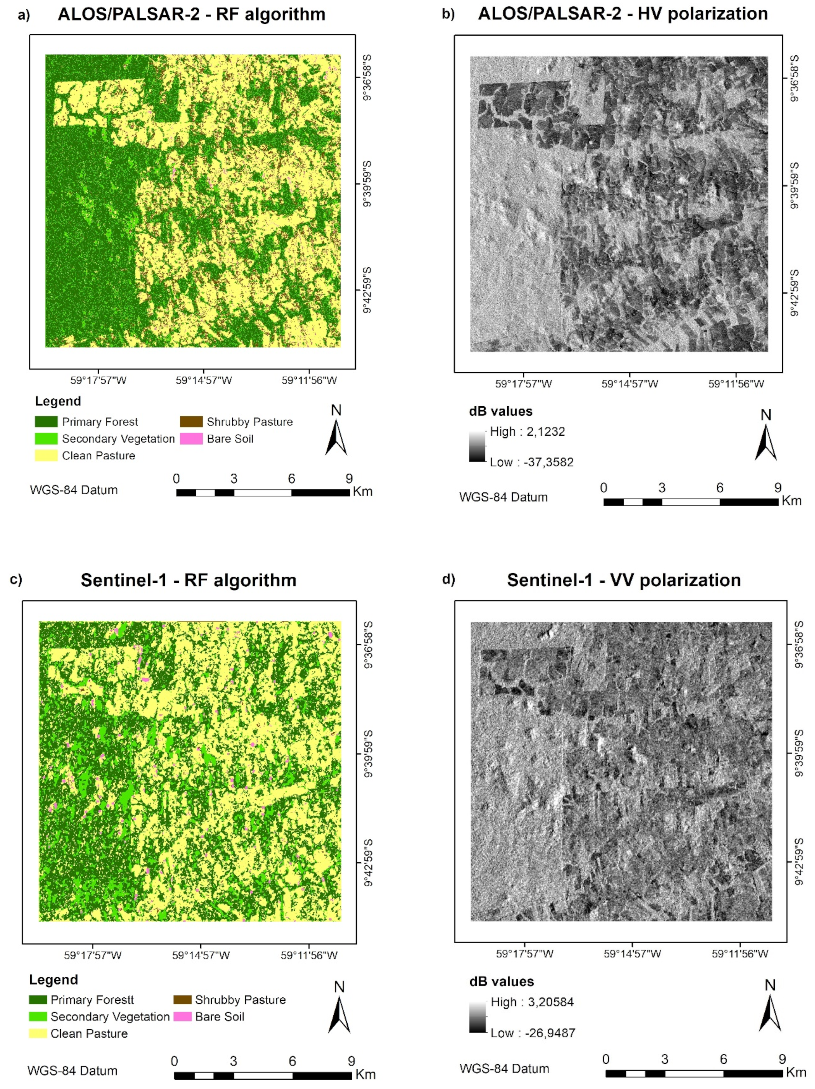
3.3. Random Forest and Support Vector Machine Classification Results for the SAR Data

Table 3. Overall accuracy (OA) and Kappa coefficient for the Random Forest classification experiments involving ALOS/PALSAR-2 and Sentinel-1 data sets. PF = primary forest; SV = secondary vegetation; CP = clean pasture; SP = shrubby pasture; BS = bare soil. See details of the experiments in Table 1.

Experiment	User’s Accuracy (%)					Producer’s Accuracy (%)					OA %	Kappa
	PF	SV	CP	SP	BS	PF	SV	CP	SP	BS
A1	67.52	59.87	75.52	52.99	40.00	81.00	44.29	86.55	32.05	8.60	67.75	0.54
A2	70.79	72.44	74.72	63.70	75.00	90.50	43.59	94.59	20.99	3.23	72.16	0.60
A3	74.58	73.43	80.74	74.68	60.00	91.58	53.53	92.53	39.95	9.68	76.29	0.66
A4	77.50	77.87	84.60	76.31	70.59	91.94	58.69	93.77	55.98	12.90	79.62	0.71
A5	82.60	84.52	86.63	82.64	91.67	95.15	68.32	95.16	67.72	11.83	84.20	0.78
S1	59.11	62.18	65.74	57.69	28.57	72.28	53.33	72.52	27.03	8.00	61.35	0.45
S2	57.45	66.22	58.36	72.41	80.00	72.28	43.56	75.95	18.92	32.00	59.74	0.42
S3	64.62	80.72	67.35	75.56	71.43	82.88	59.56	75.57	30.63	40.00	68.72	0.55
S4	66.60	78.28	79.07	73.58	91.67	85.05	68.89	77. 86	35.14	44.00	72.86	0.61
S5	75.82	81.16	88.89	84.31	90.00	92.99	76.02	85.41	42.57	47.37	81.07	0.73

shows the user’s accuracy, producer’s accuracy, OA, and Kappa coefficient for each experiment performed with the RF algorithm. In general, the performance of the ALOS/PALSAR-2 data was higher than that from Sentinel-1 data. The best result of the RF classification involving ALOS/PALSAR-2 data was achieved by the Experiment A5 (overall accuracy of 84.20%; Kappa coefficient of 0.78), while for the Sentinel-1 data, the best result was obtained by the Experiment S5 (overall accuracy of 81.07%; Kappa coefficient of 0.73). We can note an improvement when texture attributes were added to the backscatter values in both the ALOS-2 and Sentinel-1 data.

Table 4. Overall accuracy (OA) and Kappa coefficient for the Support Vector Machine classification experiments involving ALOS/PALSAR-2 and Sentinel-1 data sets. PF = primary forest; SV = secondary vegetation; CP = clean pasture; SP = shrubby pasture; BS = bare soil. See details of the experiments in Table 1.

Experiment	User’s Accuracy (%)					Producer’s Accuracy (%)					OA %	Kappa
	PF	SV	CP	SP	BS	PF	SV	CP	SP	BS
A1	47.40	65.33	53.24	0.00	0.00	74.18	21.78	69.08	2.26	0.00	50.76	0.27
A2	50.17	66.33	58.42	50.00	83.33	78.53	28.89	67.56	0.90	40.00	54.69	0.33
A3	55.41	70.59	66.42	69.57	84.62	82.07	42.67	69.47	14.41	44.00	61.25	0.44
A4	65.50	75.66	71.89	63.46	81.82	81.52	63.56	77.10	29.73	36.00	69.32	0.56
A5	70.32	72.20	86.33	65.57	100.00	83.02	66.97	85.41	39.60	57.89	75.23	0.65
S1	45.92	53.12	53.25	0.00	100.00	60.16	35.06	75.08	0.00	1.04	49.89	0.28
S2	48.82	56.80	54.79	0.00	57.14	66.45	38.82	71.52	0.00	12.50	52.31	0.32
S3	50.03	60.80	57.00	0.00	42.50	69.58	42.71	69.58	0.00	17.71	54.04	0.34
S4	52.47	57.66	60.02	0.00	38.89	72.03	46.47	70.09	0.00	14.58	55.73	0.37
S5	56.79	59.89	64.83	10.00	36.54	70.60	53.06	80.26	0.25	19.79	59.74	0.43

shows the user’s accuracy, producer’s accuracy, OA, and Kappa coefficient for each experiment performed with the SVM algorithm. Again, the performance of the ALOS/PALSAR-2 data was higher than that from Sentinel-1 data in terms of the OA and Kappa coefficient. For the SV discrimination, the ALOS/PALSAR-2 presented a better performance in terms of user’s accuracy (75.66%) and producer’s accuracy (66.97%) than that from the Sentinel-1 data (user’s accuracy and producer’s accuracy of 60.80% and 53.06%, respectively). Figure 5 shows the overall accuracy (OA) and Kappa coefficient for each experiment performed with the RF algorithm and for the SVM algorithm, respectively.

Figure 6 presents the ranking of importance of each feature in the classification process based on the RF algorithm performed, considering the A5 and S5 experiments, which showed the highest overall accuracy in the previous test. In both classifications, the GLCM correlation related to the cross-polarizations (HV and VH, respectively) contributed more to the RF classification.

Figure 7 illustrates the result of the best accuracies found with the ALOS/PALSAR-2 (Experiment A5, RF) and Sentinel-1 (Experiment S5, RF) data. We note a predominance of PF in the western part of the study area and the CP in the rest of the study area. The SV and SP occupy less than 25% of the study area (Figure 8) and are distributed throughout the study area in relatively small areas. The small extension of BS occurs in the western part of the study area.

4. Discussion

Overall, the backscattering coefficients obtained in this study are in agreement with previous values reported by other studies conducted in different sites of the Brazilian Amazon: −7.53 dB and −12.59 dB for primary forest and ALOS-2 L-HH and L-HV images, respectively [71]; −7.53 dB and −12.45 dB for secondary forest and ALOS-2 L-HH and L-HV images, respectively [72]; −14.81 dB and −22 dB for cultivated pastures and ALOS-2 L-HH and L-HV images, respectively [71]. The lower values of the backscattering coefficients for bare soils and clean pastures are related to the lack or low levels of biomass. None of the SAR configurations showed a clear possibility of discriminating the SV from other LULC classes based solely on SAR amplitude (backscattering coefficients) data. This indicates the need of additional data such as the use of textural information for classifying SV.

The experiments with the ALOS/PALSAR-2 image presented a better performance than those involving Sentinel-1 data, reaching a maximum performance (OA of 84.2%; Kappa coefficient of 0.78) when texture attributes with 11 × 11 window size were added to the radiometric information (backscattering coefficient). These findings agree with the results found by Li et al. [73] who analyzed radiometric images and their textures obtained by the L-band ALOS/PALSAR-1 and C-band RADARSAT (C-band SAR) satellites for LULC classification in Altamira, Pará, Brazil. They concluded that the L-band data provided better LULC classification than the C-band data, regardless of the classification algorithm. Mercier et al. [74] and Nicolau et al. [75] also found significant confusion in discriminating secondary vegetation and forest based on Sentinel-1 data sets acquired over the study areas located in the municipality of Paragominas, Pará State, Brazil, and Madre de Dios region, Peru, respectively.

In this study, we noted that the largest window size presented the best classification results. According to Zhou et al. [76], textural attributes derived from the GLCM method are highly sensitive to the moving window size and the best criterion to set the value of the moving window size is still not fully understood. Coburn and Roberts [77] reported that large window sizes are more suitable when landscape is heterogeneous, and vice-versa. This last statement may explain our best results for the largest window size.

The use of SAR textural attributes improved the discrimination capability of different LULC classes found in the study area. Zhu et al. [78] reported an improvement from 31% to 72% in classification accuracy when texture metrics were added to the ALOS/PALSAR data in an urban and peri-urban environment (Boston, Massachusetts, USA). In the study conducted by Pavanelli et al. [79], the addition of these metrics to the ALOS/PALSAR-2 data sets increased the classification from 30.0% to 44.6%. According to these authors, this relatively low accuracy was due to the much higher number of classes selected for classification (17) than in the other studies. Here, it is important to note that textural images do not assure improvements in all LULC classes because it varies with the landscape characteristics and image acquisition modes [73]. Another important aspect pointed out by these authors is the selection of a suitable size of the moving window. As the sizes of LULC patches vary greatly, typically less than 1 ha for bare soil to hundreds of hectares of pastures and PF in our study area, no window size will be perfect to discriminate all LULC classes at once.

In this study, the RF outperformed the SVM classifier to discriminate the five LULC classes by 14% of overall accuracy for both ALOS-2 and Sentinel-1 data sets, considering the five experiments. The performance of discriminating SV was also higher for the RF algorithm: 3.6% and 16% higher in terms of OA for ALOS-2 and Sentinel-1 data sets, respectively. Previous studies highlight the low sensitivity to feature selection, simple parameterization, and short calculation time as being the main advantages of the RF classifier method [64,74,80].

One of the most difficult aspects of this study was the gathering of reliable ground truth data for training and validation of two selected non-parametric, machine learning algorithms. The field campaign was very complicated to be conducted due to the poor road accessibility during the rainy season. Besides, there was no forest inventory available in the study area. We tried to use the best ancillary data, available from the TerraClass project, however, there was a four-year delay between the last LULC map produced by this project (2014) and the satellite overpasses (2018). This may contribute to reducing the accuracy of our final classifications.

5. Conclusions

This study evaluated the potential of C- and L-band SAR data acquired in the rainy season to discriminate SV in a region considered to be the new hotspot of clear-cut deforestation in the Brazilian Amazon. The approach used in this research brings some important contributions to the development of a SAR-based system to monitor the near-real time re-suppression of SV in the Brazilian Amazon. First, we demonstrated the better potential of L-band ALOS/PALSAR-2 data in comparison with the C-band Sentinel-1 data for discriminating different LULC representative classes of the Brazilian Amazon. Second, the ability of the RF classifier to discriminate SV was higher when compared to the SVM classifier. Third, the use of both amplitude and texture attributes is highly recommended to improve the accuracy of the classification. Further research is needed to test the performances of other classification methods such as the U-NET that is based on semantic segmentation, the deep learning-based Convolutional Support Vector Machine (CSVM) or the Convolutional Neural Network-Multilayer Perceptron (CNN-MLP) data augmentation technique. Future research is also demanded to test the different polarimetric decompositions and interferometric techniques to discriminate between areas of secondary vegetation.

References

1. INPE. TerraBrasilis. PRODES (Deforestation). 2022. Available online: http://terrabrasilis.dpi.inpe.br/app/dashboard/deforestation/biomes/legal_amazon/rates (accessed on 24 June 2022).
2. Sauer, S. Soy expansion into the agricultural frontiers of the Brazilian Amazon: The agribusiness economy and its social and environmental conflits. Land Use Policy 2018, 79, 326–338. [Google Scholar] [CrossRef]
3. Miranda, J.; Börner, J.; Kalkuhl, M.; Soares-Filho, B. Land speculation and conservation policy leakage in Brazil. Environ. Res. Lett. 2019, 14, 045006. [Google Scholar] [CrossRef]
4. Arias, M.E.; Farinosi, F.; Lee, E.; Livino, A.; Briscoe, J.; Moorcroft, P.R. Impacts of climate change and deforestation on hydropower planning in the Brazilian Amazon. Nat. Sustain. 2020, 3, 430–436. [Google Scholar] [CrossRef]
5. Skidmore, M.E.; Moffette, F.; Rausch, L.; Christie, M.; Munger, J.; Gibbs, H.K. Cattle ranchers and deforestation in the Brazilian Amazon: Production, location, and policies. Global Environ. Chang. 2021, 68, 102280. [Google Scholar] [CrossRef]
6. Pereira, E.J.A.L.; Ferreira, P.J.S.; Ribeiro, L.C.S.; Carvalho, T.S.; Pereira, H.B.B. Policy in Brazil (2016–2019) threaten conservation of the Amazon rainforest. Environ. Sci. Policy 2019, 100, 8–12. [Google Scholar] [CrossRef]
7. Trancoso, R. Changing Amazon deforestation patterns: Urgent need to restore command and control policies and market interventions. Environ. Res. Lett. 2021, 16, 041004. [Google Scholar] [CrossRef]
8. Corlett, R.T. What is secondary forest? J. Trop. Ecol. 1994, 10, 445–447. [Google Scholar] [CrossRef]
9. CDB. Definitions: Indicative Definitions Taken from the Report of the Ad Hoc Technical Expert Group on Forest Biological Diversity. 2006. Available online: https://www.cbd.int/forest/definitions.shtml (accessed on 24 June 2022).
10. FAO. Global Forest Resources Assessment 2020; Main Report; FAO: Rome, Italy, 2020; 186p. [Google Scholar]
11. Almeida, C.A.; Coutinho, A.C.; Esquerdo, J.C.D.M.; Adami, M.; Venturieri, A.; Diniz, C.G.; Dessay, N.; Durieux, L.; Gomes, A.R. High spatial resolution land use and land cover mapping of the Brazilian Legal Amazon in 2008 using Landsat-5/TM and MODIS data. Acta Amazon. 2016, 46, 291–302. [Google Scholar] [CrossRef]
12. INPE. TerraClass. Projetos e Pesquisas. 2019a. Available online: http://www.inpe.br/cra/projetos_pesquisas/dados_terraclass.php (accessed on 24 June 2022).
13. Chazdon, R.L.; Broadbent, E.N.; Rozendaal, D.M.; Bongers, F.; Zambrano, A.M.A.; Aide, T.M.; Balvanera, P.; Becknell, J.M.; Boukili, V.; Bracalion, P.H.S.; et al. Carbon sequestration potential of second-growth forest regeneration in the Latin American tropics. Sci. Adv. 2016, 2, e1501639. [Google Scholar] [CrossRef]
14. Bongers, F.; Chazdon, R.; Poorter, L.; Peña-Claros, M. The potential of secondary forests. Science 2015, 348, 642–643. [Google Scholar] [CrossRef]
15. Strassburg, B.B.N.; Latawiec, A.E.; Barioni, L.G.; Nobre, C.A.; Silva, V.P.; Valentim, J.F.; Vianna, M.; Assa, E.D. When enough should be enough: Improving the use of current agricultural lands could meet production demands and spare natural habitats in Brazil. Glob. Environ. Change 2014, 28, 84–97. [Google Scholar] [CrossRef]
16. Klemick, H. Shifting cultivation, forest fallow, and externalities in ecosystem services: Evidence from the Eastern Amazon. J. Environ. Econ. Manag. 2011, 61, 95–106. [Google Scholar] [CrossRef]
17. Nunes, S.; Oliveira, L., Jr.; Siqueira, J.; Morton, D.C.; Souza, C.M., Jr. Unmasking secondary vegetation dynamics in the Brazilian Amazon. Environ. Res. Lett. 2020, 15, 034057. [Google Scholar] [CrossRef]
18. Soares-Filho, B.; Rajão, R.; Macedo, M.; Carneiro, A.; Costa, W.; Coe, M.; Rodrigues, H.; Alencar, A. Cracking Brazil’s forest code. Science 2014, 344, 363–364. [Google Scholar] [CrossRef]
19. Diniz, C.G.; Souza, A.A.A.; Santos, D.C.; Dias, M.C.; Luz, N.C.; Moraes, R.V.; Maia, J.S.; Gomes, A.R.; Narvaes, I.S.; Valeriano, D.M.; et al. DETER-B: The new Amazon near real-time deforestation detection system. IEEE J. Sel. Top. Appl. Earth Obs. Remote Sens. 2015, 8, 3619–3628. [Google Scholar] [CrossRef]
20. IMAZON. Sistema De Alerta De Desmatamento (Sad)—Maio De 2022. Available online: https://imazon.org.br/publicacoes/sistema-de-alerta-de-desmatamento-sad-maio-de-2022/ (accessed on 24 June 2022).
21. Souza, C.M., Jr.; Shimbo, J.Z.; Rosa, M.R.; Parente, L.L.; Alencar, A.A.; Ruddorff, B.F.T.; Hasenack, H.; Matsumoto, M.; Ferreira, L.G.; Souza-Filho, P.W.M.; et al. Reconstructing three decades of land use and land cover changes in Brazilian biomes with Landsat archive and Earth Engine. Remote Sens. 2020, 12, 2735. [Google Scholar] [CrossRef]
22. Lucas, R.M.; Xiao, X.; Hagen, S.; Frolking, S. Evaluating TERRA-1 MODIS data for discrimination of tropical secondary forest regeneration stages in the Brazilian Legal Amazon. Geophys. Res. Lett. 2002, 29, 1–4. [Google Scholar] [CrossRef]
23. Asner, G.P.; Rudel, T.K.; Aide, T.M.; Defries, R.; Emerson, R. A Contemporary assessment of change in humid tropical forests. Conserv. Biol. 2009, 23, 1386–1395. [Google Scholar] [CrossRef]
24. Wang, J.; Yang, D.; Detto, M.; Nelson, B.W.; Chen, M.; Guan, K.; Wu, S.; Yan, Z.; Wu, J. Multi-scale integration of satellite remote sensing improves characterization of dry-season green-up in an Amazon tropical evergreen forest. Remote Sens. Environ. 2020, 246, 111865. [Google Scholar] [CrossRef]
25. Vieira, I.C.G.; Gardner, T.; Ferreira, J.; Lees, A.C.; Barlow, J. Challenges of governing second-growth forests: A case study from the Brazilian Amazonian State of Pará. Forests 2014, 5, 1737–1752. [Google Scholar] [CrossRef] [Green Version]
26. Shimada, M.; Isoguchi, O.; Tadono, T.; Isono, K. PALSAR radiometric and geometric calibration. IEEE Trans. Geosci. Remote Sens. 2009, 47, 3915–3932. [Google Scholar] [CrossRef]
27. Watanabe, M.; Koyama, C.; Hayashi, M.; Nagatani, I.; Shimada, M. Early-stage deforestation detection in the tropics with L-band SAR. IEEE J. Sel. Top. Appl. Earth Obs. Remote Sens. 2018, 11, 1–7. [Google Scholar] [CrossRef]
28. Watanabe, M.; Koyama, C.; Hayashi, M.; Nagatani, I.; Tadono, T.; Shimada, M. Refined algorithm for forest early warning system with ALOS-2/PALSAR-2 ScanSAR data in tropical forest regions. Remote Sens. Environ. 2021, 265, 112643. [Google Scholar] [CrossRef]
29. Cassol, H.L.G.; Aragão, L.E.O.C.; Moraes, E.C.; Carriras, J.M.B.; Shimabukuro, Y.E. Quad-pol advanced land observing satellite/phased array L-band synthetic aperture radar-2 (ALOS/PALSAR-2) data for modeling secondary forest above-ground biomass in the central Brazilian Amazon. Int. J. Remote Sens. 2021, 42, 4985–5009. [Google Scholar] [CrossRef]
30. Leckie, D.G.; Ranson, K.J. Forestry applications using imaging SAR. In Principles and Application of Imaging Radar. Manual of Remote Sensing, 3rd ed.; Henderson, F.M., Lewis, A.J., Eds.; John Wiley & Sons: Hoboken, NJ, USA, 1998. [Google Scholar]
31. Torres, R.; Snoeij, P.; Geudtner, D.; Bibby, D.; Davidson, M.; Attema, E.; Potin, P.; Rommen, B.; Floury, N.; Brown, M.; et al. GMES Sentinel-1 mission. Remote Sens. Environ. 2012, 120, 9–24. [Google Scholar] [CrossRef]
32. Doblas, J.; Shimabukuro, Y.; Sant´Anna, S.; Carneiro, A.; Aragão, L.; Almeida, C. Optimizing near real-time detection of deforestation on tropical rainforests using Sentinel-1 data. Remote Sens. 2020, 12, 3922. [Google Scholar] [CrossRef]
33. Hoekmann, D.; Kooij, B.; Quiñones, M.; Vellekoop, S.; Carolita, I.; Budhiman, S.; Arief, R.; Roswintiarti, O. Wide-area near-real-time monitoring of tropical forest degradation and deforestation using Sentinel-1. Remote Sens. 2020, 12, 3263. [Google Scholar] [CrossRef]
34. Silva, C.A.; Guerrisi, G.; Del Frate, F.; Sano, E.E. Near-real time deforestation detection in the Brazilian Amazon with Sentinel-1 and neural networks. Eur. J. Remote Sens. 2022, 55, 129–149. [Google Scholar] [CrossRef]
35. Kuplich, T.M. Classifying regenerating forest stages in Amazônia using remotely sensed images and a neural network. For. Ecol. Manage. 2006, 234, 1–9. [Google Scholar] [CrossRef]
36. Carreiras, J.M.B.; Jones, J.; Lucas, R.M.; Shimabukuro, Y.E. Mapping major land cover types and retrieving the age of secondary forests in the Brazilian Amazon by combining single-date optical and radar remote sensing data. Rem. Sens. Environ. 2017, 194, 16–32. [Google Scholar] [CrossRef] [Green Version]
37. Doblas, J.; Reis, M.S.; Belluzzo, A.P.; Quadros, C.B.; Moraes, D.R.V.; Almeida, C.A.; Maurano, L.E.P.; Carvalho, A.F.A.; Sant´Anna, S.J.S.; Shimabukuro, Y.E. DETER-R: An operational near-real time tropical forest disturbance warning system based on Sentinel-1 time series analysis. Remote Sens. 2022, 14, 3658. [Google Scholar] [CrossRef]
38. Assunção, J.J.; Gandour, C. What Does the Surge in Amazon Regeneration Mean for Brazil? Climate Policy Initiative: Rio de Janeiro, Brazil, 2017; Available online: https://climatepolicyinitiative.org/publication/surge-amazon-regeneration-mean-brazil/ (accessed on 22 August 2018).
39. Aoki, Y.; Furuya, M.; Zan, F.; Doin, M.P.; Eineder, M.; Ohki, M.; Wright, T.J. L-band synthetic aperture radar: Current and future applications to Earth sciences. Earth Planets Space 2021, 73, 56. [Google Scholar] [CrossRef]
40. IBGE. Manual Técnico da Vegetação Brasileira. Manuais Técnicos em Geociências, n. 1; IBGE: Rio de Janeiro, Brazil, 2012; 274p. [Google Scholar]
41. Santos, M.V. Zoneamento sócio-econômico-ecológico: Diagnóstico sócio-econômico-ecológico do Estado de Mato Grosso e assistência técnica na formulação da 2ª aproximação; SEPLAN-MT: Cuiabá, MT, Brazil, 2000. [Google Scholar]
42. MapBiomas. MapBiomas v. 6.0. Available online: https://mapbiomas.org/en/statistics (accessed on 25 June 2022).
43. Halbgewachs, M.; Wegmann, M.; Ponte, E. A spectral mixture analysis and landscape metrics based framework for monitoring spatiotemporal forest cover changes: A case study in Mato Grosso, Brazil. Remote Sens. 2022, 14, 1907. [Google Scholar] [CrossRef]
44. Drusch, M.; Bello, U.D.; Carlier, S.; Colin, O.; Fernandez, V.; Gascon, F.; Hoersch, B.; Isola, C.; Laberinti, P.; Martimort, P.; et al. Sentinel-2: ESA´s optical high-resolution mission for GMES operational services. Remote Sens. Environ. 2012, 120, 25–36. [Google Scholar] [CrossRef]
45. INPE. CBERS 04A. 2019. Available online: http://www.cbers.inpe.br/sobre/cbers04a.php?_ga=2.99883486.151721476.1656282945-118845307.1656282944 (accessed on 26 June 2022).
46. JAXA. Calibration Results of ALOS-2/PALSAR-2 JAXA Standard Products. Available online: https://www.eorc.jaxa.jp/ALOS-2/en/calval/calval_index.htm (accessed on 8 February 2022).
47. Small, D. Flattening Gamma: Radiometric terrain correction for SAR imagery. IEEE Trans. Geosci. Remote Sens. 2011, 49, 3081–3093. [Google Scholar] [CrossRef]
48. Hagensieker, R.; Waske, B. Evaluation of multi-frequency SAR images for tropical land cover mapping. Remote Sens. 2018, 10, 257. [Google Scholar] [CrossRef]
49. Haralick, R.M.; Shanmugam, K.; Dinstein, I.H. Textural features for image classification. IEEE Trans. Syst. Man Cybern. Syst. 1973, 3, 610–621. [Google Scholar] [CrossRef]
50. Kurvonen, L.; Hallikainen, M.T. Textural information of multitemporal ERS-1 and JERS-1 SAR images with applications to land and forest type classification in boreal zone. IEEE Tran. Geosci. Remote Sens. 1999, 37, 680–689. [Google Scholar] [CrossRef]
51. Baraldi, A.; Parmiggiani, F. A refined gamma MAP SAR speckle filter with improved geometrical adaptivity. IEEE Trans. Geosci. Remote Sens. 1995, 33, 1245–1257. [Google Scholar] [CrossRef]
52. Lu, D.; Batistella, M. Exploring TM image texture and its relationships with biomass estimation in Rondônia, Brazilian Amazon. Acta Amaz. 2005, 35, 249–257. [Google Scholar] [CrossRef]
53. Sothe, C.; Almeida, C.M.; Liesenberg, V.; Schimalski, M.B. Evaluating Sentinel-2 and Landsat-8 data to map successional forest stages in a subtropical forest in southern Brazil. Remote Sens. 2017, 9, 838. [Google Scholar] [CrossRef]
54. Zakeri, H.; Yamazaki, F.; Liu, W. Texture analysis and land cover classification of Tehran using polarimetric synthetic aperture radar imagery. Appl. Sci. 2017, 7, 452. [Google Scholar] [CrossRef]
55. Azevedo, A.R.D.; Santos, J.R.D.; Gama, F.F.; Graça, P.M.L.D.A.; Mura, J.C. Caracterização de uso e cobertura da terra na Amazônia utilizando imagens duais multitemporais do COSMO-SkyMed. Acta Amaz. 2014, 44, 87–97. [Google Scholar] [CrossRef]
56. Jolliffe, I.T. Principal Component Analysis; Springer: New York, NY, USA, 2002. [Google Scholar]
57. Wiederkehr, N.C.; Gama, F.F.; Castro, P.B.; Bispo, P.D.C.; Balzter, H.; Sano, E.E.; Mura, J.C. Discriminating Forest successional stages, forest degradation, and land use in central amazon using ALOS/PALSAR-2 full-polarimetric data. Remote Sens. 2020, 12, 3512. [Google Scholar] [CrossRef]
58. Soares, J.V.; Rennó, C.D.; Formaggio, A.R.; Yanasse, C.C.F.; Frery, A.C. An investigation of the selection of texture features for crop discrimination using SAR imagery. Remote Sens. Environ. 1997, 59, 234–247. [Google Scholar] [CrossRef]
59. Stehman, S.V. Impact of sample size allocation when using stratified random sampling to estimate accuracy and area of land-cover change. Remote Sens. Lett. 2012, 3, 111–120. [Google Scholar] [CrossRef]
60. Olofsson, P.; Foody, G.M.; Herold, M.; Stehman, S.V.; Woodcock, C.E.; Wulder, M.A. Good practices for estimating area and assessing accuracy of land change. Remote Sens. Environ. 2014, 148, 42–57. [Google Scholar] [CrossRef]
61. Van der Linden, S.; Rabe, A.; Held, M.; Jakimow, B.; Leitão, P.J.; Okujeni, A.; Schwieder, S.S.; Hostert, P. The EnMAP-Box—A toolbox and application programming interface for EnMAP data processing. Remote Sens. 2015, 7, 11249–11266. [Google Scholar] [CrossRef]
62. Diniz, J.M.F.S.; Gama, F.F.; Adami, M. Evaluation of polarimetry and interferometry of Sentinel-1A SAR data for land use and land cover of the Brazilian Amazon region. Geocarto Int. 2022, 37, 1482–1500. [Google Scholar] [CrossRef]
63. Breiman, L. Random Forests. Mach. Learn. 2001, 45, 5–32. [Google Scholar] [CrossRef] [Green Version]
64. Belgiu, M.; Drăguţ, L. Random forest in remote sensing: A review of applications and future directions. ISPRS J. Photogramm. Remote Sens. 2016, 114, 24–31. [Google Scholar] [CrossRef]
65. Sheykhmousa, M.; Mahdianpari, M.; Ghanbari, H.; Mohammadimanesh, F.; Ghamisi, P.; Homayouni, S. Support vector machine versus random forest for remote sensing image classification: A meta-analysis and systematic review. IEEE J. Sel. Top. Appl. Earth Obs. Remote Sens. 2020, 13, 6308–6325. [Google Scholar] [CrossRef]
66. Petropoulos, G.P.; Kontoes, C.; Keramitsoglou, I. Burnt area delineation from a uni-temporal perspective based on Landsat TM imagery classification using Support Vector Machines. Int. J. Appl. Earth Obs. Geoinf. 2011, 13, 70–80. [Google Scholar] [CrossRef]
67. Karatzoglou, A.; Meyer, D.; Hornik, K. Support vector machines in R. J. Stat. Softw. 2006, 15, 1–28. [Google Scholar] [CrossRef]
68. Huang, C.; Davis, L.S.; Townshend, J.R.G. An assessment of support vector machines for land cover classification. Int. J. Remote Sens. 2002, 23, 725–749. [Google Scholar] [CrossRef]
69. Van der Linden, S.; Rabe, A.; Held, M.; Wirth, F.; Suess, S.; Okujeni, A.; Hostert, P. Image SVM Classification. Manual for Application: Image SVM Version 3.0; Humboldt-Universität: Berlin, Germany, 2014. [Google Scholar]
70. Lewis, A.J.; Henderson, F.M. Radar fundamentals: The geosciences perspective. In Principles and Applications of Imaging Radar. Manual of Remote Sensing, 3rd ed.; Henderson, F.M., Lewis, A.J., Eds.; John Wiley & Sons: Hoboken, NJ, USA, 1998; pp. 131–181. [Google Scholar]
71. Silva, V.S.; Sano, E.E.; Almeida, T.; Mesquita Júnior, H.N. Discriminating vegetation cover classes of an Amazon/Cerrado transition region in the Mato Grosso State using ALOS-2/PALSAR-2 satellite images. Rev. Bras. Cartogr. 2021, 73, 1–16. [Google Scholar] [CrossRef]
72. Aboud Neta, S.R. Uso De Imagens ALOS/PALSAR Multipolarizadas Para Detecção De Incremento De Desflorestamento Na Amazônia. M.Sc. thesis, National Institute for Space Research, São José, dos Campos, SP, Brazil, 30 September 2009. [Google Scholar]
73. Li, G.; Lu, D.; Moran, E.; Dutra, L.; Batistella, M. A comparative analysis of ALOS PALSAR L-band and RADARSAT-2 C-band data for land-cover classification in a tropical moist region. ISPRS J. Photogramm. Remote Sens. 2012, 70, 26–38. [Google Scholar] [CrossRef]
74. Mercier, A.; Betbeder, J.; Rumiano, F.; Baudry, J.; Gond, V.; Blanc, L.; Bourgoin, C.; Cornu, G.; Ciudad, C.; Marchamalo, M.; et al. Evaluation of Sentinel-1 and 2 time series for land cover classification of forest-agriculture mosaics in temperate and tropical landscapes. Remote Sens. 2019, 11, 979. [Google Scholar] [CrossRef]
75. Nicolau, A.P.; Flores-Anderson, A.; Griffin, R.; Herndon, K.; Meyer, F.J. Assessing SAR C-band data to effectively distinguish modified land uses in a heavily disturbed Amazon Forest. Int. J. Appl. Earth Obs. Geoinf. 2021, 94, 102214. [Google Scholar] [CrossRef]
76. Zhou, J.; Guo, R.Y.; Sun, M.; Di, T.T.; Wang, S.; Zhai, J.; Zhao, Z. The effects of GLCM parameters on LAI estimation using texture values from Quickbird satellite imagery. Sci. Rep. 2017, 7, 7366. [Google Scholar] [CrossRef] [Green Version]
77. Coburn, C.A.; Roberts, A.C.B. A multiscale texture analysis procedure for improved forest stand classification. Int. J. Remote Sens. 2004, 25, 4287–4308. [Google Scholar] [CrossRef]
78. Zhu, Z.; Woodcock, C.E.; Rogan, J.; Kellndorfer, J. Assessment of spectral, polarimetric, temporal, and spatial dimensions for uban and peri-urban land cover classification using Landsat and SAR data. Remote Sens. Environ. 2012, 117, 72–82. [Google Scholar] [CrossRef]
79. Pavanelli, J.A.P.; Santos, J.R.; Galvão, L.S.; Xaud, M.R.; Xaud, H.A.M. PALSAR-2/ALOS-2 and OLI/Landsat-8 data integration for land use and land cover mapping in northern Brazilian Amazon. Bull. Geod. Sci. 2018, 24, 250–269. [Google Scholar] [CrossRef]
80. Pelletier, C.; Valero, S.; Inglada, J.; Champion, N.; Marais Sicre, C.; Dedieu, G. Effect of training class label noise on classification performances for land cover mapping with satellite image time series. Remote Sens. 2017, 9, 173. [Google Scholar] [CrossRef] [Green Version]
Figure 1. Location of the study area in the Brazilian Legal Amazon (a) and in the municipality of Colniza, Mato Grosso State (b). Study area over a Sentinel-2 true color composition image from 27 July 2018 (c).
Forests 13 01457 g001
Figure 2. Flowchart showing the main steps of the methodological approach considered in this study.
Forests 13 01457 g002
Figure 3. Set of 122 samples based on the LULC classes mapped by the TerraClass project and the deforestation data produced by the PRODES project. The RGB color composite corresponds to the ALOS/PALSAR-2 data (R: HH/HV; G: HH; B: HV).
Forests 13 01457 g003
Figure 4. Backscattering coefficients of primary forest (PF), shrubby pasture (SP), secondary vegetation (SV), bare soil (BS), and clean pasture (CP), derived from L-HH (A), L-HV (B), C-VV (C), AND C-VH (D) polarizations.
Forests 13 01457 g004
Figure 5. Contributions of the texture variables to the PC1 and PC2 components for ALOS/PALSAR-2 HH polarization (a), ALOS/PALSAR-2 HV polarization (b), Sentinel-1 VV polarization (c), and Sentinel-1 VH polarization (d). The red dashed line indicates the mean value at which the contributions were uniform.
Forests 13 01457 g005
Figure 6. Ranking showing the most important features for the RF classification for the A5 (a) and S5 (b) experiments.
Forests 13 01457 g006
Figure 7. Best classification results obtained by the Random Forest classifier considering the ALOS/PALSAR-2 (a) and Sentinel-1 (c) data sets. (b,d) correspond to the ALOS/PALSAR-2 and Sentinel-1 images acquired at HV and VV polarizations, respectively, for illustration purposes.
Forests 13 01457 g007
Figure 8. Area (%) occupied by each land use and land cover class considered in this study, estimated by the Random Forest algorithm based on the ALOS-2 and Sentinel-1 images. PF = primary forest; CP = clean pasture; SV = secondary vegetation; SP = shrubby pasture; and BS = bare soil.
Forests 13 01457 g008