Validation and Application of European Beech Phenological Metrics Derived from MODIS Data along an Altitudinal Gradient


1
Faculty of Forestry, Technical University in Zvolen, T. G. Masaryka 24, 960 53 Zvolen, Slovakia
2
National Forestry Center, T. G. Masaryka 22, 960 92 Zvolen, Slovakia
3
Faculty of Ecology and Environmental Sciences, Technical University in Zvolen, T. G. Masaryka 24, 960 53 Zvolen, Slovakia
*
Author to whom correspondence should be addressed.
Forests 2019, 10(1), 60; https://doi.org/10.3390/f10010060
Submission received: 16 November 2018
/
Revised: 8 January 2019
/
Accepted: 9 January 2019
/
Published: 14 January 2019
(This article belongs to the Special Issue Remote Sensing of Leaf Area Index (LAI) and Other Vegetation Parameters)
Abstract
:Monitoring plant phenology is one of the means of detecting the response of vegetation to changing environmental conditions. One approach for the study of vegetation phenology from local to global scales is to apply satellite-based indices. We investigated the potential of phenological metrics from moderate resolution remotely sensed data to monitor the altitudinal variations in phenological phases of European beech (Fagus sylvatica L.). Phenological metrics were derived from the NDVI annual trajectories fitted with double sigmoid logistic function. Validation of the satellite-derived phenological metrics was necessary, thus the multiple-year ground observations of phenological phases from twelve beech stands along the altitudinal gradient were employed. In five stands, the validation process was supported with annual (in 2011) phenological observations of the undergrowth and understory vegetation, measurements of the leaf area index (LAI), and with laboratory spectral analyses of forest components reflecting the red and near-infrared radiation. Non-significant differences between the satellite-derived phenological metrics and the in situ observed phenological phases of the beginning of leaf onset (LO_10); end of leaf onset (LO_100); and 80% leaf coloring (LC_80) were detected. Next, the altitude dependent variations of the phenological metrics were investigated in all beech-dominated pixels over the area between latitudes 47°44′ N and 49°37′ N, and longitudes 16°50′ E and 22°34′ E (Slovakia, Central Europe). In all cases, this large-scale regression revealed non-linear relationships. Since spring phenological metrics showed strong dependence on altitude, only a weak relationship was detected between autumn phenological metric and altitude. The effect of altitude was evaluated through differences in local climatic conditions, especially temperature and precipitation. We used normal values from the last 30 years to evaluate the altitude-conditioned differences in the growing season length in 12 study stands. The approach presented in this paper contributes to a more explicit understanding of satellite data-based beech phenology along the altitudinal gradient, and will be useful for determining the optimal distribution range of European beech under changing climate conditions.
1. Introduction
Recently, the Intergovernmental Panel on Climate Change has placed high importance on the gathering and interpretation of phenology observations to improve understanding of the ecological impacts of climate change [1]. Trends in the timing of plant development can have major impacts on plant productivity, competition between plant species, and interactions with heterotrophic organisms [2]. These have prompted further species-specific studies for inclusion in biodiversity and ecosystem adaptation assessments [3]. Forest ecosystems where the phenology variability can be observed along the broad temperature gradient associated with the large altitudinal gradient are particularly vulnerable to global warming. The consequences can already be observed on the altitudinal range of species [4].
This study focused on the phenology of European beech (Fagus sylvatica L.), whose spatial distribution covers most of the continent of Europe. With regard to the ecological amplitude of European beech, we can assume that forests growing at low altitudes will suffer from drought [5]. Although beech is resistant to fairly low winter temperatures, it is sensitive to late frosts, which limit its occurrence at lower altitudes where the cold air can accumulate [6]. Beech can either adapt to extreme conditions via their phenotype plasticity through shifts in the timing of phenological phases or migrate to altitudes with milder climate forcing.
Understanding the links between shifts in phenological phases and climatic variability and changes from a local to global scale requires more detailed in situ observations that underpin the remote sensing data. Remote sensing and optical technologies, as well as spectral analyses, bring new dimensions to phenological monitoring, while validation still plays a key role in the successful implementation of satellite data-based phenological metrics. Previously, considerable effort has been spent on satellite data processing [4,7,8], finding the best indicator of the changing green leaf area [4,9,10,11], and the best fitting procedures [8,12,13]. Timing of the phenological phases of forest ecosystems from remote sensing data is commonly based on the seasonal trajectories of the vegetation indices of single pixels. The limits of matching the in situ observed phenological phases to the phenological derived from different fitting procedures and data sources were revealed [9,14,15]. The effect of the background of forests was less investigated. In the vertical structure of forest ecosystems, there are several components which, similar to the canopy leaves, reflect a considerable amount of radiation in the spectra usually used in the calculations of vegetation indices. The effect of these components is significant, especially in the period before and during canopy greening, the same as during and after leaf fall [16,17]. The mixture of species in deciduous forests differing in phenological behavior makes it difficult to understand the link between satellite information and ground phenology, and it is not easy to clearly extract the phenological response of a single species [2]. Therefore, the utilization of more detailed phenological scales could bring better consistence between the satellite based phenological metrics and ground phenological observations [18,19]. Coupling the field measurements and reflectance data on the species-specific level studys, along with one dominant species, is suitable for analysis in moderate to small spatial resolution of satellite data.
The aim of the current study was to investigate the potential of phenological metrics from moderate resolution remotely sensed data to monitor the phenological phases of beech-dominated stands and to estimate the impact of the altitude on the timing of the phenological phases. This study was based on the 250 m Moderate Resolution Imaging Spectroradiometer (MODIS) data time series acquired over the area of the Western Carpathians during the years 2000–2012. Under laboratory conditions, we quantified the spectral reflectance of forest components that could participate in the overall beech-stand reflectance, and calculated their normalized difference vegetation index (NDVI) (NDVILAB). This was helpful in the reconstruction of satellite-derived NDVI (NDVIMOD) seasonal trajectories and in choosing suitable phenological metrics for pairing with in situ observed phenological phases. A good match between the remote sensing and ground phenological data was the supposition to large-scale analyses of the impact of the altitude-associated environmental conditions on the beech phenology.
2. Materials and Methods
2.1. Study Stands and In Situ Phenological Observations
The study area was located at latitudes between 47°44′ N and 49°37′ N and at longitudes between 16°50′ E and 22°34′ E in Slovakia (Central Europe). For this region, a beech mask was created in three steps:
- The representation of beech in a 250 × 250 m pixel (corresponding to MO09GQ resolution) was derived from the classification of the tree species composition in Slovakia [20] from Landsat satellite images in 30 m spatial resolution using the ArcGIS Aggregate function. The pixels with presence of beech 60% and higher were included in the mask.
- In order to eliminate a possible tree classification error from Landsat, the Forestry Information System database was used. Here, the actual data of tree species composition are available for each forest compartment (generally, compartment area varies from 1 to 15 ha). The presence of beech from the database was assigned to the pixels selected in the first step. Pixels with beech 60% and higher remained in the beech mask.
- Due to the possible contamination of DN values with non-forest land cover classes (meadows, fields, water areas, etc.), pixels at the edges of the forest were removed from the derived beech mask.
The created beech mask of Slovakia was composed of 16,025 beech-dominated pixels (Figure 1), where the presence of European beech trees was 60% and higher. These beech-dominated pixels were located at altitudes from 156 to 1331 m above sea level (a.s.l.), with the dominant incidence in the altitudinal range between 400–600 m a.s.l. where 66% of all beech pixels were located.
To assess the ability of phenological metrics to capture interannual variability in spring and autumn phenology, we used a 12 beech stands from the beech mask where the phenological observations had been realized. The stands covered three main climatic areas—warm, moderate, and cold—in an altitudinal range from 304 to 1051 m a.s.l. This allowed us to track phenology in different altitude-dependent climate conditions (Table 1).
The phenological data of 7 beech-dominated stands were adopted from the phenological network of Slovak Hydrometeorological Institute (SHMI). We focused on the period 2000–2012, which corresponds to the availability of MODIS data (from the year 2000). The ground measurements we used here consist of visual observations of phenological phases performed always by the same observer, on 10 selected trees from the main canopy. The group of observed beech trees was situated in the 6.25 ha beech-dominated pixel. The main phenological phases observed in all of the study stands are presented in Table 2 and are also marked by the international BBCH codes [21]. BBCH codes are commonly used for observations in the International Phenological Gardens (IPG) [22]; in the monitoring of plant species reactions to climate changes [23] and environmental changes in urban areas [24]; and in creation of phenological calendars [25], etc.
In the five stands, U1–U5, located within the area of the University Forest Enterprise of the Technical University in Zvolen, the phenological observations were performed in two years—2011 and 2012. Here, we employed intensive field observations specifically designed to monitor the vegetation phenology from the ground, through the undergrowth, to the canopy, and record the changes in the canopy structure on hemispherical photographs in 2011. Photographs were taken seven times in each stand: 3–4 May (day of the year–DOY 123), 12–13 May (DOY 133), 19 Jun (DOY 170), 10–11 August (DOY 222), 28–29 September (DOY 272), 17–18 October (DOY 290), and 15–21 November (DOY 319), and the leaf area index (LAI) was calculated as a structural characteristic of the beech canopies. The LAI values over the season were used to investigate the responsiveness of NDVI to the structural changes in the canopies. The details of the LAI calculations were published in our previous study that aimed at comparing different methods of leaf area index calculation [26]. Cover of ground vegetation was observed visually as a percentage on five square sample plots in each beech stand U1–U5. The distance between the sample plots was 50 m and the area of a single plot was 100 m2. The estimated percentage cover was rounded to 5%.
In the U1–U5 stands, the same phenological scale as in the seven SHMI stands was used, but extra was noted every 10% of the developmental stage of each phenological phase. We also captured the phenological phase final leaf onset, when all leaves had their final shape, size, and color. The phenological phases of the under-growing beech trees in these stands were evaluated by the same methodology as on the canopy trees.
2.2. Validation Supporting Laboratory Spectral Analyses
When analyzing beech-dominated stands from the 250 m MODIS pixel, several forest components participated with their reflectance on the single pixel NDVIMOD. Therefore, simultaneously with the in situ observations in stands U1–U5, individual samples of fresh and fallen beech leaves, fresh green undergrowth and understory vegetation (spring heliophytes), and beech bark were collected in 2011. At first, the samples of fallen beech leaves were collected at the time before the beginning of the phenological activity (DOY97). On DOY110, samples of two spring heliophytes dominating in the stands were collected: coral-root (Cardamine bulbifera L.) and dog’s mercury (Mercurialis perennis L.). The samples of fresh beech leaves were gathered twice during the season. The leaf collection time was subjected to a specific phenological phase of beech: the end of leaf onset (DOY127), and final leaf onset (DOY159). The samples of beech bark were cut from two parts of the currently harvested trees: from the stems and branches (DOY159).
All samples collected in the field were placed in closed plastic bags and transported to the laboratory for measurements not later than two hours to minimize the wilting. Under laboratory conditions, the spectral reflectance was measured with a Li-1800 spectroradiometer with an integrating sphere 1800-12 equipped with a light source (LI-COR, Lincoln, NE, USA). The measured wavelength range covered the red and near-infrared band. The measurements of each sample were repeated three times and the values were averaged. The NDVILAB was calculated from the reflectance in the red (RED: 620–670 nm) and the infrared spectra (IRED: 841–876 nm):
The cover and visibility of forest components through the canopies were considered when evaluating their participation on the satellite-derived NDVI.
2.3. Deriving MODIS NDVI Phenological Metrics
In this study, the satellite data from a MODIS spectroradiometer, MOD09 and MYD09 products (Collection 5) were used. The images of the MOD09/MYD09 products represent the spectral reflectance of the Earth in a spatial resolution of 250 m (MOD09GQ and MYD09GQ product) and 500 m (MOD09GA, MYD09GA) with radiometric and atmospheric corrections at a daily time step [27]. This product contains the spectral channels needed for NDVI calculations at a 250 m resolution, the red channel (RED: 620–670 nm), and the infrared channel (IRED: 841–876 nm). We used the MOD/MYD09GQ products because of the spatial resolution and the necessity to capture vegetation dynamics on a daily level, despite the potentially adverse effect of anisotropic reflectance of the vegetation [28]. Our choice was supported by the findings of Franch et al. [29] that the effect of surface anisotropy in the red and infrared band of MODIS data barely influenced NDVI estimation, obtaining an RMS of around 1%. The value of the spectral reflectance of each pixel is partly influenced by the spectral properties of adjacent pixels [30]. Therefore, pixels on the boundary between the forest stands and other land cover classes were excluded from the analyses.
Furthermore, we focused on the elimination of the images and pixels affected by clouds and cloud shadows, as well as the impact of image distortions. All MODIS images covering the territory of Slovakia were reviewed at the NASA archive from 2000 to 2012, and their quality was visually assessed. Only cloudless or partly cloudy imagery were utilized for the analyses. Another criterion for the selection of appropriate images was the satellite position in relation to Slovakia during data collection. Since the MODIS tracks are stable with 16-day repetitions, we could identify that there were six images in the in-nadir position related to Slovakia; four images in close-to-nadir position, and six images in the off-nadir position. Off-nadir images were completely excluded from the download. Thus, we reduced the potential effect of anisotropic reflectance and achieved a spatial resolution close to 250 m. In addition to the visual inspection of image quality, we analyzed the 1 km Reflectance Data State QA layer present in the MOD09GA/MYD09GA products. The dataset enabled us to check the quality of the recorded reflectance at the pixel level. The data qualities of the individual pixels are encoded as the values of individual bits in a 16-bit integer. Based on the data from the quality dataset, we selected pixels with the following bit values: 8, 72, 76, 136, 140, 200, and 8200. Other pixel values were replaced by 0.
Reflectance values (DN values) of the selected pixels underwent a final quality analysis. The arithmetic mean of the DN values and standard deviation (SD) were calculated for each day of an image selected from the database. A pixel was included in the analysis if its value ranged within x ± 2 SD. The pixels outside this range were assigned a bit value of 0.
The MODIS data from the DOY 1 to 80 were excluded from the analyses. At that time, no phenological activity of any vegetation in the beech stands was recorded and there was a high probability of signal contamination by snow cover. Over the examined 13-year period, after applying the rules for image and pixel selection, we collected a folder of 433 images from Terra and Aqua satellites. A detailed description of the procedure of selecting MODIS data for fitting the model is described in [31].
The time series of the NDVI derived from the satellite data reflect the seasonal changes in the amount of the green leaf biomass. European beech is a species with one annual growing season. To fit the seasonal phenological model from the NDVI time series for the single beech-dominated pixels, we applied the sigmoid logistic function [9]. This model estimated the phenological phases as a function of day of year (DOY). To determine the transition dates of the phenological phases–phenological metrics, inflection points of the first derivative and local minima and maxima of the second derivative of the function were calculated. Six key phenological metrics were derived, three in the spring (S1, S2, S3) and autumn periods (A1, A2, A3), respectively (Figure 2). Phenological metrics were characterized as follow:
- S1—the acceleration of leafing in forest stand.
- S2—the leafing in forest stand reaches the half-maximum.
- S3—the deceleration of leafing in forest stand.
- A1—the acceleration of leaf coloring in forest stand.
- A2—the leaf coloring in forest stand reaches the half-maximum.
- A3—the deceleration of leaf coloring in forest stand.
First, the phenological metrics for the study stands were derived to validate their applicability in phenological monitoring. The phenological metrics obtained from NDVIMOD fits were compared against in situ observed phenological phases. The statistics used here were from the paired sample t-test. With the t-test, the significance of differences between the in situ observed phenological phases and satellite data-based phenological metrics was tested. The t-statistic was compared to the critical value Tα(n − 1). The RMSE was used to evaluate the average prediction uncertainty relative to the in situ observations. The Pearson’s correlation coefficient was calculated to quantify the relationship between the onset days derived by the two above-mentioned methods. The strength of the correlation values was described according to the guide suggested for the absolute value of r [32]: very weak—0.00–0.19; weak—0.20–0.39; moderate—0.40–0.59; strong—0.60–0.79; very strong—0.80–1.0.
Second, after the successful validation process, the sigmoid logistic function was fitted for all beech-dominated pixels from the beech mask of Slovakia, and the phenological metrics were derived. Phenological metrics from all of these pixels were used in the large-scale altitudinal study.
2.4. Altitudinal Study
As previous studies have indicated, the timing of the onset of phenological phases depends on temperature [33,34,35,36], light [37,38], rainfall and humidity [5], stand characteristics, and on the internal plant periodicity [39]. Other factors include the stand location [40], altitude [4,41,42,43] latitude [44], and oceanic or continental climate [9]. In the mild climate, temperature is the most significant limiting factor affecting a variety of physiological and biochemical processes in plants [39]. The air temperature decreases with increasing altitude; in the troposphere it decreases by about 0.65 °C per 100 m of altitude increase (average lapse rate) [45]. The next significant meteorological element is atmospheric rainfall. Under the conditions of Central Europe, it can generally increase by 50–60 mm per 100 m of altitude increase and depends on the geographical location, altitude, and exposure to wind bringing moist air masses and frontal systems [46]. The Climate Normals (1981–2010)—normal temperature and normal precipitation corresponding to the study stands—are included in Table 1.
The altitudinal study was performed at two scales: the stand scale and a large scale. Validated phenological markers S2, S3, A2, and the growing season length (GSL) (GSLi = A2i − S2i) were analyzed as multi-year averages. First, the regression analyses were used to test the onset days’ variations of phenological metrics and GSL in relation to altitude (days 100 m−1), normal temperature (days °C−1), and normal precipitation at the level of the twelve study stands. Second, the impact of altitude on the onset of phenological metrics and GSL derived for all beech-dominated stands from the above-mentioned beech mask in the large-scale altitudinal study was investigated.
3. Results
3.1. What Is Hidden behind the NDVI Value of Beech-Dominated Stands?
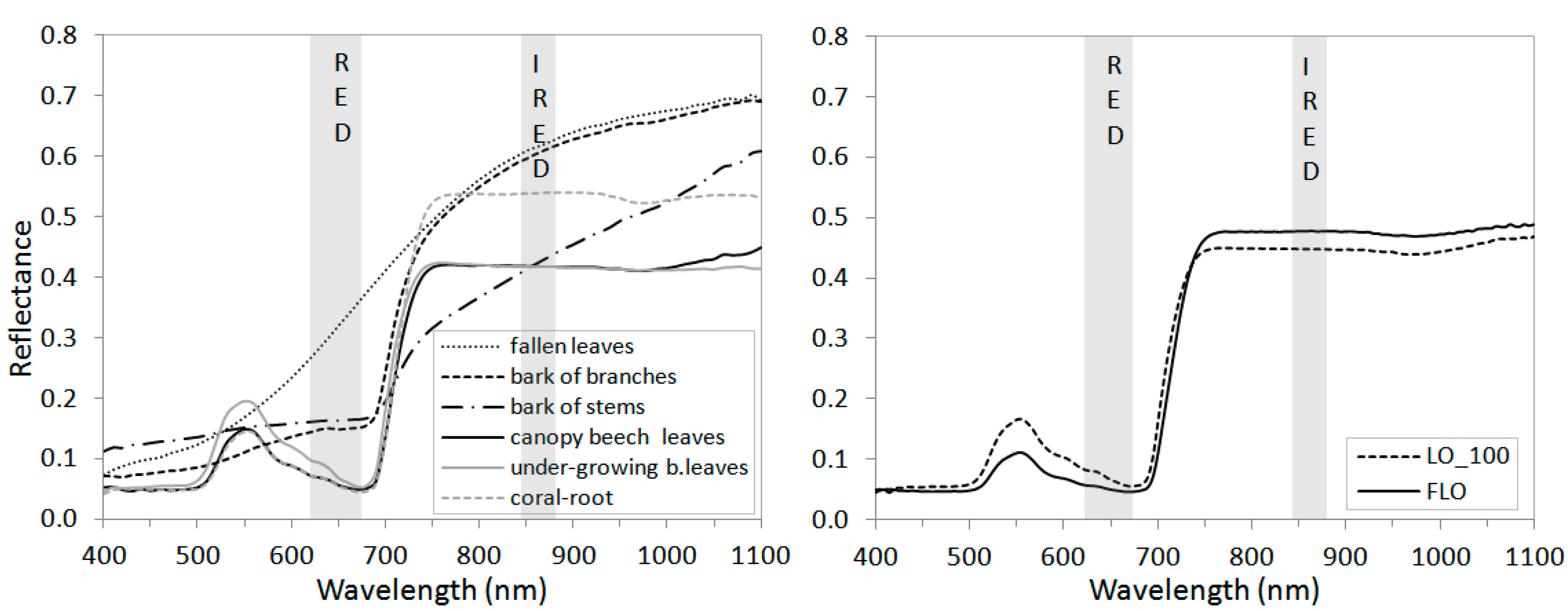
In the laboratory, we analyzed the spectral reflectance of beech leaves fallen in the previous growing season which covered the ground in beech stands before the beginning of the growing season. The NDVILAB of the fallen leaves was lower than the satellite data-based NDVIMOD (Table 3). This suggested the presence of other forest components enhancing NDVIMOD at this time. Analyses revealed that a bark from beech trees reflected the considerable amount of the red and near infrared radiation (Figure 3a). It was interesting to find the differences between the NDVILAB sampled from the bark of the branches and NDVILAB of the bark from the stems (Table 3). These parts of trees are visible for satellites through the canopies up to the end of leaf onset (LO_100). The spectral analyses of the collected samples of green leaves revealed that the NDVILAB of the leaves from the under-growing beech trees was lower than the NDVILAB of the beech leaves from the canopy (Table 3). The spectral reflectance of these leaves differ in the red spectra (Figure 3a). Next, at the time of LO_100, the NDVILAB of the canopy beech leaves was lower than the NDVILAB at the time of final leaf onset (Table 3). This stemmed from the differences in spectral reflectance which at LO_100 was higher in the red spectrum (RED) and lower in the near-infrared spectrum (IRED) than at FLO (Figure 3b). The beech leaves collected when these two phenological phases started differed in their color, size, and structure (Figure 4).
Based on data from the laboratory spectral analyses and in situ observations, it was concluded that the low values of NDVIMOD from the time with no green vegetation in the beech-dominated stands was caused together by presence of fallen leaves and the above-ground parts of the trees. This state lasted until DOY 93, when the NDVIMOD was 0.45 on average.
The slight increase of the NDVIMOD after DOY 98 caused flushing of the spring heliophytes—coral-root and dog’s mercury. NDVILAB of them reached 0.71 and 0.70 for coral-root and dog’s mercury, respectively, and they covered from 5% (stands U1, U2, U4, U5) to 14% (stand U3) of the forest floor (Table S1). Subsequently, following the spring heliophytes, the under-growing beeches started their phenological phases. The NDVIMOD was around 0.58 (Table 3) when the canopy green leaves finished only the bud bursting (BB_100). The beech trees from the understory ended the leaf onset around DOY 110, when the cover of the ground vegetation in study stands was from 7 to 20% (Table S1). The most rapid increase of NDVIMOD was recorded from 0.58 (DOY 110) to 0.87 (DOY 124) from the end of canopy beech bud bursting to the end of leaf onset (from BB_100 to LO_100). After LO_100, both the NDVIMOD and NDVILAB showed the continuing development of the canopy beech leaves. This development was also captured by the hemispherical photography, when the LAI values increased after LO_100 (Figure 5).
The maximum values of NDVIMOD equal to 0.93 were achieved on DOY 146. At this time, the period of spring phenological phases of the canopy beech trees finished. The foliage was fully developed and this was the time of the final leaf onset. The maximum LAI values of the growing season were observed on DOY 170, but could appear earlier between the measurements on DOY 133 and 170. After reaching the final leaf onset, NDVIMOD started to slowly decrease. This gradual decrease from the average NDVIMOD of 0.93 to 0.86 lasted until DOY260.
The beginning of leaf coloring (LC_10) was observed on DOY 270. From this time, the NDVIMOD started to decrease faster, and this reduction was also recorded by the hemispherical images (Figure 5). After the leaf fall started on average on DOY 290, the decreasing LAI captured this loss of leaves in the canopy. The NDVIMOD continued decreasing and when the general leaf coloring (LC_50) was reached around DOY 290, the average NDVIMOD value was 0.76. Over the next two weeks, the NDVIMOD dropped to 0.54. The last NDVIMOD value recorded on DOY 319 was 0.52. At that time, all leaves were discolored and the NDVIMOD represented the reflectance of the forest components without green leaves and vegetation–litter, above-ground parts of trees, and brown leaves lasting on branches.
3.2. Assigning the Phenological Metrics to the In Situ Observed Phenological Phases
The phenological metrics were assigned to the in situ observed phenological phases according to the closest onset day and the differences were tested. In the first step of validation, the phenological data from the twelve study stands and the single years were compared against the corresponding data from phenological metrics. If the validations could not be realized due to the missing phenological phases that were not observed in the phenological network of the Slovak Hydrometeorological Institute, we validated only the phenological data from the detailed phenological observations from stands U1–U5.
3.2.1. Spring Phenological Phases
- In situ observed phenological phases such as bud swelling and bud bursting were not possible to observe in the satellite data because the increasing NDVIMOD at the time of their occurrence was caused by other forest components, and not by the canopy beech leaves. Therefore, phenological metric S1 was not paired with any in situ observed phenological phases.
- Phenological metric S2 was assigned to the beginning of leaf onset (LO_10). The paired sample t-test revealed non-significant differences between S2 and LO_10 (t = 0.03 < T0.01(90) = 1.96). The correlation coefficient indicated very strong correlation between LO_10 and S2 (Figure 6). The average NDVIMOD of the S2 was 0.67.
- Phenological metric S3 was assigned to the phenological phase LO_50, and although the r = 0.84 (Figure 6) suggested a very strong correlation between S3 and LO_50, the t-test revealed significant differences with a RMSE of 6.24. The phenological metric S3 was overestimated. The phenological data from the SHMI, which were the base data for the validation, did not contain information on the phenological phase LO_100, which, according to our detailed phenological monitoring, occurred on average four days after LO_50. No significant differences were revealed between S3 and LO_100 (t = 0.10 < T0.01(9) = 3.25) in our U1–U5 stands, although the correlation coefficient was smaller than the one between S3 and LO_50 (Figure 6). A control test by adding four days (average difference between LO_50 and LO_100) to the days of LO_50 from the SHMI observations was performed. The differences between the estimated LO_100 and S3 were non-significant (t = 0.54 < T0.01(90) = 1.96) with the RMSE of 4.57. The average NDVIMOD of S3 was 0.81.
3.2.2. Autumn Phenological Phases
- Phenological metric A1 occurred between the two autumn phenological phases: beginning of leaf coloring (LC_10) and general leaf coloring (LC_50), on average eight days after LC_10. Thus, we paired A1 with LC_10 and LC_50 from all twelve study stands and single years, but the differences in both cases were significant. Then, using data from detailed phenological monitoring on the U1–U5 stands, the pairs of A1 with LC_20, LC_30, and LC_40 were tested, but the differences in all of the tested pairs were significant.
- The paired test of the onset days of A2 and LC_50 revealed an average time lag of 13 days for the A2 phenological metric. Based on that, the pairs of A2 with LC_60, LC_70, LC_80, LC_90, and LC_100 recorded in the U1–U5 stands were tested. Only the paired t-test with LC_80 revealed non-significant differences (t = 1.51 < T0.01(9) = 3.25) between the in situ LC_80 and satellite data-based A2.
- A3 occurred after the end of leaf coloring (LC_100) when only the understory vegetation was green, but the beech trees had no green leaves. Therefore, this phenological metric was not paired with any autumn in situ observed phenological phase.
- The correlation between the onset days of the autumn phenological phases and phenological metrics was weak, with the correlation coefficient not exceeding 0.30 (Figure 7).
3.3. Phenological Metrics along the Altitudinal Gradient
Phenological metrics validated in the previous sections were used in the large-scale analyses of the effect of altitude on the onset days of phenological phases. We evaluated the phenological metrics S2, S3, A2, and GSL corresponding to the phenological phases beginning of leaf onset, end of leaf onset, 80% leaf coloring, and the growing season length, respectively. The representative onset dates of a particular phenological phase expressed by the phenological metrics were calculated for each beech-dominated pixel from the beech mask and averaged over a temporal series of 13 years (2000–2012). In all cases, the large-scale regression analyses revealed non-linear dependences of the phenological metrics on altitude. The second order polynomial function was used to fit the datasets (Figure 8a–d). The altitudinal gradients derived from regression functions are shown in Table 4.
The average beginning of leaf onset expressed by the S2 metric increased with altitude. At low altitudes (200–300 m a.s.l.), the beginning of leaf onset occurred earliest on DOY 108 and delayed with the increasing altitude up to DOY 141 (Figure 8a). Strong dependence was revealed between S2 and altitude, since 68% of the total variation in the onset days of S2 was caused by their dependence on the altitude. The difference between the earliest and the latest S2 days estimated from the regression function was 33 days.
The polynomial function, which characterized the altitudinal gradient of average end of leaf onset expressed by the S3 (Figure 8b), had a very similar course to the one for S2 with a 31-day difference between the earliest onset at lowest altitudes (DOY 118) and the latest onset of S3 at the highest altitudes (DOY 150). Dependence of S3 on the altitude was strong, as 72% of the total variation in the onset days of S3 could be explained by the applied second order polynomial function.
The altitudinal gradient of the average onset days of 80% leaf coloring, expressed by the phenological metric A2, differed from those of the spring phenological phases. The latest onset of A2 was generally revealed in the altitudinal range of 400–600 m a.s.l. Only a weak relationship was found between A2 and altitude as the polynomial function could explain only 6% of the A2 variation. According to our datasets, the variability in the onset of this autumn phenological phase was greater in the comparison with leaf onset. In particular, in the altitudinal range 300–700 m a.s.l., an unexpected very early onset of A2 from DOY 270 in more pixels was recorded (Figure 8c).
The length of the growing season was quite varying from 127 days at the highest altitudes to 188 days at the lowest altitudes. Using the second order polynomial function, 27% of the total variation in the growing season length of beech pixels by its dependence on altitude could be explained. Used regression function indicated that the differences in growing season length in the altitudinal range from 156 to 500 m a.s.l. varied within two days and was shortened with increasing altitude.
When considering only the phenological metrics from our 12 study stands, the regression analyses revealed that a linear function fit the data better. The changes at a stand scale estimated by the linear regression along the altitudinal gradient were smaller than those revealed at a large-scale. The S2 of stands delayed by two days at 100 m−1 and S3 delayed by 2.8 days at 100 m−1. The onset of S3 along the altitudinal gradient changed a little bit more gradually than that of S2. The onset of A2 derived from the regression model advanced only 0.8 days at 100 m−1 and GSL was shortened by about 2.5 days at 100 m−1.
The average GSL of the 12 study stands was considered from the climatic aspect using the normal temperatures and precipitation. The longest growing season (188–193 days) with the early onset of LO_10 (S2) and the latest LC_80 (A2) was at the lowest altitudes <500 m a.s.l. (Table S2). The stands situated from 500 to 700 m a.s.l. had the GSL between 181–185 days. The shortest growing seasons (170–174 days) with the latest LO_10 (S2) were found in the stands located at the highest altitudes >1000 m a.s.l. (Table S2). The normal temperature of stands increased linearly with altitude by 0.61 °C for every 100 m increase in altitude. The R2 = 0.97 indicated a very strong correlation between altitude and normal temperature (Figure S1). The absolute difference of normal temperature between the beech stands at the lowest and the highest altitude was 4.9 °C. The length of the growing season extended along the temperature gradient by 4.5 days for every 1 °C of normal temperature increase and a very strong relationship between these two variables was found (Figure 9a). The rate of change in the normal precipitation with increasing altitude was 28 mm with 100 m of the lift. Study stands are situated in moderate moist to moist climatic areas and the absolute difference in precipitation between the beech stands at the lowest and the highest altitude was only 188 mm. The relationship between altitude and precipitation was strong with R2 = 0.77 (Figure S1). GSL shortened by −6.9 days with every 100 mm of precipitation increase. The relationship between GSL and normal of precipitation expressed by R2 was 0.55 (Figure 9b).
4. Discussion
The results presented in this study were based on the daily MODIS products called MOD09 and MYD09, which had good capability of detecting gradual changes in green leaves at the time of leaf onset and to date it accurately. Derived single-pixel NDVIMOD values represented the reflectance of all forest components. The effect of different forest components on the satellite data-based vegetation indices had already been outlined in previous studies. Reed et al. [16] pointed out that the reflectance at every pixel was the conglomeration of a variety of vegetation and background features, which may obscure observations of initial bud burst. During spring, the understory generally starts earlier than the main tree species. Testa et al. [17] found out that when the understory in beech stands reached the 90% level of leaf onset, the main species had only reached its 10% level. These tendencies were also revealed in our beech study stands and raised questions about what is hidden behind the NDVI value of the beech forests, especially at the time before the canopy closing. The laboratory spectral analyses revealed that not only did the leaves of the understory and canopy participate in the pixel reflectance, but other parts of trees also reflected the red and near-infrared radiation important for the NDVI calculation. The chlorophyll content in the bark of beech stems and branches [47] absorbed a considerable amount of radiation in the red spectra. This resulted in NDVILAB values similar to that of the fallen leaves (Figure 3). The presence of fallen leaves, stems, and branches in the beech pixels kept the NDVIMOD on a relatively stable level (around 0.42) when there was no snow cover on the forest floor. NDVIMOD started to increase from that level after the incidence of the first spring heliophytes and the undergrowth flushing, but the canopy beech trees were only in the phenological phase of 10% bud bursting, and therefore had no green leaves. The reflectance signal of bud burst was not sufficient to alter the reflectance signal from a larger mixed pixel, while field observers may be able to note bud swelling and bursting [13,14]. With regard to previous studies [8,17,48,49,50], it is probable that the incidence of spring heliophytes and the undergrowth strategy of phenological escape is a common occurrence in forests. Therefore, the first phenological metric occurring simultaneously with the beginning of the bud bursting of the canopy (BB_10), usually situated at the beginning of NDVI increase on the sigmoid function (in this study phenological metric S1), characterized the leafing of the understory and thus was not suitable to track phenological phases of the canopy trees. Liang et al. [14], who assigned the first point on the NDVI sigmoid function (S1) to the end of bud bursting (BB_100) of the canopy trees, revealed an underestimation of S1 of more than two weeks. In most cases, this point on the NDVI profile could be interpreted as a start of the vegetation period in forests in general [12], but not as a tree specific phenological phase. Different results may be obtained when the enhanced vegetation index (EVI) is used to track the phenological phases because of its insensitivity to the forest background. Significant agreement was found between the first point on the EVI piecewise sigmoid function and BB_10 [14]. According to these results, we concluded that the pairing of phenological metrics from EVI and NDVI fitted with the in situ observed phenological phases needed two different approaches. However, MODIS spectral bands needed for EVI calculations were available from the spatial resolution 500 m, we preferred to analyze NDVI time series calculated from the bands available from the resolution 250 m.
The variables derived from the in situ observations provided information that could be used for the interpretation of the variables derived from the satellite data. The leaf area index is one of the main variables affecting the vegetation reflectance and is also an indicator of changing phenological phases. The LAI measurements were used to analyze the phenological changes, especially after the leaf onset and during the autumn leaf coloring and leaf fall. The analyses of NDVIMOD seasonal profiles revealed a continuous increase after the in situ observed end of leaf onset (DOY124), similar to the findings with EVI [13]. Our findings were supported by the measurements of the LAI and NDVILAB of the beech leaf samples. NDVILAB increased from 0.71 on DOY 127 to 0.79 on DOY 159. This increase was caused by the increased reflectance in the near-infrared spectrum and decreased reflectance in the red spectrum related to the increasing chlorophyll content between LO_100 and final leaf onset (FLO) [51]. In FLO, the leaves achieved their final shape, size, and structure, which were also recognized by the LAI measurements based on hemispherical photography. At that time, the foliage was fully developed. FLO is visually hardly observable because of the minimal structural changes of canopy leaves that are barely visible to the human eye, but is recordable by optical and spectral measurement based indices. Subsequently, after reaching the maximum leaf area, the LAI and NDVIMOD started to slightly decrease. Similar results have been revealed in beech and oak stands in France, where the NDVI, measured by an in situ downward looking spectroradiometer, recorded a slight monotonic decrease during the spring period [52,53]. In the summer months, there is no biosynthesis of the chlorophyll in beech leaves, thus the photo-degraded chlorophyll is not replaced by the new [54]. This phenomenon of NDVI decrease measured at the leaf-level was marked as “summer greendown”, to which NDVI is sensitive [51]. The reduction of LAI during the summer period can be explained by a drop of turgor in the leaf cells due to the lack of moisture. In autumn, the indices reacted to the different phenological phases. While the decreasing LAI was caused by the ongoing leaf fall, the NDVI reflected the changes in leaf color and structure.
The next step in the validation process was to assign the satellite data-based phenological metrics to the ground observed phenological phases. The key problem in pairing these two data sources presented by previous authors was the insufficient frequency of the ground phenological observations, resulting in greater differences between the paired values [9]. In this study, very detailed phenological monitoring was performed to exclude this deficiency, and significant matches were found. According to our results, the first spring vegetative phenological phase that could be reliably deduced from the NDVIMOD phenology metrics used in this study was the LO_10 of canopy beech trees, which corresponded to S2 (inflection point) with a bias of 0 days and an average NDVIMOD of 0.67. The phenological phase LO_10 was observed, on average, three days after full bud bursting, which is usually paired with the inflection point of the NDVI sigmoid function (S2) [48,55]. Nevertheless, Fisher and Mustard [9] also revealed that the inflection point of the sigmoid function occurred between the observed BB_50 and LO_50, closer to LO_50. In this study, the next spring phenological phase LO_100 was linked to S3, with an average NDVIMOD equal to 0.81. The NDVIMOD values of S2 and S3 corresponded to those measured in the field spectral experiment published by Nagai et al. [50], who concluded that NDVI of 0.6 indicated the start of leaf expansion, a NDVI of 0.7 indicated that about 50% of the canopy leaves had expanded, and a NDVI of 0.8 meant that all of the canopy leaves had expanded.
Determination of the autumn phenological phases from the metrics used in this study was more complicated when compared to the spring phenological phases. The main reason for this is the development of the European beech phenological phases, especially the order of beech leaves coloring. The phenological phase of the autumn senescence of beech leaves start from the upper and edge parts of the canopy [56]. These leaves are directly exposed to sunlight and photodegrade first. The satellite data scan forests from above and thus are able to record these first changes of leaf senescence, while the in situ observers, looking from the ground concurrently, do not recognize any progress. Hence, there is a question of which beginning of leaf coloring is more reliable as they do not appear to be comparable. In this study, A1 was paired with different stages of observed leaf coloring and no matches were found, although this phenological metric appeared between the observed LC_10 and LC_50. For further validation of the first autumn phenological metric, we proposed the use of cameras placed above the canopy [57] or drones [58], which could identify the phenological phases from the same direction as the satellites. The next phenological metric, A2, which is commonly used in other studies to identify leaf senescence, was the inflection point of the sigmoid function. Some other authors have marked this point as the beginning of yellowing [58] or paired it with the leaf fall phase [15,50,59]. This phenological metric (A2) appeared after LC_50 was observed in all of the study stands. Using the data from the detailed monitoring in U1–U5, it was compared to all phenological stages of leaf coloring observed after LC_50. Significant agreement was found with LC_80. The last point on the sigmoid function, A3, occurred after LC_100 and therefore was not interpreted in relation to the beech phenological phases. In a coarser context, it could be interpreted as the beginning of dormancy in these stands. Liu et al. [60] marked the last point as the full leaf coloring with differences of 0–12 days, but also concluded that the MODIS VI data consistently estimated later dormancy onset relative to the ground observed full leaf coloration. In this study, the leaf fall phenological phase was not evaluated using NDVIMOD based phenological metrics because it is related to the position of leaves, and not their reflectance.
Altitude is the most significant factor when considering the effect of topography on the onset of phenological phases, and it is linked with the reduction of air temperature and increase of precipitation [61]. Averaging the phenological metrics from 13 years into a single representative value made it possible to investigate the altitude variations in seasonal remote sensing responses over a large range of altitudes (from 156 to 1331 m a.s.l.). Regression analyses were utilized to discover the dependence of the onset of European beech phenological phases on the altitude and climatic conditions. The analyses were performed at two levels: at the stand scale and at a large-scale, which demonstrated different results. While the stand scale regressions revealed linear relationships with correlations (R2) of 0.92, 0.88, 0.26, and 0.88 for S2, S3, A2, and GSL, respectively, the large-scale analyses found non-linear regressions between the phenology and altitude. In previous studies, linear regression trends have been demonstrated in stand scale analyses, which were similar to our results. The studies discovered a lag of 1.1 days 100 m−1 with R2 = 0.63 (10 stands, France) [43], and a lag of 1 day 100 m−1 with R2 = 0.51 (22 stands, France) [4] in the oceanic climate of Western Europe; a lag of 2.6 days 100 m−1 with R2 = 0.73 in the south of Central Europe (47 stands, Slovenia) [42]; and a lag of 1.7–3.9 days 100 m−1 with R2 = 0.22–0.81 to the west of Central Europe (97 stands divided into six regions, Germany) [41]. In the above-mentioned studies, regression analyses of the onset of the autumn coloring of European beech revealed only a weak dependence on altitude with a R2 less than 0.20 [41,42].
Missing the ground observed data in the highest altitude could lead into the linear dependence of the spring phenological phases on altitude. The study stands observed in situ are located in the ecological optimum or suboptimum of the distributional range of European beech, where the effect of the temperature could be dominant. In the highest altitudes, where the ecological pessimum for growing occurs, the phenology onset reflects the interaction of extreme ecological conditions such as lower temperature; longer snow cover; stronger winds, etc. The trees in such conditions react by the much later onset of leafing, bringing the non-linearity in the shape of regression. When a large amount of data along the whole altitudinal gradient is available, the regression curve may acquire a variety of shapes. Hwang et al. [61] applied a non-linear model fitting procedure to derive the local patterns of topography-mediated vegetation phenology from MODIS vegetation indices. Except for midday of the green-up period, all variables showed quadratic associations with altitude, reflecting an interaction between the topoclimatic patterns of temperature and water availability. Gyon et al. [4] used linear regression for the leaf onset days along the altitudinal gradient, but the results revealed that for low altitudes (<500 m a.s.l.), the delay of leaf onset was less than the expected one: 1.5 days 100 m−1 compared to 2.3 days 100 m−1 when applied to the whole altitudinal range. The second order polynomial function best fitted our phenological data in relation to altitude. When comparing the spring and autumn phases, the onset days of the S2 and S3 metrics were less variable, with the data concentrated around the approximated value.
The onset of LC_80 had already started in some beech forests at the end of the summer. This early onset may result from a variety of causes. One source of discrepancies could be the lack of NDVIMOD data, hence, the distorted fitting procedure. This may appear during the autumn months, when the incidence of fog and low clouds is more probable in the mountainous landscape. The next cause of a decline in NDVIMOD could be due to some kind of leaf damage. During the growing season, beech trees and leaves are threatened by several biotic (insects) and abiotic (hot temperatures, drought stress, incidence of spring and summer frost, etc.) factors, and trees could also be harvested in the managed forests. Regardless of these anomalies, the onsets of the autumn phenological phases were very variable and only partially depended on the altitude.
The capability of detecting altitude-mediated phenology offers the potential to detect vegetation responses to local-climate conditions. In this study, we used the normal values of temperature and precipitation from the last 30 years to assess the altitude-conditioned differences in growing season length at the study stand scale. The rate of temperature change along the altitudinal gradient (0.61 °C 100 m−1) corresponded with the generally valid moist adiabatic lapse rate. The temperature conditions with a sufficient amount of precipitation ensured the longest growing season (188–193 days) at the lowest altitudes (<500 m a.s.l.). This is related to both the early beginning of leaf onset LO_10 and the late onset of 80% leaf coloring (LC_80). However, the temperature and precipitation conditions seemed to be the most suitable for European beech growth; the beech trees at these altitudes could be most endangered by the late frost damage [62,63]. Fresh new leaves are especially vulnerable. The average length of the growing season in the stands situated from 500 to 700 m a.s.l. varied between 181–185 days. Here, the normal precipitation differed only slightly between the study stands, while the temperature decrease resulted in shorter growing seasons with both later onset of LO_10 and the earlier onset of LC_80 in comparison to stands at the lowest altitudes. The shortest growing seasons (170–174 days) were found in the stands located at the highest altitudes (>1000 m a.s.l.). The lowest temperature in the moist environment lead to the late onset of LO_10, but the end of the growing season in these climate conditions appeared on similar days as at the lower altitudes. From the point of beech production, this is an important finding since canopy duration affects the carbon assimilation rates and the energy budget of forest ecosystems from the stand-level to the global scale [64]. It has been proven that the length of the growing season correlates with tree height and diameter growth while this effect is associated with the timing of growth cessation rather than with leaf onset [65]. It follows that beech stands at higher altitudes are similarly productive as those situated lower, while the probability of late frost damage is much smaller. When the sensitivity of leaf onset days to temperature from our study were compared with the data from Western Europe, there was a much lower sensitivity of European beech to temperature decrease (−2.1 days °C−1) in Western Europe [43]. The differences in the sensitivity of leaf onset days to temperature between the data from Western (France) and Central Europe (Slovakia) may result from the genetically conditioned internal periodicity of different populations of European beech. Furthermore, the data from the west of Central Europe (Germany) showed differences in the sensitivity of the beech growing season length on altitude-conditioned climatic factors and population locations [41]. The onset of phenological phases and growing season length could vary around the presented averaged data with regard to other climatic or topographic factors, which were not considered in this study.
5. Conclusions
The remote sensing-based approaches for monitoring phenology have been the focus of research over the past decades. The validation of the phenological metrics against the in situ observation data is still crucial. Here, the data retrieved from the in situ phenological observations, detailed monitoring of the forest stands, laboratory spectral analyses, and LAI measurements were used to detect what the satellite data represent. Next, we described and tested a method to detect the timing of spring and autumn phenological phases for beech-dominated stands. Our results show that phenological metrics applied here correspond closely to phenological observations collected on the ground in 12 beech-dominated stands. Significant compliance was found especially in the spring period. The onset of autumn phenological phases needs to be further explored due to the observation discrepancy between downward looking satellites and upward looking observers. In the future, the utilization of phenological cameras or drones could fill the gaps in the data validation.
The phenological metrics we described in this paper have the potential to improve the knowledge of phenological responses to a variety of factors. The large-scale altitudinal study presented here showed the advantage of validated satellite data-based phenological metrics. However, the moderate spatial resolution data source MODIS was used, so the results suggest that it should be possible to generate multi-year observations of phenological phases at 250 m spatial resolution over large areas. The large-scale analysis can provide new opportunities to study tree-species phenology in the context of climate change.
Supplementary Materials
The following are available online at https://www.mdpi.com/1999-4907/10/1/60/s1, Figure S1: The relationship between altitude and normal temperature and precipitation on the study stands, Table S1: Average cover of ground vegetation in stands U1–U5, Table S2: Average transition days of the phenological metrics S2 and A2, and the growing season length, with the temperature and precipitation normal.
Author Contributions
V.L., J.Š. (Jaroslav Škvarenina), and J.Š. (Jana Škvareninová) conceived and designed the experiments; V.L. and J.Š. (Jana Škvareninová) performed the experiments; V.L. and T.B. analyzed the data; T.B. and J.Š. (Jaroslav Škvarenina) contributed reagents/materials/analysis tools; and V.L. wrote the paper.
Acknowledgments
This work was accomplished as part of the VEGA projects No.: 1/0589/15, 1/0111/18 and 1/0500/19 of the Ministry of Education, Science, Research, and Sport of the Slovak Republic and the Slovak Academy of Science; and the projects of the Slovak Research and Development Agency No.: APVV-15-0425 and APVV-15-0497. The authors thank these agencies for their support. The authors are notably thankful to two researchers: Ing. Ivana Vasiľová and Ing. Jozef Zverko for their participation in detailed phenological monitoring; and to Ing. Vladimír Kriššák for his technical support during the terrestrial works.
Conflicts of Interest
The authors declare no conflict of interest. The founding sponsors had no role in the design of the study; in the collection, analyses, or interpretation of data, in the writing of the manuscript, and in the decision to publish the results.
References
- Ciais, P.; Sabine, C.; Bala, G.; Bopp, L.; Brovkin, V.; Canadell, J.; Chhabra, A.; DeFries, R.; Galloway, J.; Heimann, M.; et al. Carbon and Other Biogeochemical Cycles. In Climate Change 2013: The Physical Science Basis. Contribution of Working Group I to the Fifth Assessment Report of the Intergovernmental Panel on Climate Change; Stocker, T.F., Qin, D., Plattner, G.-K., Tignor, M., Allen, S.K., Boschung, J., Nauels, A., Xia, Y., Bex, V., Midgley, P.M., Eds.; Cambridge University Press: Cambridge, UK; New York, NY, USA, 2013; pp. 465–570. [Google Scholar] [CrossRef]
- Badeck, F.W.; Bondeau, A.; Böttcher, K.; Doktor, D.; Lucht, W.; Schaber, J.; Sitch, S. Responses of spring phenology to climate change. New Phytol. 2004, 162, 295–309. [Google Scholar] [CrossRef] [Green Version]
- Polgar, C.; Gallinat, A.; Primack, R.B. Drivers of leaf-out phenology and their implications for species invasions: Insights from Thoreau’s Concord. New Phytol. 2014, 202, 106–115. [Google Scholar] [CrossRef]
- Guyon, D.; Guillot, M.; Vitasse, Y.; Cardot, H.; Hagolle, O.; Delzon, S.; Wigneron, J.P. Monitoring elevation variations in leaf phenology of deciduous broadleaf forests from SPOT/VEGETATION time-series. Remote Sens. Environ. 2011, 115, 615–627. [Google Scholar] [CrossRef]
- Mátyás, C.; Berki, I.; Czúcz, B.; Gálos, B.; Móricz, N.; Rastovits, E. Future of Beech in Southeast Europe from the Perspective of Evolutionary Ecology. Acta Silv. Lignaria Hung. 2010, 6, 91–110. [Google Scholar]
- Becker, M. Taxonomie et characteres botaniques. In Le Hetre; Teissier du Cros, E., Ed.; INRA: Paris, France, 1981; pp. 35–49. ISBN 978-2-7592-0512-7. [Google Scholar]
- Myneni, R.B.; Hoffman, S.; Knyazikhin, Y.; Privette, J.L.; Glassy, J.; Tian, Y.; Wang, Y.; Song, X.; Zhang, Y.; Smith, G.R.; et al. Global products of vegetation leaf area and fraction absorbed PAR from year one of MODIS data. Remote Sens. Environ. 2002, 83, 214–231. [Google Scholar] [CrossRef] [Green Version]
- Fisher, J.I.; Mustard, J.F.; Vadeboncoeur, M.A. Green leaf phenology at Landsat resolution: Scaling from the field to the satelite. Remote Sens. Environ. 2006, 100, 265–279. [Google Scholar] [CrossRef]
- Fisher, J.I.; Mustard, J.F. Cross-scalar satellite phenology from ground, Landsat and MODIS data. Remote Sens. Environ. 2007, 109, 261–273. [Google Scholar] [CrossRef]
- Beck, P.S.A.; Atzberger, C.; Høgda, K.A.; Johansen, B.; Skidmore, A.K. Improved monitoring of vegetation dynamics at very high latitudes: A new method using MODIS NDVI. Remote Sens. Environ. 2006, 100, 321–334. [Google Scholar] [CrossRef]
- Jönsson, A.M.; Hellström, M.; Bärring, L.; Jönsson, P. Annual changes in MODIS vegetation indices of Swedish coniferous forests in relation to snow dynamics and tree phenology. Remote Sens. Environ. 2010, 114, 2719–2730. [Google Scholar] [CrossRef]
- Zhang, X.; Friedl, M.A.; Schaaf, C.B.; Strahler, A.H.; Hodges, J.C.F.; Gao, F.; Reed, B.C.; Heute, A. Monitoring vegetation phenology using MODIS. Remote Sens. Environ. 2003, 84, 471–475. [Google Scholar] [CrossRef]
- White, K.; Pontius, J.; Schaberg, P. Remote sensing of spring phenology in northeastern forests: A comparison of methods, field metrics and sources of uncertainty. Remote Sens. Environ. 2014, 148, 97–107. [Google Scholar] [CrossRef]
- Liang, L.; Schwartz, M.D.; Fei, S. Validating satellite phenology through intensive ground observation and landscape scaling in a mixed seasonal forest. Remote Sens. Environ. 2011, 115, 143–157. [Google Scholar] [CrossRef]
- Chen, X.; Luo, X.; Xu, L. Comparison of spatial patterns of satellite-derived and ground-based phenology for the deciduous broadleaf forest of China. Remote Sens. Lett. 2013, 4, 532–541. [Google Scholar] [CrossRef]
- Reed, B.C.; Brown, J.F.; VanderZee, R.; Merchant, J.W.; Ohlen, D.O. Measuring phenological variability from satellite imagery. Int. Assoc. Veg. Sci. 1994, 5, 703–714. [Google Scholar] [CrossRef]
- Testa, S.; Soudani, K.; Boschetti, L.; Borgogno Mondino, E. MODIS-derived EVI, NDVI and WDRVI time series to estimate phenological metrics in French deciduous forests. Int. J. Appl. Earth Obs. Geoinf. 2018, 64, 132–144. [Google Scholar] [CrossRef]
- Škvarerninová, J.; Snopková, Z. The Development of Phenological Stages of European Beach (Fagus sylvatica L.) in Slovakia During the Period of 1996–2010. In Proceedings of the Bioclimate: Source and Limit of Social Development, Topoľčianky, Slovakia, 6–9 September 2011; pp. 87–90. [Google Scholar]
- Škvareninová, J. Vplyv Zmeny Klimatických Podmienok na Fenologickú Odozvu Ekosystémov; Vydavateľstvo Technickej Univerzity vo Zvolene: Zvolen, Slovakia, 2013; 132p, ISBN 978-80-228-2598-6. [Google Scholar]
- Bucha, T. Classification of tree species composition in Slovakia from satellite images as a part of monitoring forest ecosystems biodiversity. Acta Inst. For. Zvolen 1999, 9, 65–84. [Google Scholar]
- Meier, U. Growth Stages of Mono- and Dicotyledonous Plants, 2nd ed.; Federal Biological Research Centre for Agriculture and Forestry: Berlin, Germany; Braunschweig, Germany, 2001; 158p. [Google Scholar]
- Bruns, E.; Chmielewski, F.M.; van Vliet, A.J.H. The Global Phenological Monitoring Concept. In Phenology: An Integrative Environmental Science; Schwartz, M., Ed.; Springer: Dordrecht, The Netherlands, 2003; pp. 93–104. ISBN 978-94-007-0632-3. [Google Scholar]
- Chmielewski, F.M.; Rötzer, T. Phenological trends in Europe in relation to climatic changes. Agrometeorol. Schr. 2000, 7, 1–15. [Google Scholar]
- Škvareninová, J.; Tuhárska, M.; Škvarenina, J.; Babálová, D.; Slobodníková, L.; Slobodník, B.; Středová, H.; Minďaš, J. Effects of light pollution on tree phenology in the urban environment. Morav. Geogr. Rep. 2017, 25, 282–290. [Google Scholar] [CrossRef] [Green Version]
- Babálová, D.; Škvareninová, J.; Fazekaš, J.; Vyskot, I. The dynamics of the phenological development of four woody species in south-west and central Slovakia. Sustainability 2018, 10, 1497. [Google Scholar] [CrossRef]
- Lukasova, V.; Lang, M.; Skvarenina, J. Seasonal changes in NDVI in relation to phenological phases, LAI and PAI of beech forests. Balt. For. 2014, 20, 248–262. [Google Scholar]
- Land Processes Distributed Active Archive Center. Available online: https://lpdaac.usgs.gov/dataset_discovery/modis/modis_products_table/mod09gq_v006 (accessed on 13 March 2018).
- Ju, J.; Roy, D.P.; Shuai, Y.; Schaaf, C. Development of an approach for generation of temporally complete daily nadir MODIS reflectance time series. Remote Sens. Environ. 2011, 114, 1–20. [Google Scholar] [CrossRef]
- Franch, B.; Vermote, E.F.; Sobrino, J.A.; Fédèle, E. Analysis of directional effect on atmospheric correction. Remote Sens. Environ. 2013, 128, 276–288. [Google Scholar] [CrossRef]
- Townshend, J.R.G.; Huang, S.N.; Kalluri, V.; Defries, R.S.; Liang, S. Beware of the per-pixel characterization of land cover. Int. J. Remote Sens. 2000, 21, 839–843. [Google Scholar] [CrossRef]
- Bucha, T.; Koreň, M. Phenology of the beech forests in the Western Carpathians from MODIS for 2000–2015. iForest Biogeosci. For. 2017, 10, 537–546. [Google Scholar] [CrossRef]
- Evans, J.D. Straightforward Statistics for the Behavioral Sciences; Brooks/Cole Publishing: Pacific Grove, CA, USA, 1996; 600p. [Google Scholar]
- Kramer, K. Phenotypic plasticity of the phenology of seven European tree species in relation to climatic warming. Plant Cell Environ. 1995, 18, 93–104. [Google Scholar] [CrossRef]
- Matsumoto, K.; Ohta, T.; Irasawa, M.; Nakamura, T. Climate change and extension of the Ginkgo biloba L. growing season in Japan. Glob. Chang. Biol. 2003, 9, 1634–1642. [Google Scholar] [CrossRef]
- Estrella, N.; Menzel, A. Response of leaf colouring in four deciduous tree species to climate and weather in Germany. Clim. Res. 2006, 32, 253–267. [Google Scholar] [CrossRef]
- Wang, T.; Ottle, C.; Peng, S.; Janssens, I.A.; Lin, X.; Poulter, B.; Yue, C.; Ciais, P. The influence of local spring temperature variation on temperature sensitivity of spring phenology. Global Chang. Biol. 2014, 20, 1473–1480. [Google Scholar] [CrossRef]
- Koike, T. Autumn coloring, photosynthetic performance and leaf development of deciduous broad-leaved trees in relation to forest succession. Tree Physiol. 1990, 7, 21–32. [Google Scholar] [CrossRef]
- Lee, D.W.; O’Keefe, J.; Holbrook, N.M.; Feild, T.S. Pigment dynamics and autumn leaf senescence in a New England deciduous forest, eastern USA. Ecol. Res. 2003, 18, 677–694. [Google Scholar] [CrossRef]
- Menzel, A. Phenology: Its importance to the global change community. Clim. Chang. 2002, 54, 379–385. [Google Scholar] [CrossRef]
- Broich, M.; Huete, A.; Tulbure, M.G.; Ma, X.; Xin, Q.; Paget, M.; Restrepo-Coupe, N.; Davies, K.; Devadas, R.; Held, A. Land surface phenological response to decadal climate variability across Australia using satellite remote sensing. BioGeoSci. Discuss. 2014, 11, 7685–7719. [Google Scholar] [CrossRef]
- Dittmar, C.; Elling, W. Phenological phases of common beech (Fagus sylvatica L.) and their dependence on region and altitude in Southern Germany. Eur. J. Forest Res. 2006, 125, 181–188. [Google Scholar] [CrossRef]
- Čufar, K.; Luis, M.D.; Saz, M.A.; Črepinšek, Z.; Kajfež-Bogataj, L. Temporal shifts in leaf phenology of beech (Fagus sylvatica) depend on elevation. Trees 2012, 26, 1091–1100. [Google Scholar] [CrossRef]
- Vitasse, Y.; Delzon, S.; Dufrene, E.; Pontiller, J.Y.; Louvet, J.M.; Kremer, A.; Michalet, R. Leaf phenology sensitivity to temperature in European trees: Do within-species populations exhibit similar responses? Agric. Forest Meteorol. 2009, 149, 735–744. [Google Scholar] [CrossRef]
- Dunn, A.H.; Beurs, K.M. Land surface phenology of North American mountain environments using moderate resolution imaging spectroradiometer data. Remote Sens. Environ. 2011, 115, 1220–1233. [Google Scholar] [CrossRef]
- Ahrens, C.D.; Henson, R. Meteorology today: An Introduction to Weather, Climate, and the Environment, 11th ed.; Cengage Learning: Boston, MA, USA, 2015; 656p, ISBN 978-1-305-26500-4. [Google Scholar]
- Climatic Conditions of Slovak Republic. Available online: http://www.shmu.sk/sk/?page=1064 (accessed on 12 March 2018).
- Pfanz, H.; Aschan, G. The Existence of Bark and Stem Photosynthesis in Woody Plants and Its Significance for the Overall Carbon Gain. An Eco-Physiological and Ecological Approach. In Progress in Botany; Springer: Berlin, Germany, 2001; Volume 62, pp. 477–510. [Google Scholar] [CrossRef]
- Richardson, A.D.; O’Keefe, J. Phenological differences between understory and overstory: A case study using the long-therm Harvard forest records. In Phenology of Ecosystem Processes; Noormets, A., Ed.; Springer: New York, NY, USA, 2009; pp. 88–117. [Google Scholar] [CrossRef]
- Ahl, D.E.; Gower, S.T.; Burrows, S.N.; Shabanov, N.V.; Myneni, R.B.; Knyazikhin, Y. Monitoring spring canopy phenology of a deciduous broadleaf forest using MODIS. Remote Sens. Environ. 2006, 104, 88–95. [Google Scholar] [CrossRef] [Green Version]
- Nagai, S.; Nasahara, K.N.; Muraoka, H.; Akiyama, T.; Tsuchida, S. Field experiments to test the use of the normalized-difference vegetation index for phenology detection. Agric. Forest Meteorol. 2010, 150, 152–160. [Google Scholar] [CrossRef] [Green Version]
- Yang, X.; Tang, J.; Mustard, J.F. Beyond leaf color: Comparing camera-based phenological metrics with leaf biochemical, biophysical, and spectral properties throughout the growing season of a temperate deciduous forest. J. Geophys. Res. Biogeosci. 2014, 119, 181–191. [Google Scholar] [CrossRef] [Green Version]
- Soudani, K.; Hmimina, G.; Delpierre, N.; Pontailler, J.Y.; Aubinet, M.; Bonal, D.; Caquet, B.; de Grandcourt, A.; Burban, B.; Flechard, C.; et al. Ground-based Network of NDVI measurements for tracking temporal dynamics of canopy structure and vegetation phenology in different biomes. Remote Sens. Environ. 2012, 123, 234–245. [Google Scholar] [CrossRef]
- Hmimina, G.; Dufrêne, E.; Pontailler, J.Y.; Delpierre, N.; Aubinet, M.; Caquet, B.; de Grandcourt, A.; Burban, B.; Flechard, C.; Granier, A.; et al. Evaluation of the potential of MODIS satellite data to predict vegetation phenology in different biomes: An investigation using ground-based NDVI measurements. Remote Sens. Environ. 2013, 132, 145–158. [Google Scholar] [CrossRef]
- García-Plazaola, J.I.; Becerril, J.M. Seasonal changes in photosynthetic pigments and antioxidants in beech (Fagus sylvatica) in a Mediterranean climate: Implications for tree decline diagnosis. Aust. J. Plant Physiol. 2001, 28, 225–232. [Google Scholar] [CrossRef]
- Soudani, K.; Maire, G.; Dufrêne, E.; François, C.H.; Delpierre, N.; Ulrich, E.; Cecchini, S. Evaluation of the onset of green-up in temperate deciduous broadleaf forests derived from Moderate Resolution Imaging Spectroradiometer (MODIS) data. Remote Sens. Environ. 2008, 112, 2643–2655. [Google Scholar] [CrossRef]
- Chalupa, V. Počátek, trvání a ukončení vegetační činnosti u lesních dřevin. Práce VÚLHM 1969, 37, 41–68. [Google Scholar]
- Toda, M.; Richardson, A.D. Estimation of plant area index and phenological transition dates from digital repeat photography and radiometric approaches in a hardwood forest in the Northeastern United States. Agric. Forest Meteorol. 2018, 249, 457–466. [Google Scholar] [CrossRef]
- Klosterman, S.; Richardson, A.D. Observing spring and fall phenology in a deciduous forest with aerial drone imagery. Sensors 2017, 17, 2852. [Google Scholar] [CrossRef]
- Nagai, S.; Inoue, T.; Ohtsuka, T.; Kobayashi, H.; Kurumado, K.; Muraoka, H.; Nasahara, K.N. Relationship between spatio-temporal characteristics of leaf-fall phenology and seasonal variations in near surface- and satellite-observed vegetation indices in cool-temperate deciduous broad-leaved forest in Japan. Int. J. Remote Sens. 2014, 35, 3520–3536. [Google Scholar] [CrossRef]
- Liu, L.; Liang, L.; Schwartz, M.D.; Donnelly, A.; Wang, Z.; Schaaf, C.B. Evaluating the potential of MODIS satellite data to track temporal dynamics of autumn phenology in a temperate mixed forest. Remote Sens. Environ. 2015, 160, 156–165. [Google Scholar] [CrossRef]
- Hwang, T.; Song, C.; Vose, J.M. Topography-mediated controls on local vegetation phenology estimated from MODIS vegetation index. Landsc. Ecol. 2011, 26, 541–556. [Google Scholar] [CrossRef]
- Dittmar, C.; Fricke, W.; Elling, W. Impact of late frost events on radial growth of common beech (Fagus sylvatica L.) in Southern Germany. Eur. J. Forest Res. 2006, 125, 249–259. [Google Scholar] [CrossRef]
- Kreyling, J.; Thiel, D.; Nagy, L.; Jentsch, A.; Huber, G.; Konnert, M.; Beierkuhnlein, C. Late frost sensitivity of juvenile Fagus sylvatica L. differs between southern Germany and Bulgaria and depends on preceding air temperature. Eur. J. Forest Res. 2012, 131, 717–725. [Google Scholar] [CrossRef]
- Kindermann, J.; Wurth, G.; Kohlmaier, G.H.; Badeck, F.W. Interannual variation of carbon exchange fluxes in terrestrial ecosystems. Global Biogeochem. Cycles 1996, 10, 737–755. [Google Scholar] [CrossRef]
- Gomory, D.; Paule, L. Trade-of between height growth and spring flushing in common beech (Fagus sylvatica L.). Ann. Forest Sci. 2011, 68, 975–984. [Google Scholar] [CrossRef]
Figure 1.
Map of the beech stands with the presence of European beech at 60% and higher (grey color). The locations of the study stands with in situ phenological observations are marked with red crosses.
Figure 1.
Map of the beech stands with the presence of European beech at 60% and higher (grey color). The locations of the study stands with in situ phenological observations are marked with red crosses.

Figure 2.
Graphical illustration of NDVIMOD seasonal profile fitted by a sigmoid logistic function with the inflection points of the first derivative (phenological metrics S2 and A2), and the local minima and maxima of the second derivative (phenological metrics S1, S3 and A1, A3 for the spring and autumn period, respectively). NDVI, normalized difference vegetation index. DOY, day of year.

Figure 3.
Spectral reflectance of all beech forest components measured with a Li 1800 integration sphere (a) and beech leaves from the phenological phases LO_100 (end of leaf onset) and final leaf onset (FLO) (b). The grey columns marked RED and IRED highlight the wavelengths used in the NDVILAB calculations.

Figure 4.
Difference in the beech leaves between the phenological phases of full leaf onset LO_100 (a) and final leaf onset (FLO) (b).
Figure 4.
Difference in the beech leaves between the phenological phases of full leaf onset LO_100 (a) and final leaf onset (FLO) (b).

Figure 5.
Seasonal changes in the NDVIMOD and LAI averaged over the test stands of U1–U5 in 2011. The year was divided into sections according to the phenological phases of canopy beech trees. NDVI_MOD, normalized difference vegetation index from MODIS data, LAI, leaf area index. DOY, day of year. BB_100, end of bud bursting. LO_100, end of leaf onset. LC_10, beginning of leaf coloring. LC_50, general leaf coloring. LC_100, end of leaf coloring.

Figure 6.
Correlation between the in situ observed spring phenological phases and assigned spring phenological metrics: S2 and beginning of leaf onset LO_10 (a), S3 and general leaf onset LO_50 (b), S3 and end of leaf onset LO_100 (c). The high values of the correlation coefficient indicated very strong correlation between the phenological phases and phenological metrics. DOY, day of year.

Figure 7.
Correlation between the in situ observed autumn phenological phases and assigned autumn phenological metrics: A1 and beginning of leaf coloring LC_10 (a), A2 and general leaf coloring LC_50 (b), A2 and 80% leaf coloring LC_80 (c). The correlation was weak in all cases. DOY, day of year.
Figure 7.
Correlation between the in situ observed autumn phenological phases and assigned autumn phenological metrics: A1 and beginning of leaf coloring LC_10 (a), A2 and general leaf coloring LC_50 (b), A2 and 80% leaf coloring LC_80 (c). The correlation was weak in all cases. DOY, day of year.

Figure 8.
Satellite-based phenological metrics S2 (a), S3 (b), A2 (c), and growing season length, GSL (d) as a function of altitude at a stand-level and large-scale level. The individual phenological metrics of 12 study stands are indicated by red triangles and the altitudinal trend is the linear red line. The phenological metrics derived from all beech-dominated stands (60% of beech and higher) in the area of Slovakia are indicated by black crosses and the altitude trend is the polynomial blue line. DOY, day of year.

Figure 9.
Growing season length in the twelve study stands in relation with normal temperature (a) and precipitation (b).
Figure 9.
Growing season length in the twelve study stands in relation with normal temperature (a) and precipitation (b).


Table 1.
The basic characteristics of beech study stands.
| Stand Number | Identifier | Altitude | Aspect | Presence of Beech (%) | Climatic Region | Climate Normal (1981–2010) | |
|---|---|---|---|---|---|---|---|
| T 7 (°C) | P 8 (mm) | ||||||
| 1 | ZS | 304 | NW | 60 | W7 1 | 10.1 | 675 |
| 2 | MY | 457 | W | 65 | M3 2 | 9 | 729 |
| 3 | U1 | 490 | W | 85 | M6 3 | 8.6 | 691 |
| 4 | U5 | 512 | N | 70 | M3 | 8.3 | 700 |
| 5 | U2 | 522 | W | 65 | M6 | 8.3 | 700 |
| 6 | ZV | 566 | SW | 65 | M6 | 8 | 745 |
| 7 | KC | 570 | SW | 90 | M3 | 8.1 | 644 |
| 8 | MU | 579 | N | 100 | M7 4 | 7.9 | 689 |
| 9 | U4 | 607 | E | 100 | M6 | 7.8 | 760 |
| 10 | U3 | 615 | W | 65 | M6 | 7.8 | 760 |
| 11 | CS | 1003 | N | 90 | C1 5 | 5.2 | 857 |
| 12 | PO | 1051 | SE | 80 | C2 6 | 5.7 | 863 |
1 Warm, moderate moist with mild winters, 2 Moderate warm, moderate moist, upland to highland, 3 Moderate warm, moist, highland, 4 Moderate warm, very moist, highland, 5 Moderate cold, 6 Cold mountain, 7 Temperature, 8 Precipitation.
Table 2.
Definition of the phenological phases observed in all study stands.
| Phenological Phase | BBCH Codes | Definition |
|---|---|---|
| Beginning of Bud Bursting (BB_10) | BBCH07 | When bud scales opened and green top of leaf was sticking out |
| Beginning of Leaf Onset (LO_10) | BBCH11 | When 10% of leaves have final shape, but not final size and color |
| General Leaf Onset (LO_50) | BBCH13 | When 50% of leaves have final shape, but not final size and color |
| Beginning of Leaf Coloring (LC_10) | - | When 10% of leaves changed their color from green to yellow, red or brown |
| General Leaf Coloring (LC_50) | BBCH94 | When 50% of leaves changed their color from green to yellow, red or brown |
| Beginning of Leaf Fall (LF_10) | BBCH93 | When 10% of leaves fell down from trees to the ground |
| End of Leaf Fall (LF_100) | BBCH97 | When 100% of leaves fell down from trees to the ground |
Table 3.
NDVILAB of the samples collected on the particular DOY and the satellite-based NDVIMOD derived tor the same DOY: mean ± standard deviation, and the number of samples and values respectively, in the brackets.
Table 3.
NDVILAB of the samples collected on the particular DOY and the satellite-based NDVIMOD derived tor the same DOY: mean ± standard deviation, and the number of samples and values respectively, in the brackets.
| Time of Sampling–DOY | 97 | 110 | 127 | 159 |
|---|---|---|---|---|
| Date | 7.4 | 20.4 | 7.5 | 8.6 |
| Canopy beech leaves | - | - | 0.71 ± 0.023 (10) | 0.79 ± 0.015 (8) |
| Under-growing beech leaves | - | - | 0.66 ± 0.011 (15) | - |
| Fallen leaves | 0.34 ± 0.067 (8) | - | - | |
| Bark of branches | - | - | - | 0.63 ± 0.028 (5) |
| Bark of stems | - | - | - | 0.46 ± 0.042 (14) |
| Coral-root | - | 0.71 ± 0.012 (4) | - | - |
| Dogs mercury | - | 0.70 ± 0.003 (3) | - | - |
| NDVIMOD | 0.48 ± 0.062 (7) | 0.58 ± 0.017 (10) | 0.87 ± 0.010 (10) | 0.91 ± 0.008 (5) |
Table 4.
The altitudinal gradient of the phenological metrics S2, S3, A2, and GSL calculated from regression functions for each 100 m of the vertical distribution range of beech-dominated pixels (from 156 to 1331 m a.s.l.). Values in the table were rounded to the whole day.
Table 4.
The altitudinal gradient of the phenological metrics S2, S3, A2, and GSL calculated from regression functions for each 100 m of the vertical distribution range of beech-dominated pixels (from 156 to 1331 m a.s.l.). Values in the table were rounded to the whole day.
| Altitude | Altitudinal Gradient of Large-Scale Phenology | Difference on Altitudinal Gradient | ||||||
|---|---|---|---|---|---|---|---|---|
| S2 | S3 | A2 | GSL | S2 1 | S3 1 | A2 2 | GSL 3 | |
| 156 | 109 | 118 | 296 | 186 | 0 | - | −3 | −2 |
| 200 | 108 | 118 | 296 | 187 | 0 | 0 | −2 | −1 |
| 300 | 108 | 119 | 298 | 188 | - | 1 | −1 | - |
| 400 | 109 | 120 | 299 | 187 | 0 | 2 | 0 | 0 |
| 500 | 110 | 122 | 299 | 186 | 1 | 3 | - | −2 |
| 600 | 111 | 124 | 298 | 183 | 3 | 5 | 0 | −4 |
| 700 | 113 | 126 | 297 | 179 | 5 | 8 | −1 | −8 |
| 800 | 116 | 129 | 296 | 174 | 8 | 10 | −3 | −13 |
| 900 | 120 | 132 | 293 | 168 | 11 | 13 | −5 | −20 |
| 1000 | 124 | 135 | 291 | 161 | 15 | 17 | −8 | −27 |
| 1100 | 128 | 139 | 287 | 152 | 20 | 21 | −12 | −36 |
| 1200 | 133 | 143 | 283 | 142 | 25 | 25 | −16 | −45 |
| 1300 | 139 | 148 | 279 | 131 | 31 | 30 | −20 | −57 |
| 1331 | 141 | 150 | 277 | 127 | 33 | 31 | −22 | −60 |
1 Differences from the earliest onset of S2 and S3, respectively, 2 Differences from the latest onset of A2, 3 Differences from the longest growing season.
© 2019 by the authors. Licensee MDPI, Basel, Switzerland. This article is an open access article distributed under the terms and conditions of the Creative Commons Attribution (CC BY) license (http://creativecommons.org/licenses/by/4.0/).
Share and Cite
MDPI and ACS Style
Lukasová, V.; Bucha, T.; Škvareninová, J.; Škvarenina, J. Validation and Application of European Beech Phenological Metrics Derived from MODIS Data along an Altitudinal Gradient. Forests 2019, 10, 60. https://doi.org/10.3390/f10010060
AMA Style
Lukasová V, Bucha T, Škvareninová J, Škvarenina J. Validation and Application of European Beech Phenological Metrics Derived from MODIS Data along an Altitudinal Gradient. Forests. 2019; 10(1):60. https://doi.org/10.3390/f10010060
Chicago/Turabian StyleLukasová, Veronika, Tomáš Bucha, Jana Škvareninová, and Jaroslav Škvarenina. 2019. "Validation and Application of European Beech Phenological Metrics Derived from MODIS Data along an Altitudinal Gradient" Forests 10, no. 1: 60. https://doi.org/10.3390/f10010060
Note that from the first issue of 2016, this journal uses article numbers instead of page numbers. See further details here.