Article

The Potential of Multisource Remote Sensing for Mapping the Biomass of a Degraded Amazonian Forest

1
CIRAD, Forêts et Sociétés, F-34398 Montpellier, France
2
Forêts et Sociétés, University Montpellier, CIRAD, 34398 Montpellier, France
3
LISAH, University Montpellier, INRA, IRD, Montpellier SupAgro, 34398 Montpellier, France
4
Department SIAFEE AgroParisTech, 75231 Paris, France
5
Environmental Change Institute, University of Oxford, Oxford OX1 3QY, UK
6
Lancaster Environment Centre, Lancaster University, Lancaster LA1 4YQ, UK
7
UMR CNRS LETG 6554, Laboratory of Geography and Remote Sensing COSTEL, Université de Rennes 2, 35043 Rennes, France
8
Centre de Recherche et de Documentations sur les Amériques (CREDA), UMR 7227, Université Sorbonne Nouvelle, Paris 3, 75006 Paris, France
9
UMR CNRS ESO (Espaces et Sociétés), Le Mans Université, 72000 Le Mans, France
*
Author to whom correspondence should be addressed.
Forests 2018, 9(6), 303; https://doi.org/10.3390/f9060303
Submission received: 13 April 2018 / Revised: 24 May 2018 / Accepted: 25 May 2018 / Published: 29 May 2018

Abstract

:
In the agricultural frontiers of Brazil, the distinction between forested and deforested lands traditionally used to map the state of the Amazon does not reflect the reality of the forest situation. A whole gradient exists for these forests, spanning from well conserved to severely degraded. For decision makers, there is an urgent need to better characterize the status of the forest resource at the regional scale. Until now, few studies have been carried out on the potential of multisource, freely accessible remote sensing for modelling and mapping degraded forest structural parameters such as aboveground biomass (AGB). The aim of this article is to address that gap and to evaluate the potential of optical (Landsat, MODIS) and radar (ALOS-1 PALSAR, Sentinel-1) remote sensing sources in modelling and mapping forest AGB in the old pioneer front of Paragominas municipality (Para state). We derived a wide range of vegetation and textural indices and combined them with in situ collected AGB data into a random forest regression model to predict AGB at a resolution of 20 m. The model explained 28% of the variance with a root mean square error of 97.1 Mg·ha−1 and captured all spatial variability. We identified Landsat spectral unmixing and mid-infrared indicators to be the most robust indicators with the highest explanatory power. AGB mapping reveals that 87% of forest is degraded, with illegal logging activities, impacted forest edges and other spatial distribution of AGB that are not captured with pantropical datasets. We validated this map with a field-based forest degradation typology built on canopy height and structure observations. We conclude that the modelling framework developed here combined with high-resolution vegetation status indicators can help improve the management of degraded forests at the regional scale.

1. Introduction

Deforestation and forest degradation are major sources of greenhouse gas emissions [1,2], contributing to forest carbon losses [3], global climate change, affecting biodiversity [4] and the entire forest ecosystem. While deforestation refers to the rapid conversion from forest to non-forest areas, degradation implies changes in the forest structure with no change in land use [5,6]. In Amazonia, over the last decades, deforestation and forest degradation have shaped the rural landscape, resulting in a complex mosaic of fragmented forests associated with agricultural lands [7]. A total area of 766,448.5 km2 was cleared in 2015 [8], representing 20% of Amazonia [9,10].
Since 2005, deforestation in Brazil has drastically decreased thanks to coercive measures taken by the Brazilian government associated with private initiatives (soy and beef moratoria), among other factors [11]. However, these measures are not effective for reducing forest degradation [12,13]. Most of the remaining forested lands are degraded due to the accumulation over time and space of severe degradation processes mainly triggered by anthropogenic impacts through unsustainable logging practices, fire, shifting cultivation and charcoal production [14,15].
Reducing forest degradation is a major challenge given the rapid need to reduce carbon emissions to the atmosphere, conserve biodiversity, limit soil erosion and regulate the water cycle [16]. Forest monitoring based on the forest/non-forest approach used to quantify deforestation is not relevant for providing information on the forest status [17,18]. The biomass value of a forest is a relevant indicator to quantify the intensity of degradation [19]. Forest biomass mapping is therefore a critical step to reach the challenge [20].
At the pantropical scale, two maps of biomass density that present the spatial distribution of the biomass of all forest types at a moderate resolution [21,22] have been used as baselines for the tropical belt. More recently, a harmonized reference aboveground biomass (AGB) map has been released that significantly improves the estimation and local distribution of AGB using the combination of in-situ collected data, remote sensing and regional biomass maps [23].
At the local scale, most of the approaches integrate field-collected data with Light Detection and Ranging (LIDAR) to scale up forest biomass natural distribution, which normally requires spatial interpolation of in-situ biomass [24]. LIDAR can map the forest canopy in three dimensions and can retrieve accurate forest biomass through forest canopy height and structure [25,26,27,28,29]. It is also sensitive to the carbon density of the different types of degraded forests, from logging at a low impact to forest stands burned multiple times [30]. Satellite LIDAR has been used in validating AGB maps [31], calibrating local regressions between in situ AGB data and metrics derived from LIDAR footprints and extrapolating using different remote sensing sources [28,32]. However, most airborne and satellite LIDAR datasets are often difficult to access (acquisition cost) and to replicate in both time and space [33].
At the meso-scale (regional), many studies demonstrated the potential of optical and radar remote sensing-derived indicators to characterize degraded forests [34]. The study of degraded forests requires the analysis of vertical and horizontal disturbances within the forest structure [5,33,35,36,37]. Optical images can provide information on the photosynthetic activity and moisture of the forest canopy [38]. Spectral unmixing approaches are recognized to be the most effective method to assess the status of degraded forests using the percentage of active vegetation, dead vegetation and bare soil at the pixel scale [15,39,40]. Radar images are sensitive to the texture of the impacted forest canopy [41]. Canopy texture-derived indicators based on co-occurrence matrices use the variance of the signal in a given window to spatially quantify the distribution of tree crowns structure [42,43,44]. Estimating the biomass from the radar data generally concerns wavelengths up to the meter (band P or L) with signal saturation thresholds around 200 Mg/ha of AGB [45,46,47].
This review of recent remote sensing methods illustrates the trade-off that needs to be made between resolution, accuracy, area covered, cost and frequency to map forest biomass. It also highlights the fact that there is remarkably little information at the regional scale on the potential of open access optical and radar remote sensing to model and map the aboveground biomass of degraded forests. Most of the approaches tend to capture the local variation of AGB following environmental variables, i.e., climate, topography and natural forest dynamic gradients, but do not particularly capture the distribution along anthropogenic disturbance gradients [30].
In this sense, there is a need to better understand how remotely sensed indicators perform with AGB modelling at the regional scale in order to provide relevant information to decision makers on the state of the resource of remnants forest.
In order to answer this need, this paper aims (i) to assess the potential of multisource, multi-indicator and open access remote sensing in modelling and mapping aboveground biomass of degraded forests; (ii) to quantify the spatial distribution of degraded forest biomass in comparison with the pantropical AGB map; and (iii) to evaluate the relevance of this regional forest AGB mapping at the stand scale.
This quantification is highly informative for forested land use planning and policy makers. Many South American governments and global NGOs are seeking more accurate and definitive information about the scale of degradation so they can propose policies and actions to ameliorate and reduce the level of degradation [48].

2. Materials and Methods
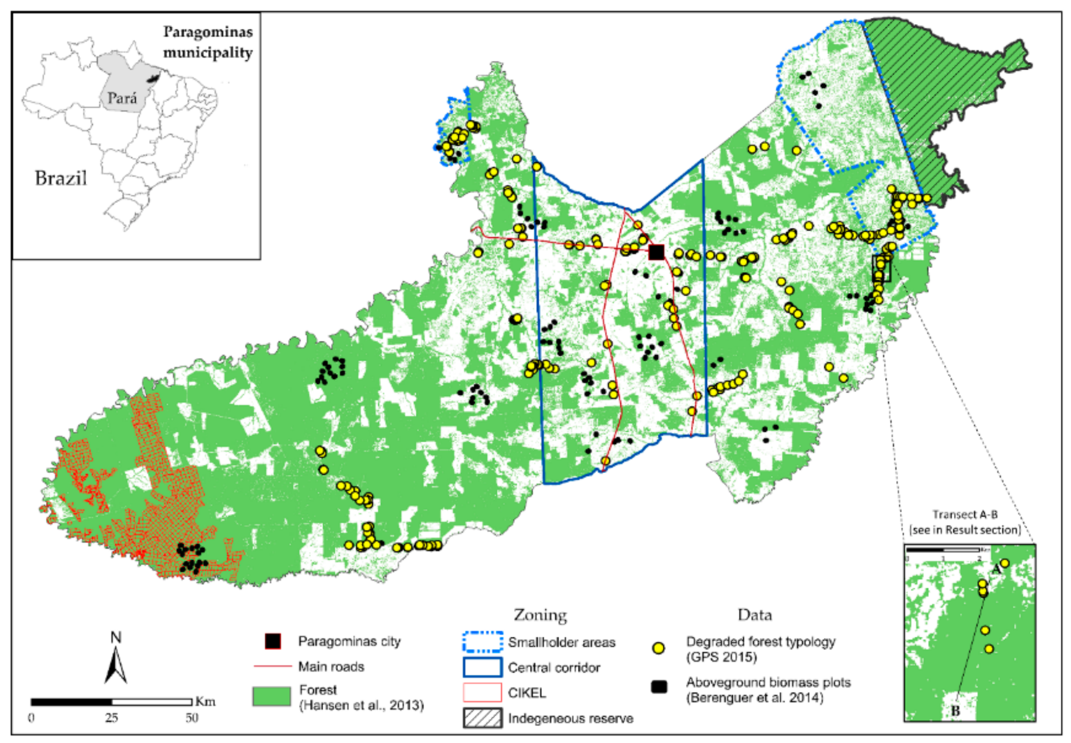
2.1. Study Area

The study was carried out in the municipality of Paragominas, located in the northeastern part of the State of Para, Brazil, and covering an area of 19,342 km2 with a population size of 108,547 [49]. The municipality was founded in 1965 along the BR-010 road connecting Brasilia to Belém (Figure 1). The colonization process led to a large conversion of lands into pasture, with cattle ranching becoming the dominant land use. The municipality went through a succession of different economical models that have drastically shaped the landscape [50]. The boom in the logging industry started from the 1980s, where most of the timber was transformed in the 350 sawmills located along the main road. Deforestation and forest degradation were accentuated with the grain agribusiness boom in the 2000s (soybean and maize cultivation) and charcoal production. In 2007, the municipality was red-listed by the federal government as one of the most deforested Amazonian municipalities. The consequences were an immediate loss of access to credit and market for any commodities. Many charcoal plants and illegal sawmills were shut down. In response to this governmental ban, Paragominas became the first “green municipality” in the country in 2008 in order to end illegal deforestation, to tend to zero net deforestation by 2014, and to promote alternative production systems and reforestation. Land management was also improved through the Rural Environmental Registry [51].

2.2. In Situ AGB Collection

Aboveground biomass data were collected during the dry seasons in 2009 and 2010 by teams from the Sustainable Amazon Network (Rede Sustentavel Amazonia—RAS) [19,52,53]. In total, 18 study sites were randomly selected in the municipality of Paragominas. For each site, plots of 250 m by 20 m were designed, resulting in a total of 121 plots. Each plot represents a homogeneous type of forest, classified into four types: undisturbed forest, logged forest, logged forest and burned and secondary forest. Aboveground biomass was estimated using Chave’s allometric equations [54] and was based on the measurements and identification of all live trees, palms and lianas (≥10 cm DBH). The results of this study showed significant differences in biomass for each type of forest (Table 1). We chose a threshold of 286 Mg·ha−1 to distinguish between degraded and sustainably managed or conserved forests. Mazzei et al. [55] showed that undisturbed forests store on average 409.8 Mg·ha−1 in the Cikel Fazenda, located in the western part of the municipality (Figure 1). The mean AGB total lost under reduced-impact logging operations is 94.5 Mg·ha−1, which represents around 23% of biomass lost [55]. The threshold is thus the percentage of biomass lost applied to the undisturbed primary forest biomass identified by RAS.
The aboveground vegetation that corresponds to the largest carbon storage compartment is very sensitive to the type of disturbance, with about a 40% of difference in ABG between mature forests and secondary forests. We used the RAS AGB dataset in shapefile format to calibrate the Random Forest model presented in Section 2.4.

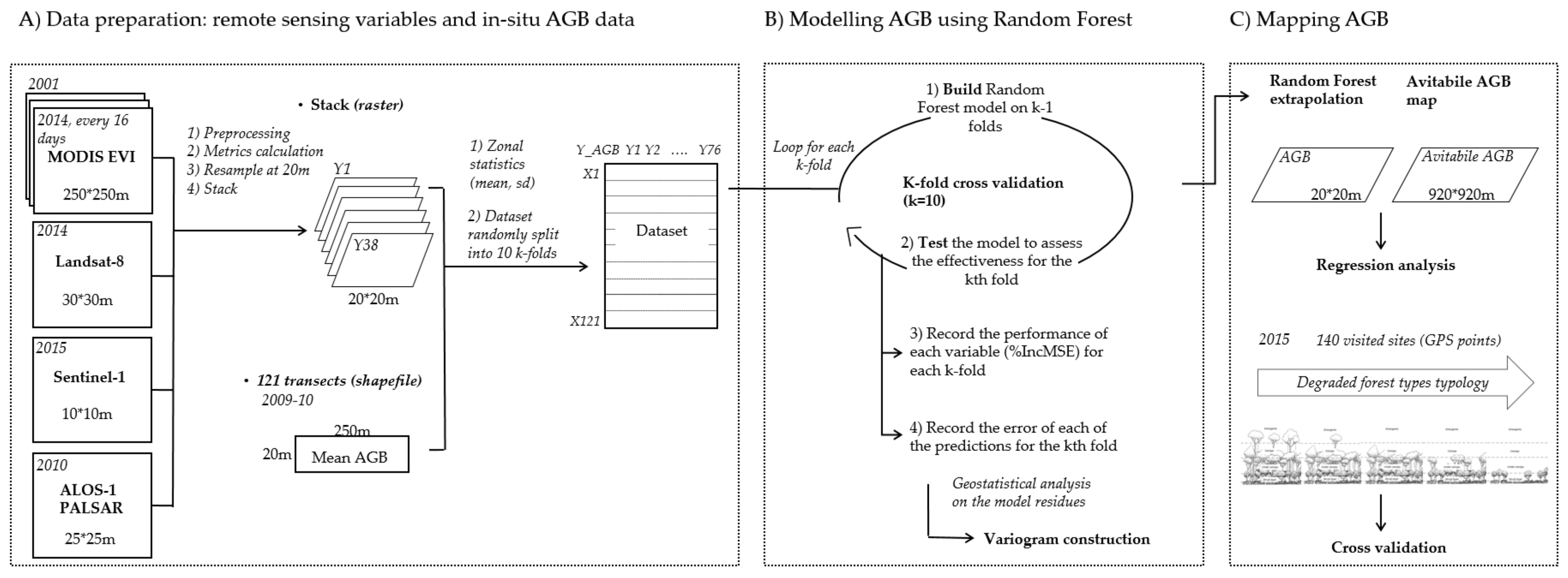
2.3. Remote Sensing Multisource Data: Image Acquisition, Pre-Processing and Biophysical Indicators Variables Extraction

We used 38 indicators derived from passive (MODIS, Landsat-8) and active (ALOS-1, Sentinel-1) remote sensing sources. These indicators are correlated with different vegetation parameters such as photosynthesis activity and vegetation structure. All the satellite images used in this study are freely available and span the globe.
• MODIS
To quantify forest canopy health and temporal dynamics, we used the enhanced vegetation index (EVI) from the MODIS sensor. EVI was extracted from the ‘16-Day L3 Global 250m product (MOD13Q1 c5)’ from January 2001 to December 2014. EVI is directly related to photosynthetic activity [56]. It does not saturate quickly for high values of chlorophyll activity and provides improved sensitivity for high biomass areas such as tropical forests [38]. The 16-day composite was built by choosing within the 16 daily acquisitions the two pixels with the highest value of NDVI (Normalized Difference Vegetation Index). Of these two values, the pixel with the smallest viewing angle was chosen in order to minimize the residual angle [56]. A quality filter was then applied to the composite to remove clouds and reduce atmospheric contamination [38]. We extracted three indicators from this dataset: the mean and the standard deviation calculated for the whole time series based on annual average EVI and the pooled variance which is the weighted sum of annual variance based on the number of values available for each pixel for each year (giving more weight to the pixels that were not under cloud coverage during the 16 days × 14-year period).
Pooled   variance = i = 1 14 V a r i a n c e ( i ) × a v a i l a b l e   v a l u e s ( i ) i = 1 14 a v a i l a b l e   v a l u e s ( i ) 14
These three indicators provide global information on the stability of the forest canopy photosynthetic activity.
• Landsat 8
We used three Landsat 8 images taken during the dry season of 2014, at 30 m resolution. We acquired the surface reflectance data with the pre-processing already performed with the algorithm developed by the NASA Goddard Space Flight Center (GSFC). We used 5 spectral bands (blue, green, red, near-infrared and short-wave infrared) and we derived 13 indicators using the Orfeo toolbox [57]. We used the Carnegie Landsat Analysis System-lite (Claslite) to derive the Photosynthetic Vegetation (PV), Non Photosynthetic Vegetation (NPV) and Bare Soil indexes [39].
• ALOS-1 PALSAR
We downloaded seven images ALOS-1 PALSAR (L-band) taken in 2010 from the JAXA (Japan Aerospace Agency, http://www.eorc.jaxa.jp/ALOS/en/index.htm) platform. These images have 25-m spatial resolution (“ALOS-1 mosaic 25 m” product) and are dual-polarized (HH and HV). The incidence angle varies between 35° (near range) to 42° (far range). The images were correctly geo-referenced, so we only processed the conversion from digital raw number (DN) to gamma and sigma following these two equations [58,59]:
gamma   [ dB ] = 10 × l o g 10 ( D N ² ) 83
sigma   [ dB ] = 10 × l o g 10 ( D N ² ) 83 + 10 × l o g 10 ( c o s θ )
We tested these two indicators, expecting a strong correlation between backscatter coefficients and aboveground biomass [47].
• Sentinel-1
We acquired one image Sentinel-1 (C-band, dual polarization VV/VH, descending pass direction) taken in May 2015, at 10-m resolution and in Interferometric Wide (IW) swath mode. We performed the pre-processing using the free software Sentinel Toolbox, which allows the derivation of backscatter coefficients and processing of the range Doppler terrain corrections using the 3 arc-seconds SRTM Digital Elevation Model. We derived 9 indicators from the grey level co-occurrence matrix (GLCM) that are based on the statistical relationship between the values of the pixels within a 9 × 9 pixels window [60]. These indicators are relevant to quantify forest canopy texture [61].
The source, description of the remote sensing images and the derived indicators are detailed in the Appendix A, Table A1.

2.4. Random Forest Regression Model

We used a random forest regression tree to explore the performance of the different remote sensing data sources and derived indicators for AGB modelling and mapping. Regression trees are particularly efficient for remotely sensed indicators that show unknown multivariate patterns and nonlinear relationships [62].

2.4.1. Data Preparation

We resampled the indicators at 20-m resolution using GRASS libraries and stacked them all together to make sure they are georeferenced in the same system. This resolution matches with the size of the plot measurements. For each indicator, we generated an automatic process to extract the mean and standard deviation within the extent of each plot. We then compiled all the data in a file with the identification of each plot (row 1 to 121) and the estimated AGB followed by the mean and standard deviation of the 38 indicators (columns). Finally, this dataset is randomly mixed to avoid any biases related to its original structure and is split into 10 folds (Figure 2). This number of folds (k) is often suggested in order to balance bias limitation (lower value of k) and variability (higher value of k) [63].

2.4.2. Modelling AGB with Random Forest

For each independent indicator, regression trees recurrently split the data into more homogeneous samples and identify the most significant indicator that gives best homogeneous sets of samples [64]. Random Forest grows multiple trees (500 trees in our study) by randomization of data subsampling in order to improve the predictive power of regression and to limit overfitting which is the most practical difficulty for decision tree models. Random forest provides for each independent indicator an increase in mean-squared error (Percentage of IncMSE), which quantifies how much MSE increases when that indicator is randomly permuted. This error measures the relative importance of each indicator, where a low IncMSE implies that the indicator does not have much weight on the model prediction and inversely [65]. Random Forest is used as a regression and mapping tool, but also as an investigation tool to assess the importance of each indicator in the creation of the model and on its global error. Random Forest is used more and more to estimate carbon reservoirs and perform biomass regression [25,66,67].
Due to the limited number of AGB plots, we used the k-fold cross validation technique to estimate regression performance [63,68]. This technique involves reserving a particular sample of the dataset on which the Random Forest model will be tested, while the rest of the dataset is used for training. For each of the 10 folds, the Random Forest model is trained on 9 folds (k − 1) and the 10th fold is used to test the model and check its effectiveness. This process goes through each of the 10 folds until each of the kfolds has served as a test set. After the end of each loop, we record the percentage of IncMSE calculated for each of the 76 indicators and the predicted value of AGB. The average RMSE will serve as the performance metric for the model.
We finally invert the model using the values of the remote sensed indicators across Paragominas municipality to predict AGB.

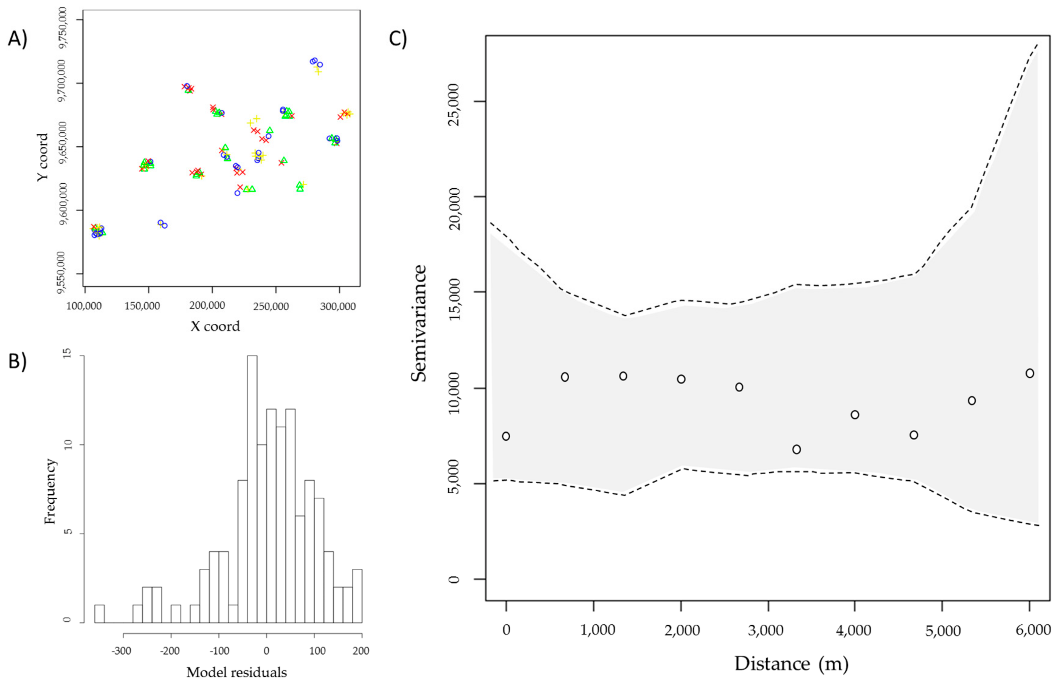
2.5. Geostatistical Analysis of Random Forest Model Residuals

Geostatistical analysis is used to explore the spatial autocorrelation of the model residuals and evaluate whether model residuals data are independent (in the case of absence of autocorrelation) [69]. The presence of spatial autocorrelation or spatial structure of the model residuals would refer to any patterns of gradients or cluster within the data that the AGB Random Forest model would not have adequately been able to capture. To explore this spatial structure, we estimated an omnidirectional variogram at short distances (6 km) on Random Forest residuals, and we used the usual permutation test to compute a bi-lateral confidence band of pure spatial randomness [70,71].

2.6. Comparison with Avitabile et al. [23] AGB Dataset

The available Avitabile et al. [23] forest pantropical biomass map that displays aboveground biomass density in units of Mg·ha−1 at a 920-m spatial resolution was used to compare the spatial distribution of aboveground biomass of the degraded forest with the Random Forest predicted map. In the Amazon basin, the Avitabile AGB map provides lower RMSE and bias compared to the Baccini and Saatchi pantropical maps [21,22,23]. However, at the regional scale (e.g., Paragominas municipality), the Avitabile map can present error patterns because the quality reference data of the highly degraded forest were lacking and could not be used to calibrate the model [23].

2.7. Comparison with Degraded Forest Typology

To conduct a field validation of the predicted aboveground biomass values, we built a degraded forest typology based on the observation of 140 forest sites in May 2015. Each observation is associated with a GPS point (Garmin 60CSx, Garmin, Olathe, KS, USA), a description of the forest site and illustrative photos. We extracted the values of the predicted AGB at the location of each forest site. We finally used one-way ANOVA with post hoc Tukey tests to evaluate differences in predicted AGB between the different forest classes of the typology.
This typology is a result of the combination of in-situ qualitative indicators of forest degradation and semi-quantitative observations of the forest structure. First, we noted the presence or absence of fire and logging marks (burned trees, strains, trunks, logging trails), of pioneer species (mainly Cecropia species), which may indicate a recent opening of the canopy, and of trees with a diameter at breast height (DBH) greater than 80 cm. Then, we measured canopy height and the number of vegetative strata using a laser rangefinder and estimated the forest canopy texture (roughness) and the percentage of gaps between emergent trees. These four forest structure indicators provide relevant information on the vertical and horizontal process of forest degradation.
In order to make the typology representative of the diversity of degraded forest types (conserved, legally logged, illegally logged and/or burned), we made sure that the sampling covered the different forest landscapes and main zoning that can be found in Paragominas (see Figure 1).

2.8. Computational Aspects

Except for the statistics performed with the software ArcGIS (Esri, Redlands, CA, USA), all developments were programmed under the R environment. We used the Raster, Random Forest, shapefile, rgdal, geoR and gstat packages [62,71,72,73,74,75].

3. Results

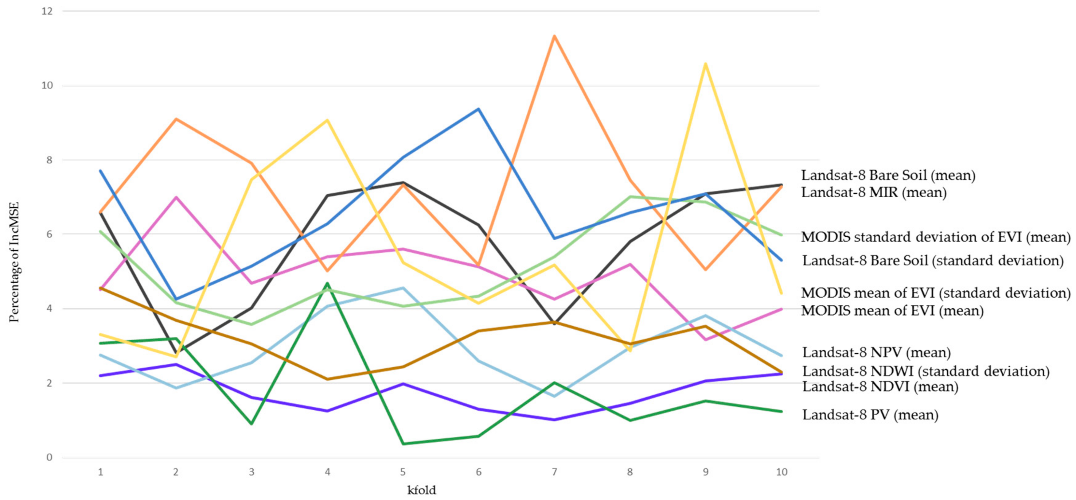
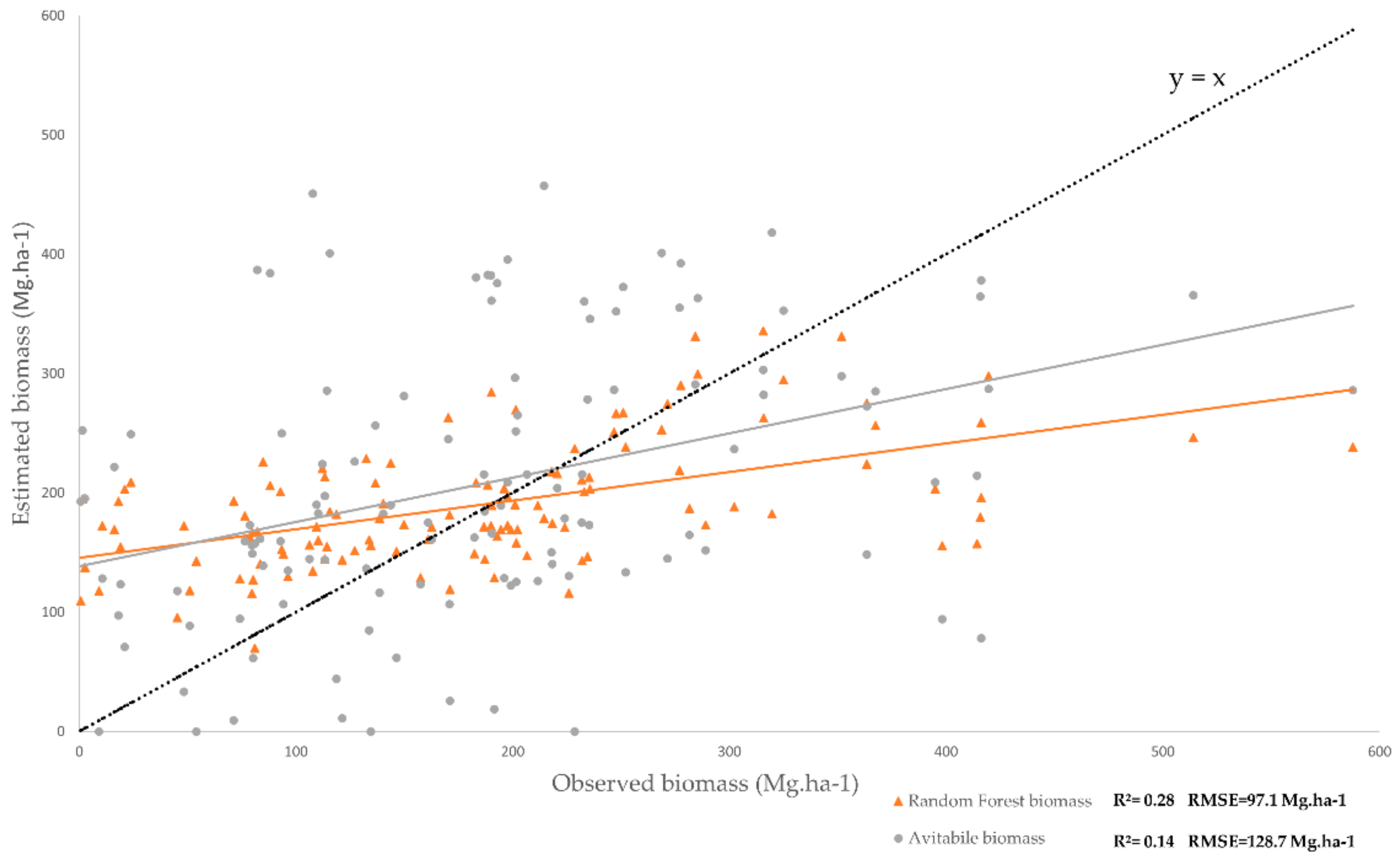
3.1. Model and Indicator Performance

The mean variance explained by the random forest model is 28%, with a root mean squared residual error (RMSE) of 97.1 Mg·ha−1. Depending on the AGB calibrated data and the associated remotely sensed indictors, the random forest model performs differently with an explained variance that ranges between 24% and 30% and an RMSE that ranges between 75.7 and 101.2 Mg·ha−1 (Table 2).
Six indicators (out of the 76) contribute the most to the 10 regression models, showing the highest and most stable IncMSE scores (Figure 3). Three are derived from MODIS: mean of annual standard deviation EVI, mean and standard deviation of annual mean EVI and three from Landsat: mean infra-red (MIR), mean and standard deviation of bare soils.

3.2. Geostatistical Analysis of Random Forest Model Residuals

The main spatial variability in the AGB data was captured by the Random Forest model, and no additive spatial variability can be explained through model residual interpolation. Figure 4 shows a flat empirical variogram contained within the confidence band which validates the absence of spatial structure within the Random Forest model residuals. We found similar results at smaller (0 to 1500 m) and larger (0–200,000 m) spatial scales. The distribution of the residuals shows an overall overestimation (high frequency of positive values, Figure 4B), which is important to consider when predicting AGB for the Paragominas municipality.

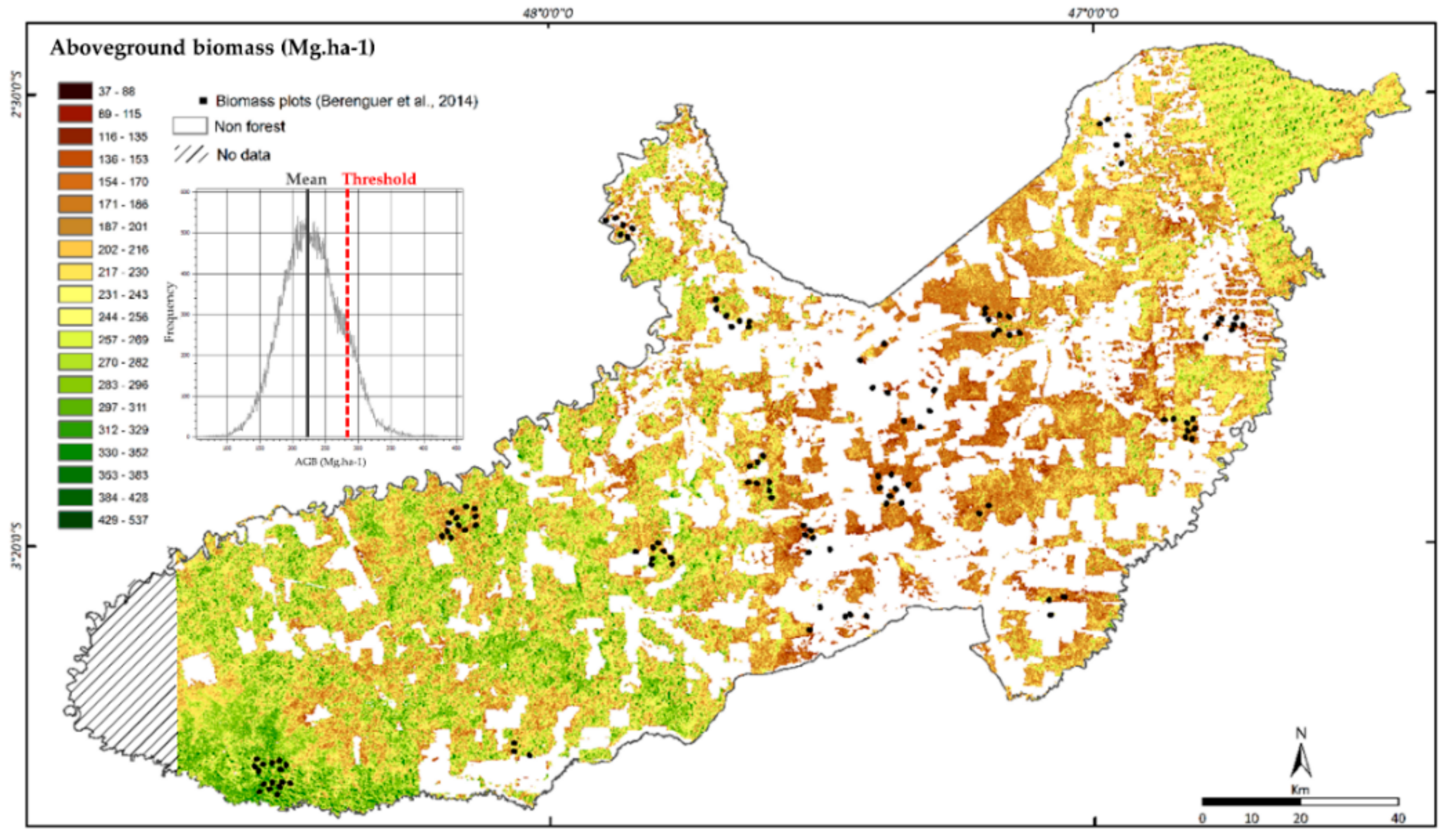
3.3. Above Ground Biomass Map

The range of AGB predicted values was large, spanning from 57 to 454 Mg·ha−1. AGB was unequally spatially distributed over the municipality (Figure 5). The forests in the 80-km-wide central corridor have the lowest AGB values and are highly fragmented. The forests in the far-eastern and western part of the municipality contain the highest AGB. The percentage of degraded forest (below the threshold of 286 Mg·ha−1, see Section 2.2) reached 87%.

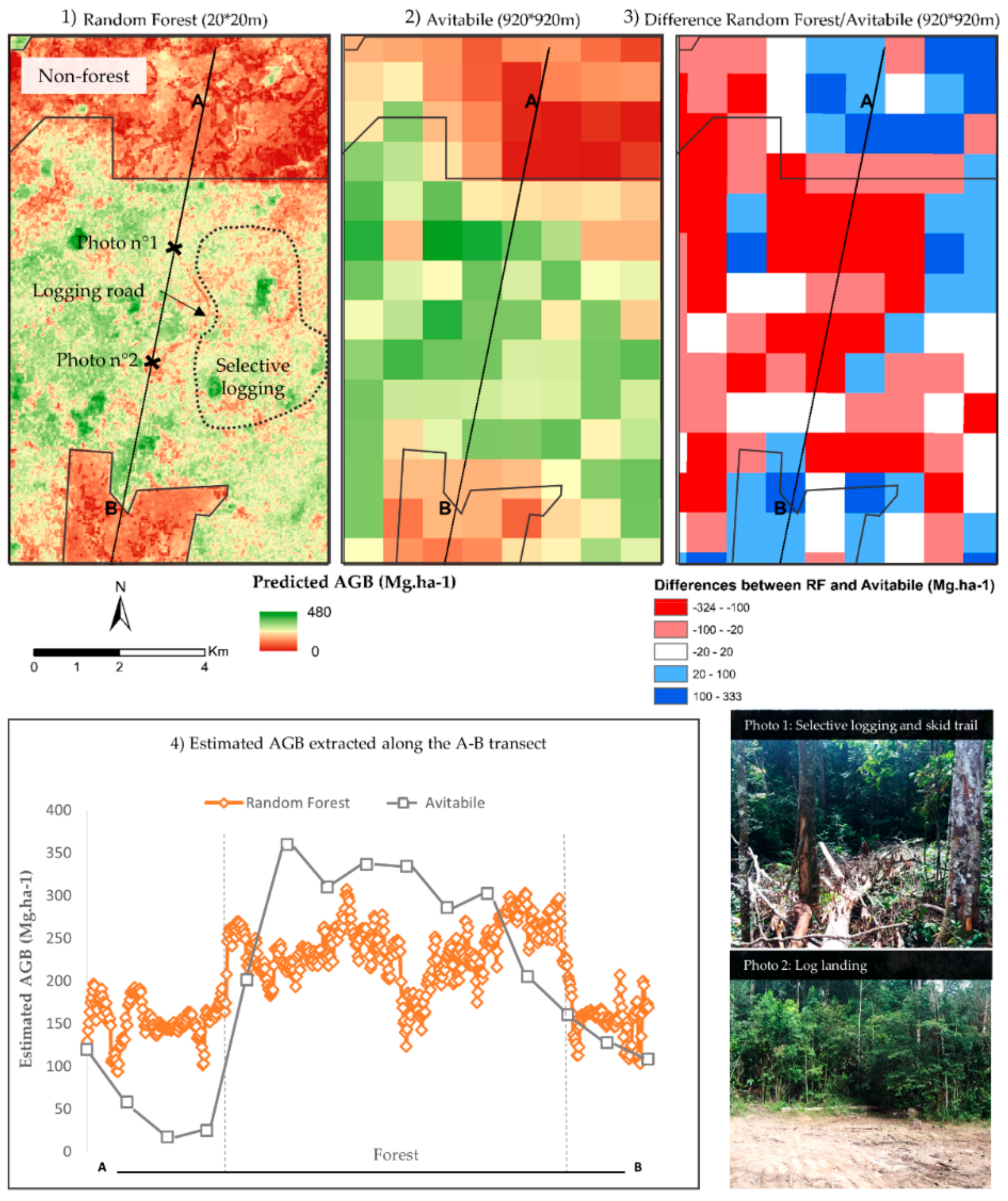
3.4. Comparison with Avitabile Pantropical Biomass Map

Figure 6 shows that our Random Forest model is more accurate than the Avitabile AGB map (R2 higher and RMSE lower). The two models tend to overestimate for values of AGB lower than 200 Mg·ha−1 and underestimate for values higher than 300 Mg·ha−1. Despite the fact that the Random Forest has a higher explained variance and lower RMSE, the Avitabile dataset has a better potential to capture the large variability of AGB, particularly for extreme values where the dispersion follows the identity line. Random forest data are overall less scattered than Avitabile but display a much lower deviation between estimated and observed AGB for values from 100 to 300 Mg·ha−1 (Random Forest R2 = 0.28, Avitabile R2 = 0.14). This result is particularly interesting in the case of degraded forests where biomass values are contained within this window (Table 1).
The Avitabile map is less detailed than the Random Forest biomass map. It can be explained by the difference of spatial resolution between the two datasets and also the contribution of local remotely sensed indicators. After aggregating the Random Forest biomass map at the resolution of Avitabile’s (Figure 7(3)), the difference between these two datasets shows similar AGB estimation in non-degraded areas and an overestimation of AGB values in degraded (logged) forests for Avitabile’s dataset (differences lower than −100 Mg·ha−1). The Random Forest map captures small-scale forest disturbances such as roads, i.e., skids trails and log-landing areas and canopy gaps (pictures 1 and 2). It also displays lower biomass values around the areas impacted by selective logging. These finely detailed forest disturbances are not translated into the 920-m resolution Avitabile map. In this figure, we can see that the forest-non forest transition is much better detailed with the Random Forest map than with Avitabile maps. The transect (Figure 7(4)) and the map show that the north forest edge is more degraded (probably burned with agriculture encroachment) than the south edge where the transition between the two land uses is much clearer and sharper (Transect A–B, see Figure 1 for its location). At this local scale, Avitabile data appear to stretch the values of AGB and thus smoothen the distribution of AGB in transition areas.

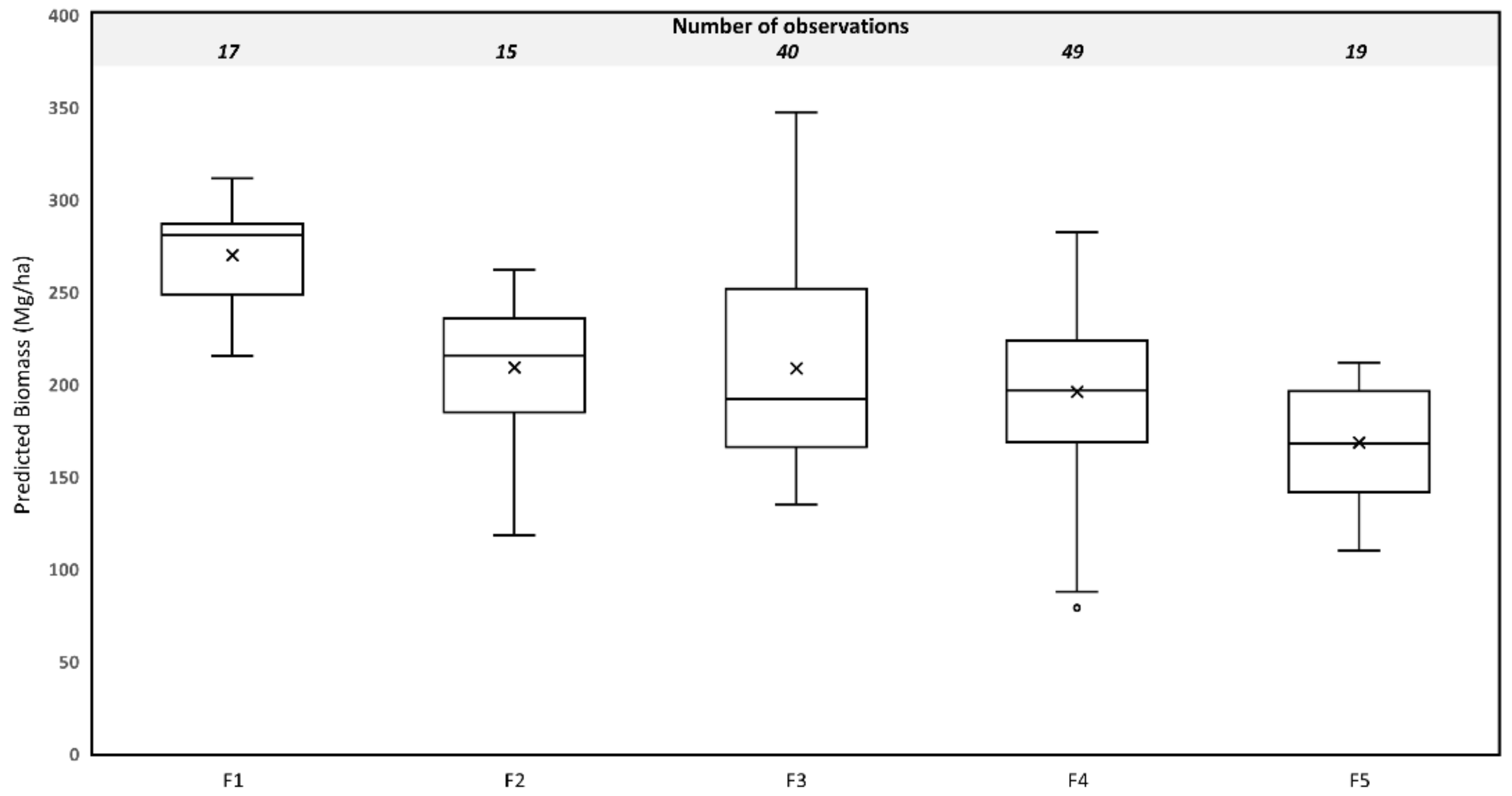
3.5. Comparison with Degraded Forest Typology

The less degraded forest type (type F1) presents a closed canopy above 35 m, no signs of human impact and 4 vegetative strata defined as follows: the shrub layer below 5 m, the under canopy layer located around 15 m, the canopy layer at 25 m and the emergent layer that goes beyond 35 m. The most valuable tree species harvested first are the emergent trees with a large diameter (higher than 80 cm). This selective logging can cause small degradation vertically, with an impacted and lower canopy and also horizontal damages generated by the extraction of the tree (type F2). When the selective logging becomes more intense (type F3), all the trees taller than 35 m and larger than 80 cm diameter are harvested, which causes a lowering of the canopy line at 25 m and big gaps inside the forest structure with the presence of skid tracks, broken and unrooted trees, log landing and other logging roads. Consequently, the degraded forest is much more sensitive to drought and fires, which can lead to severe disturbance, lowering the canopy at 15 m with only two remaining vegetative strata. This degraded forest type (F4) is often characterized by a high density of vegetative regrowth (pioneers species). Trees with DBH less than 80 cm are also harvested which causes an opened and destructed canopy. Finally, the intensification of fire leads to the most degraded type (F5) with only the shrub layer remaining and a few trees from the under canopy layer (Figure 8).
The typology of the degraded forest allows us to evaluate the relevance of the regional forest AGB mapping at the stand scale. The boxplots of Figure 9 show a relationship between the intensity of degradation identified in the field and the Random Forest prediction. We can assume the homogeneity of variances in the five degraded forest types (p-value = 0.09 > 0.05). Among the five types, only type F1 is significantly different from the other types F2, F3, F4, F5 (ANOVA test with p-value < 0.05). Degraded type F1 presented the highest values of AGB (average of 270 Mg·ha−1). Types F2, F3, F4, F5 had statistically similar values of AGB (200 Mg·ha−1), although we found a decreasing trend in the mean predicted AGB.

4. Discussion and Conclusions

In this paper, we propose a novel approach to model and map AGB of degraded forests at the regional scale, which provides more detailed and accurate information than the pantropical dataset. We demonstrated that the model captures all spatial variability of the AGB data and identified the most robust remotely sensed indicators. Besides the model bias in underestimating AGB values greater than 300 Mg·ha−1, this AGB map constitutes key spatial information for the future management of degraded forest.

4.1. Model Performance Analysis

  • Extraction and selection of suitable indicators from remote sensing and future promising development in AGB mapping
There is a need to rank and prioritize the most suitable indicators to characterize degraded forests from multisource remote sensing [33,34,76,77]. Our results show that Landsat spectral unmixing bare soil, mid infrared and MODIS EVI standard deviation from the 2001 to 2014 time series were the most suitable indicators to model AGB and are the less data input driven. These indicators thus have the highest potential to map AGB. Unmixing approaches did perform well in our case, which confirms reports of other authors [15,40] within the Amazon forest landscape. The bare soil Landsat indicator best translates the proportion of bare soil within a 30 × 30 m Landsat pixels while mid infrared is sensitive to humidity and therefore to forest structure and functioning [33]. These results are coherent with the degradation process happening in the Paragominas forest. The emergent and most valuable trees are targeted first through legal and illegal selective logging which triggers a vertical and horizontal opening of the canopy [78]. This type of degradation directly affects the internal forest structure, which leads to forest drying and a decrease in the local forest evapotranspiration and photosynthetic activity. Another degradation type is located along forest edges, which are always very degraded and impacted by local drying effect, fire or slow encroachment due to agriculture expansion (i.e., swidden agriculture) [79]. The MODIS compiled standard deviation of EVI represents the stability over time of the annual mean EVI and thus annual photosynthetic activity. A drop in this activity in one particular year will lead to a high standard deviation value and information on potential degradation activity [79].
The other indicators have a much lower performance score, which indicates a lower sensitivity to the AGB range of values. The usual vegetation indices extracted from Landsat such as NDVI or SAVI are not sensitive enough for AGB of degraded forests. This may be related to the over saturation of the signal in the case of a tropical forest canopy and the measured photosynthesis activity, which do not allow differentiation between two types of degraded forests [56].
For radar data, one single data and related derived indicators (intensity coefficients and texture) are not sensitive enough to model AGB. To further develop this modelling approach, radar needs to be used as time series data, which would provide better information on the forest canopy status. Further investigation is also required on the preprocessing steps (e.g., filtering noise method) and on the derived texture indicators. To the extent of our knowledge, degraded forest structure and status remain understudied, with a lot of technical aspects (frequency of the time series, spatial resolution, polarizations, incident angles and frequency bands) that need to be tackled [80,81,82].
The integration of Sentinel-1 and Sentinel-2 time series would be an interesting way to improve the model performance combined with daily Planet images that can map at 3-m resolution the forest canopy. Very high resolution remote sensing offers a unique opportunity to characterize degraded forest structure using canopy texture mapping [60,83]. These analysis provide perspective for future space-borne LIDAR and RADAR data satellites (US GEDI mission and ESA Biomass) which will enable us to provide data sets on forest structure dynamics and forest biomass around the pantropical belt [84].
  • Identification of proper algorithms to develop biomass estimation models and their related uncertainty analysis
Although the model is robust because it has been trained and tested 10 times on independent and randomly selected datasets, we identified three potential error sources. First, the limitations can be linked to the large diversity of degraded forest types that are modelled and the limited number of ground truth data. More in-situ AGB data would help to train the model on large portion of the data set and better capture its underlying trend [85]. Then, a certain time gap between the collection of AGB and the remote sensing data needs to be noted and accounted. This gap is due to remote sensing data quality and availability and can be up to 5 years in the case of Sentinel-1 images. In the case of MODIS time series, there is also a temporal gap as we modelled single date forest status (i.e., AGB) with temporal indicators that are sensitive to photosynthetic activity dynamics. These temporal mismatches could introduce some uncertainty in the model. However, in light of the minimal increases in AGB within burned and illegally logged forests (representing 88 out of 121 field plots) over a five-year period, we do not consider this uncertainty to be meaningful [86]. Finally, the resampling of the remote sensing indicators to a higher resolution (20 m resolution) may introduce bias referring to the “ecological fallacy” problems [87]. These problems are recurrent in the aggregation/disaggregation of remote sensing data and could be minimized by adapting the field collection protocol to the remote sensing data.
Despite these limitations and the low variance explained, we demonstrated that all spatial variability of the AGB data has been captured by the model through its input indicators. This gives interesting insights into how to improve local models to characterize degraded forests using biomass and how to quantify the influence of input indicators on the final modelling result.
  • Comparison with existing AGB maps
When comparing with pantropical datasets such as the Avitabile AGB map, we noted differences in the statistical accuracy with local AGB datasets and in the levels of details which are particularly important for degraded forest biomass mapping. Avitabile data do not capture all the details of local AGB distribution in small-scale degraded and complex mosaic forest due mainly to their coarse spatial resolution. Transition zones from forest/non-forest areas are better and more precisely described using local trained models, where logging roads, degraded forest edges and other distribution are mapped.

4.2. AGB Spatial Distribution in the Municipality

In the map produced, the spatial distribution of AGB varies depending on land-uses and landscape organization [88]. Degraded forests are dominant in the Paragominas forest landscape. The central corridor is a mosaic of agricultural lands (agribusiness) dominated by large-scale soybean cultivation and pasturelands and with fragmented patches of degraded forests. Forest biomass values range between 100 to 150 Mg·ha−1 with the lowest values within the first 200 m of forest edge which is consistent with previous studies [79]. Forest fragmentation is even more important in smallholder areas (see Figure 1) where population density is high. These areas were major charcoal production hotspots (prohibited since 2008), which caused severe impacts on the forest resource. The transition between these areas and the indigenous protected reserve is sharp within the forest AGB values (with AGB higher than 250 Mg·ha−1 in the reserve).

4.3. Characterization of Degraded Forests

From a field point of view, degraded forests are a gradient of forest types marked by a certain canopy height and forest structure that vary depending on the intensity of past degradation trajectories. The five-class typology does not represent all the complexity of degraded forests but remains relevant in terms of modelled forest biomass. Besides the fact that only type F1 was significantly different from the four others, we found an interesting trend in the modelled biomass that requires further investigation. Type F3 presented the highest variability, which could be linked with an over-evaluation of the level of degradation in the field and the disproportionate size sample of this class. Type 5, the most degraded stage, presents the lowest predicted biomass (around 150 Mg·ha). These findings accord with those identified by the RAS team during the collection of in-situ AGB data (Table 1). This typology based on the observation of structural parameters (canopy height, number of vegetative strata, canopy rugosity, presence of emergent trees) constitutes a first step in the characterization of degraded forests which could help in the calibration and validation of other forest biomass and carbon stock assessment or the monitoring of forest degradation [76,89]. It also summarizes a one-shot time visualization of the status of degraded forests. From this, the next priority is to monitor the dynamics of degraded forest status over time using time series remote sensing [90].

4.4. How Can These Data Be Useful for Forest Management at the Regional Scale?

Besides the limitations of the proposed modelling approach and the evaluated bias, we showed the importance of regional AGB mapping in Paragominas human-modified forest landscapes, in particular with the capacity to identify patterns of different forest status values linked with degradation and agricultural activities at the regional scale. This agricultural frontier is characterized by fragmented forest impacted by the accumulation of small-scale human disturbances that cannot be captured by pantropical databases, by forest field inventories or by high detailed/low extent coverage remote sensing sources (LIDAR).
In the context of zero deforestation commitment, this forest AGB modelling and mapping is particularly important in order to provide to decision makers with spatially detailed information on the status of the 50% remnant forest [91,92]. The agricultural expansion over forest areas is now severely restricted [50]. Hence, the sustainable management of degraded forests is becoming a priority in order to enhance forest resources at different levels of disturbance [93] as much as the urgent obligation to prevent further degradation. The quantification of the forest status and the understanding of the drivers of degradation are necessary in order to improve the management of forest landscape.

Author Contributions

Study conception and design: C.B., L.B., V.G., J.O., I.T., P.S., F.L., A.F.H. Acquisition of data: C.B., L.B., I.T., E.B., V.G., F.L., A.F.H. Data Analysis and model building: C.B., J.-S.B., G.C. Drafting of the manuscript: C.B. Critical revisions: C.B., L.B., J.O., V.G., E.B., J.-S.B.

Funding

This study is part of a PhD project funded by the Cirad and the CIAT. The authors are grateful to the ECOTERA project funded by the French National Agency for Research (ANR) (grant agreement ANR-13-AGRO-0003). The authors thank the Forest Tree and Agrofrestry program of CGIAR for their financial support for open access fees.

Acknowledgments

This is publication number 67 of the Sustainable Amazon Network series. The authors are grateful to the Rede Amazônia Sustentável (RAS) team for sharing the AGB data and the Platform in partnership Amazonia (https://www.dp-amazonie.org/en). The authors thank Joice Ferreira, Solen Le Clec’h and Nicolas Baghdadi for valuable discussions.

Conflicts of Interest

The authors declare no conflict of interest.

Appendix A

Table A1. Remote sensing metadata and derived indicators.
Satellite SourcesLinksDateResolutionIDPreprocessingSpectral BandsIndicators
MODIShttp://modis.gsfc.nasa.gov/2001–2014 every 16 days250 mMOD13Q1:h13v09Georeferenced, removed cloud covered pixels, atmospheric correctionsRed (620–670 nm), Near infrared (841–876 nm)EVI mean, EVI standard deviation, EVI variance
Landsat 8http://earthexplorer.usgs.gov/27 October 2014
16 September 2014
12 June 2014
30 mLC8220622014300LGN00
LC8220622014259LGN00
LC8220622014163LGN00
Georeferenced and reflectance productBlue (450–515 nm), Green (525–600 nm), Red (630–680 nm), Near Infrared (845–885 nm), Short Wave Infrared (1560–1660 nm)PV, NPV, Bare Soil (Claslite unmixing indicators)
B, G, R, NIR, SWIR
NDVI, RVI, RI, SAVI, NDWI, MSAVI, GEMI, WDVI, NDTI, TSAVI, NDPI, IPVI, TNDVI (Orfeo Toolbox derived indicators)
ALOS-1 PALSARhttp://global.jaxa.jp/26 May 2010
18 July 2010
23 July 2010
28 July 2010
7 August 2010
9 September 2010
25 mN00W050Georeferenced and calibrated:
(1) gamma [dB]
(2) sigma [dB]
L-band (1.27 GHz), dual-polarisation (HH, HV)Gamma [dB], Sigma [dB]
Sentinel-1https://scihub.esa.int/4 May 201510 mL1 (Ground Range Detected)Calibration and georeferenced (Sentinel-Toolbox Software)C-band dual-polarisation (VV, VH)Sigma [dB]
Grey Level Co-occurence matrix (9 × 9 pixels): Contrast, Dissimilarity, Energy, Entropy, Correlation, Mean, Variance, Homogeneity, Maximum (Sentinel Toolbox derived indicators)

References

  1. Houghton, R.A. The emissions of carbon from deforestation and degradation in the tropics: Past trends and future potential. Carbon Manag. 2013, 4, 539–546. [Google Scholar] [CrossRef]
  2. Simula, M.; Mansur, E. A global challenge needing local response. Unasylva 2011, 62, 238. [Google Scholar]
  3. Baccini, A.; Walker, W.; Carvalho, L.; Farina, M.; Sulla-Menashe, D.; Houghton, R.A. Tropical forests are a net carbon source based on aboveground measurements of gain and loss. Science 2017, 358, 230–234. [Google Scholar] [CrossRef] [PubMed]
  4. Barlow, J.; Lennox, G.D.; Ferreira, J.; Berenguer, E.; Lees, A.C.; Nally, R.M.; Thomson, J.R.; Ferraz, S.F.D.B.; Louzada, J.; Oliveira, V.H.F.; et al. Anthropogenic disturbance in tropical forests can double biodiversity loss from deforestation. Nature 2016, 535, 144–147. [Google Scholar] [CrossRef] [PubMed]
  5. Thompson, I.D.; Guariguata, M.R.; Okabe, K.; Bahamondez, C.; Nasi, R.; Heymell, V.; Sabogal, C. An operational framework for defining and monitoring forest degradation. Ecol. Soc. 2013, 18, 20. [Google Scholar] [CrossRef]
  6. Putz, F.E.; Redford, K.H. The importance of defining ‘forest’: Tropical forest degradation, deforestation, long-term phase shifts, and further transitions. Biotropica 2010, 42, 10–20. [Google Scholar] [CrossRef]
  7. Lamb, D.; Erskine, P.D.; Parrotta, J.A. Restoration of degraded tropical forest landscapes. Science 2005, 310, 1628–1632. [Google Scholar] [CrossRef] [PubMed]
  8. PRODES—Coordenação-Geral de Observação da Terra. Available online: http://www.obt.inpe.br/OBT/assuntos/programas/amazonia/prodes (accessed on 13 April 2018).
  9. Hansen, M.C.; Stehman, S.V.; Potapov, P.V. Quantification of global gross forest cover loss. Proc. Natl. Acad. Sci. USA 2010, 107, 8650–8655. [Google Scholar] [CrossRef] [PubMed]
  10. Fearnside, P.M. Deforestation in Brazilian Amazonia: History, rates, and consequences. Conserv. Biol. 2005, 19, 680–688. [Google Scholar] [CrossRef]
  11. Nepstad, D.; Soares-Filho, B.S.; Merry, F.; Lima, A.; Moutinho, P.; Carter, J.; Bowman, M.; Cattaneo, A.; Rodrigues, H.; Schwartzman, S.; et al. The end of deforestation in the Brazilian Amazon. Science 2009, 326, 1350–1351. [Google Scholar] [CrossRef] [PubMed]
  12. DEGRAD—Coordenação-Geral de Observação da Terra. Available online: http://www.obt.inpe.br/OBT/assuntos/programas/amazonia/degrad (accessed on 10 April 2018).
  13. Florestas Do Brasil em Resumo 2013. Available online: http://www.florestal.gov.br/publicacoes/572-florestas-do-brasil-em-resumo-2013 (accessed on 10 April 2018).
  14. Asner, G.P.; Knapp, D.E.; Broadbent, E.N.; Oliveira, P.J.; Keller, M.; Silva, J.N. Selective logging in the Brazilian Amazon. Science 2005, 310, 480–482. [Google Scholar] [CrossRef] [PubMed]
  15. Souza, C., Jr.; Siqueira, J.V.; Sales, M.H.; Fonseca, A.V.; Ribeiro, J.G.; Numata, I.; Cochrane, M.A.; Barber, C.P.; Roberts, D.A.; Barlow, J.; et al. Ten-Year landsat classification of deforestation and forest degradation in the Brazilian Amazon. Remote Sens. 2013, 5, 5493–5513. [Google Scholar] [CrossRef]
  16. Thompson, I.; Mackey, B.; McNulty, S.; Mosseler, A. Forest Resilience, Biodiversity, and Climate Change. A synthesis of the biodiversity/resilience/stability relationship in forest ecosystems. Secr. Conv. Biol. Divers. Montr. 2009, 43, 1–67. [Google Scholar]
  17. Potapov, P.; Hansen, M.C.; Laestadius, L.; Turubanova, S.; Yaroshenko, A.; Thies, C.; Smith, W.; Zhuravleva, I.; Komarova, A.; Minnemeyer, S.; et al. The last frontiers of wilderness: Tracking loss of intact forest landscapes from 2000 to 2013. Sci. Adv. 2017, 3, e1600821. [Google Scholar] [CrossRef] [PubMed]
  18. Bernier, P.Y.; Paré, D.; Stinson, G.; Bridge, S.R.J.; Kishchuk, B.E.; Lemprière, T.C.; Thiffault, E.; Titus, B.D.; Vasbinder, W. Moving beyond the concept of ‘primary forest’ as a metric of forest environment quality. Ecol. Appl. 2016, 27, 349–354. [Google Scholar] [CrossRef] [PubMed]
  19. Berenguer, E.; Ferreira, J.; Gardner, T.A.; Aragão, L.E.O.C.; De Camargo, P.B.; Cerri, C.E.; Durigan, M.; De Oliveira Junior, R.C.; Vieira, I.C.G.; Barlow, J. A large-scale field assessment of carbon stocks in human-modified tropical forests. Glob. Chang. Biol. 2014, 20, 3713–3726. [Google Scholar] [CrossRef] [PubMed] [Green Version]
  20. Bustamante, M.M.C.; Roitman, I.; Aide, T.M.; Alencar, A.; Anderson, L.O.; Aragão, L.; Asner, G.P.; Barlow, J.; Berenguer, E.; Chambers, J.; et al. Toward an integrated monitoring framework to assess the effects of tropical forest degradation and recovery on carbon stocks and biodiversity. Glob. Chang. Biol. 2016, 22, 92–109. [Google Scholar] [CrossRef] [PubMed]
  21. Saatchi, S.S.; Harris, N.L.; Brown, S.; Lefsky, M.; Mitchard, E.T.A.; Salas, W.; Zutta, B.R.; Buermann, W.; Lewis, S.L.; Hagen, S.; et al. Benchmark map of forest carbon stocks in tropical regions across three continents. Proc. Natl. Acad. Sci. USA 2011, 108, 9899–9904. [Google Scholar] [CrossRef] [PubMed]
  22. Baccini, A.; Goetz, S.J.; Walker, W.S.; Laporte, N.T.; Sun, M.; Sulla-Menashe, D.; Hackler, J.; Beck, P.S.A.; Dubayah, R.; Friedl, M.A.; et al. Estimated carbon dioxide emissions from tropical deforestation improved by carbon-density maps. Nat. Clim. Chang. 2012, 2, 182–185. [Google Scholar] [CrossRef]
  23. Avitabile, V.; Herold, M.; Heuvelink, G.B.M.; Lewis, S.L.; Phillips, O.L.; Asner, G.P.; Armston, J.; Ashton, P.S.; Banin, L.; Bayol, N.; et al. An integrated pan-tropical biomass map using multiple reference datasets. Glob. Chang. Biol. 2016, 22, 1406–1420. [Google Scholar] [CrossRef] [PubMed] [Green Version]
  24. Malhi, Y.; Wood, D.; Baker, T.R.; Wright, J.; Phillips, O.L.; Cochrane, T.; Meir, P.; Chave, J.; Almeida, S.; Arroyo, L.; et al. The regional variation of aboveground live biomass in old-growth Amazonian forests. Glob. Chang. Biol. 2006, 12, 1107–1138. [Google Scholar] [CrossRef]
  25. Asner, G.P.; Joseph Mascaro, J.; Muller-Landau, H.C.; Vieilledent, G.; Vaudry, R.; Rasamoelina, M.; Hall, J.S.; van Breugel, M. A universal airborne LiDAR approach for tropical forest carbon mapping. Oecologia 2012, 168, 1147–1160. [Google Scholar] [CrossRef] [PubMed]
  26. Asner, G.P. Tropical forest carbon assessment: Integrating satellite and airborne mapping approaches. Environ. Res. Lett. 2009, 4, 034009. [Google Scholar] [CrossRef]
  27. Asner, G.P.; Mascaro, J. Mapping tropical forest carbon: Calibrating plot estimates to a simple LiDAR metric. Remote Sens. Environ. 2014, 140, 614–624. [Google Scholar] [CrossRef]
  28. Fayad, M.; Baghdadi, N.; Fayad, I.; Vieilledent, G.; Bailly, J.-S.; Minh, D. Interest of integrating spaceborne LiDAR data to improve the estimation of biomass in high biomass forested areas. Remote Sens. 2017, 9, 213. [Google Scholar] [CrossRef]
  29. Mascaro, J.; Detto, M.; Asner, G.P.; Muller-Landau, H.C. Evaluating uncertainty in mapping forest carbon with airborne LiDAR. Remote Sens. Environ. 2011, 115, 3770–3774. [Google Scholar] [CrossRef]
  30. Longo, M.; Keller, M.; dos-Santos, M.N.; Leitold, V.; Pinagé, E.R.; Baccini, A.; Saatchi, S.; Nogueira, E.M.; Batistella, M.; Morton, D.C. Aboveground biomass variability across intact and degraded forests in the Brazilian Amazon. Glob. Biogeochem. Cycles 2016, 30, 1639–1660. [Google Scholar] [CrossRef]
  31. Baccini, A.; Laporte, N.; Goetz, S.J.; Sun, M.; Dong, H. A first map of tropical Africa’s above-ground biomass derived from satellite imagery. Environ. Res. Lett. 2008, 3, 045011. [Google Scholar] [CrossRef]
  32. Fayad, I.; Baghdadi, N.; Bailly, J.-S.; Barbier, N.; Gond, V.; Hajj, M.E.; Fabre, F.; Bourgine, B. Canopy height estimation in French Guiana with LiDAR ICESat/GLAS data using principal component analysis and random forest regressions. Remote Sens. 2014, 6, 11883–11914. [Google Scholar] [CrossRef] [Green Version]
  33. Hirschmugl, M.; Gallaun, H.; Dees, M.; Datta, P.; Deutscher, J.; Koutsias, N.; Schardt, M. Methods for mapping forest disturbance and degradation from optical earth observation data: A review. Curr. For. Rep. 2017, 3, 32–45. [Google Scholar] [CrossRef]
  34. Herold, M.; Román-Cuesta, R.M.; Mollicone, D.; Hirata, Y.; Van Laake, P.; Asner, G.P.; Souza, C.; Skutsch, M.; Avitabile, V.; Macdicken, K.; et al. Options for monitoring and estimating historical carbon emissions from forest degradation in the context of REDD+. Carbon Balance Manag. 2011, 6, 13. [Google Scholar] [CrossRef] [PubMed]
  35. Rappaport, D.; Morton, D.C.; Longo, M.; Keller, M.; Dubayah, R.; dos-Santos, M.N. Quantifying long-term changes in carbon stocks and forest structure from Amazon forest degradation. Environ. Res. Lett. 2018. [Google Scholar] [CrossRef]
  36. Achard, F.; Boschetti, L.; Brown, S.; Brady, M.; DeFries, R.; Grassi, G.; Herold, M.; Mollicone, D.; Mora, B.; Pandey, D.; et al. A Sourcebook of Methods and Procedures for Monitoring and Reporting Anthropogenic Greenhouse Gas Emissions and Removals Associated with Deforestation, Gains and Losses of Carbon Stocks in Forests Remaining Forests, and Forestation; GOFC-GOLD: Wageningen, The Netherlands, 2014. [Google Scholar]
  37. Lambin, E.F. Monitoring forest degradation in tropical regions by remote sensing: some methodological issues. Glob. Ecol. Biogeogr. 1999, 8, 191–198. [Google Scholar] [CrossRef]
  38. Gond, V.; Fayolle, A.; Pennec, A.; Cornu, G.; Mayaux, P.; Camberlin, P.; Doumenge, C.; Fauvet, N.; Gourlet-Fleury, S. Vegetation structure and greenness in Central Africa from Modis multi-temporal data. Philos. Trans. R. Soc. B Biol. Sci. 2013, 368, 20120309. [Google Scholar] [CrossRef] [PubMed] [Green Version]
  39. Asner, G.P.; Knapp, D.E.; Balaji, A.; Páez-Acosta, G. Automated mapping of tropical deforestation and forest degradation: CLASlite. J. Appl. Remote Sens. 2009, 3, 033543. [Google Scholar] [CrossRef]
  40. Tritsch, I.; Sist, P.; Narvaes, I.D.S.; Mazzei, L.; Blanc, L.; Bourgoin, C.; Cornu, G.; Gond, V. Multiple patterns of forest disturbance and logging shape forest landscapes in Paragominas. Braz. For. 2016, 7, 315. [Google Scholar] [CrossRef]
  41. Joshi, N.; Mitchard, E.T.; Woo, N.; Torres, J.; Moll-Rocek, J.; Ehammer, A.; Collins, M.; Jepsen, M.R.; Fensholt, R. Mapping dynamics of deforestation and forest degradation in tropical forests using radar satellite data. Environ. Res. Lett. 2015, 10, 034014. [Google Scholar] [CrossRef]
  42. Kuplich, T.M.; Curran, P.J.; Atkinson, P.M. Relating SAR image texture to the biomass of regenerating tropical forests. Int. J. Remote Sens. 2005, 26, 4829–4854. [Google Scholar] [CrossRef]
  43. Luckman, A.J.; Frery, A.C.; Yanasse, C.C.F.; Groom, G.B. Texture in airborne SAR imagery of tropical forest and its relationship to forest regeneration stage. Int. J. Remote Sens. 1997, 18, 1333–1349. [Google Scholar] [CrossRef]
  44. Haralick, R.M.; Shanmugam, K.; Dinstein, I. Textural features for image classification. IEEE Trans. Syst. Man Cybern. 1973, 6, 610–621. [Google Scholar] [CrossRef]
  45. Morel, A.C.; Saatchi, S.S.; Malhi, Y.; Berry, N.J.; Banin, L.; Burslem, D.; Nilus, R.; Ong, R.C. Estimating aboveground biomass in forest and oil palm plantation in Sabah, Malaysian Borneo using ALOS PALSAR data. For. Ecol. Manag. 2011, 262, 1786–1798. [Google Scholar] [CrossRef]
  46. Mitchard, E.T.A.; Saatchi, S.S.; Lewis, S.L.; Feldpausch, T.R.; Woodhouse, I.H.; Sonké, B.; Rowland, C.; Meir, P. Measuring biomass changes due to woody encroachment and deforestation/degradation in a forest–savanna boundary region of central Africa using multi-temporal L-band radar backscatter. Remote Sens. Environ. 2011, 115, 2861–2873. [Google Scholar] [CrossRef]
  47. Englhart, S.; Keuck, V.; Siegert, F. Aboveground biomass retrieval in tropical forests—the potential of combined X- and L-band SAR data use. Remote Sens. Environ. 2011, 115, 1260–1271. [Google Scholar] [CrossRef]
  48. Imazon—Instituto Do Homem e Meio Ambiente da Amazônia. Available online: http://imazon.org.br/en/ (accessed on 18 May 2018).
  49. IBGE, Paragominas. Available online: https://cidades.ibge.gov.br/brasil/pa/paragominas/panorama (accessed on 17 May 2018).
  50. Piketty, M.-G.; Poccard-Chapuis, R.; Drigo, I.; Coudel, E.; Plassin, S.; Laurent, F.; Marcello, T. Multi-level governance of land use changes in the Brazilian Amazon: Lessons from Paragominas, State of Pará. Forests 2015, 6, 1516–1536. [Google Scholar] [CrossRef] [Green Version]
  51. Viana, C.; Coudel, E.; Barlow, J.; Ferreira, J.; Gardner, T.; Parry, L. How does hybrid governance emerge? Role of the elite in building a Green Municipality in the Eastern Brazilian Amazon: Role of the elite in building a green municipality. Environ. Policy Gov. 2016, 26, 337–350. [Google Scholar] [CrossRef]
  52. Gardner, T.A.; Burgess, N.D.; Aguilar-Amuchastegui, N.; Barlow, J.; Berenguer, E.; Clements, T.; Danielsen, F.; Ferreira, J.; Foden, W.; Kapos, V.; et al. A framework for integrating biodiversity concerns into national REDD+ programmes. Biol. Conserv. 2012, 154, 61–71. [Google Scholar] [CrossRef]
  53. Gardner, T.A.; Ferreira, J.; Barlow, J.; Lees, A.C.; Parry, L.; Vieira, I.C.G.; Berenguer, E.; Abramovay, R.; Aleixo, A.; Andretti, C.; et al. A social and ecological assessment of tropical land uses at multiple scales: The Sustainable Amazon Network. Philos. Trans. R. Soc. B Biol. Sci. 2013, 368, 20120166. [Google Scholar] [CrossRef] [PubMed] [Green Version]
  54. Chave, J.; Andalo, C.; Brown, S.; Cairns, M.A.; Chambers, J.Q.; Eamus, D.; Fölster, H.; Fromard, F.; Higuchi, N.; Kira, T.; et al. Tree allometry and improved estimation of carbon stocks and balance in tropical forests. Oecologia 2005, 145, 87–99. [Google Scholar] [CrossRef] [PubMed]
  55. Mazzei, L.; Sist, P.; Ruschel, A.; Putz, F.E.; Marco, P.; Pena, W.; Ferreira, J.E.R. Above-ground biomass dynamics after reduced-impact logging in the Eastern Amazon. For. Ecol. Manag. 2010, 259, 367–373. [Google Scholar] [CrossRef]
  56. Huete, A.; Didan, K.; Miura, T.; Rodriguez, E.P.; Gao, X.; Ferreira, L.G. Overview of the radiometric and biophysical performance of the MODIS vegetation indices. Remote Sens. Environ. 2002, 83, 195–213. [Google Scholar] [CrossRef]
  57. Orfeo ToolBox—Orfeo ToolBox Is Not a Black Box. Available online: https://www.orfeo-toolbox.org/ (accessed on 13 April 2018).
  58. Mermoz, S.; le Toan, T.; Villard, L.; Réjou-Méchain, M.; Seifert-Granzin, J. Biomass assessment in the Cameroon savanna using ALOS PALSAR data. Remote Sens. Environ. 2014, 155, 109–119. [Google Scholar] [CrossRef]
  59. Shimada, M.; Itoh, T.; Motooka, T.; Watanabe, M.; Shiraishi, T.; Thapa, R.; Lucas, R. New global forest/non-forest maps from ALOS PALSAR data (2007–2010). Remote Sens. Environ. 2014, 155, 13–31. [Google Scholar] [CrossRef]
  60. Ploton, P.; Barbier, N.; Couteron, P.; Antin, C.M.; Ayyappan, N.; Balachandran, N.; Barathan, N.; Bastin, J.F.; Chuyong, G.; Dauby, G.; et al. Toward a general tropical forest biomass prediction model from very high resolution optical satellite images. Remote Sens. Environ. 2017, 200, 140–153. [Google Scholar] [CrossRef]
  61. Champion, I.; Germain, C.; da Costa, J.P.; Alborini, A.; Dubois-Fernandez, P. Retrieval of forest stand age from SAR image texture for varying distance and orientation values of the gray level co-occurrence matrix. IEEE Geosci. Remote Sens. Lett. 2014, 11, 5–9. [Google Scholar] [CrossRef]
  62. Breiman, L. Random forests. Mach. Learn. 2001, 45, 5–32. [Google Scholar] [CrossRef]
  63. Kohavi, R. A study of cross-validation and bootstrap for accuracy estimation and model selection. IJCAI 1995, 14, 1137–1145. [Google Scholar]
  64. Strobl, C.; Malley, J.; Tutz, G. An introduction to recursive partitioning: Rationale, application, and characteristics of classification and regression trees, bagging, and random forests. Psychol. Methods 2009, 14, 323–348. [Google Scholar] [CrossRef] [PubMed] [Green Version]
  65. Mascaro, J.; Asner, G.P.; Knapp, D.E.; Kennedy-Bowdoin, T.; Martin, R.E.; Anderson, C.; Higgins, M.; Chadwick, K.D. A tale of two ‘Forests’: Random forest machine learning aids tropical forest carbon mapping. PLoS ONE 2014, 9, e85993. [Google Scholar] [CrossRef] [PubMed]
  66. Goetz, S.J.; Baccini, A.; Laporte, N.T.; Johns, T.; Walker, W.; Kellndorfer, J.; Houghton, R.A.; Sun, M. Mapping and monitoring carbon stocks with satellite observations: A comparison of methods. Carbon Balance Manag. 2009, 4, 2. [Google Scholar] [CrossRef] [PubMed]
  67. Mutanga, O.; Adam, E.; Cho, M.A. High density biomass estimation for wetland vegetation using WorldView-2 imagery and random forest regression algorithm. Int. J. Appl. Earth Obs. Geoinf. 2012, 18, 399–406. [Google Scholar] [CrossRef]
  68. Borra, S.; di Ciaccio, A. Measuring the prediction error. A comparison of cross-validation, bootstrap and covariance penalty methods. Comput. Stat. Data Anal. 2010, 54, 2976–2989. [Google Scholar] [CrossRef]
  69. Rossi, R.E.; Mulla, D.J.; Journel, A.G.; Franz, E.H. Geostatistical tools for modeling and interpreting ecological spatial dependence. Ecol. Monogr. 1992, 62, 277–314. [Google Scholar] [CrossRef]
  70. Gräler, B.; Pebesma, E.; Heuvelink, G. Spatio-temporal interpolation using GSTAT. RFID J. 2016, 8, 204–218. [Google Scholar]
  71. Ribeiro, J.; Diggle, P.J. geoR: A package for geostatistical analysis. R News 2001, 1, 14–18. Available online: http://www.leg.ufpr.br/geoR/ (accessed on 25 May 2018).
  72. CRAN—Package Gstat. Available online: https://cran.r-project.org/web/packages/gstat/index.html (accessed on 13 April 2018).
  73. CRAN—Package Raster. Available online: https://cran.r-project.org/web/packages/raster/index.html (accessed on 13 April 2018).
  74. Stabler, B. CRAN—Package Shapefiles. Available online: https://cran.r-project.org/web/packages/shapefiles/ (accessed on 23 May 2018).
  75. Bivand, R.; Keitt, T.; Rowlingson, B.; Pebesma, E.; Sumner, M.; Hijmans, R.; Rouault, E.; Ooms, J. CRAN—Package Rgdal. Available online: https://cran.r-project.org/web/packages/rgdal/ (accessed on 23 May 2018).
  76. Mitchell, A.L.; Rosenqvist, A.; Mora, B. Current remote sensing approaches to monitoring forest degradation in support of countries measurement, reporting and verification (MRV) systems for REDD+. Carbon Balance Manag. 2017, 12, 9. [Google Scholar] [CrossRef] [PubMed]
  77. De Sy, V.; Herold, M.; Achard, F.; Asner, G.P.; Held, A.; Kellndorfer, J.; Verbesselt, J. Synergies of multiple remote sensing data sources for REDD+ monitoring. Curr. Opin. Environ. Sustain. 2012, 4, 696–706. [Google Scholar] [CrossRef]
  78. Ferreira, J.; Blanc, L.; Kanashiro, M.; Lees, A.C.; Bourgoin, C.; Freitas, J.V.D.; Gama, M.B.; Laurent, F.; Martins, M.B.; Moura, N.; et al. Degradação Florestal na Amazônia: Como Ultrapassar os Limites Conceituais, Científicos e Técnicos Para mUdar Esse Cenário; Embrapa Amazônia Oriental: Belém, Brazil, 2015. [Google Scholar]
  79. Briant, G.; Gond, V.; Laurance, S.G.W. Habitat fragmentation and the desiccation of forest canopies: A case study from Eastern Amazonia. Biol. Conserv. 2010, 143, 2763–2769. [Google Scholar] [CrossRef]
  80. Trisasongko, B.H. The use of polarimetric SAR data for forest disturbance monitoring. Sens. Imaging Int. J. 2010, 11, 1–13. [Google Scholar] [CrossRef]
  81. Deutscher, J.; Perko, R.; Gutjahr, K.; Hirschmugl, M.; Schardt, M. Mapping tropical rainforest canopy disturbances in 3D by COSMO-SkyMed Spotlight InSAR-Stereo data to detect areas of forest degradation. Remote Sens. 2013, 5, 648–663. [Google Scholar] [CrossRef]
  82. Solberg, S.; Astrup, R.; Breidenbach, J.; Nilsen, B.; Weydahl, D. Monitoring spruce volume and biomass with InSAR data from TanDEM-X. Remote Sens. Environ. 2013, 139, 60–67. [Google Scholar] [CrossRef]
  83. Barbier, N.; Couteron, P.; Proisy, C.; Malhi, Y.; Gastellu-Etchegorry, J.-P. The variation of apparent crown size and canopy heterogeneity across lowland Amazonian forests: Amazon forest canopy properties. Glob. Ecol. Biogeogr. 2010, 19, 72–84. [Google Scholar] [CrossRef]
  84. Le Toan, T.; Quegan, S.; Davidson, M.W.J.; Balzter, H.; Paillou, P.; Papathanassiou, K.; Plummer, S.; Papathanassiou, K.; Rocca, F.; Saatchi, S.; et al. The BIOMASS mission: Mapping global forest biomass to better understand the terrestrial carbon cycle. Remote Sens. Environ. 2011, 115, 2850–2860. [Google Scholar] [CrossRef]
  85. Guitet, S.; Hérault, B.; Molto, Q.; Brunaux, O.; Couteron, P. Spatial structure of above-ground biomass limits accuracy of carbon mapping in rainforest but large scale forest inventories can help to overcome. PLoS ONE 2015, 10, e0138456. [Google Scholar] [CrossRef] [PubMed] [Green Version]
  86. Blanc, L.; Echard, M.; Herault, B.; Bonal, D.; Marcon, E.; Chave, J.; Baraloto, C. Dynamics of aboveground carbon stocks in a selectively logged tropical forest. Ecol. Appl. 2009, 19, 1397–1404. [Google Scholar] [CrossRef] [PubMed]
  87. Robinson, W. Ecological correlations and the behavior of individuals. Int. J. Epidemiol. 2009, 38, 337–341. [Google Scholar] [CrossRef] [PubMed]
  88. Laurent, F.; Arvor, D.; Daugeard, M.; Osis, R.; Tritsch, I.; Coudel, E.; Piketty, M.-G.; Piraux, M.; Viana, C.; Dubreuil, V.; et al. Le tournant environnemental en Amazonie: Ampleur et limites du découplage entre production et déforestation. EchoGéo 2017, 41, 36–57. [Google Scholar] [CrossRef]
  89. DeVries, B.; Verbesselt, J.; Kooistra, L.; Herold, M. Robust monitoring of small-scale forest disturbances in a tropical montane forest using Landsat time series. Remote Sens. Environ. 2015, 161, 107–121. [Google Scholar] [CrossRef]
  90. DeVries, B.; Decuyper, M.; Verbesselt, J.; Zeileis, A.; Herold, M.; Joseph, S. Tracking disturbance-regrowth dynamics in tropical forests using structural change detection and Landsat time series. Remote Sens. Environ. 2015. [Google Scholar] [CrossRef]
  91. Climate-KIC|The EU’s Main Climate Innovation Initiative. Available online: http://www.climate-kic.org/ (accessed on 18 May 2018).
  92. Observatory of the Dynamics of Interactions between Societies and Environnement in the Amazon, ODYSSEA. Available online: https://odyssea-amazonia.org/ (accessed on 18 May 2018).
  93. Goldstein, J.E. The afterlives of degraded tropical forests: New value for conservation and development. In Environment and Society: Advances in Research; West, P., Brockington, D., Eds.; Berghahn Books: New York, NY, USA, 2014; Volume 5, pp. 124–140. [Google Scholar]
Figure 1. Map of Paragominas municipality in the northeastern part of the State of Para with the location of the biomass-collected plots, the degraded forest typology and the main zoning areas (extracted from [9]).
Forests 09 00303 g001
Figure 2. Workflow of the evaluation of the indicators performance in AGB modelling and mapping.
Forests 09 00303 g002
Figure 3. Explained indicator performance (Percentage of IncMSE) of the Random Forest model.
Forests 09 00303 g003
Figure 4. (A) Spatial distribution of the model residuals (blue, green, yellow and red colors for the respective four quartiles); (B) Histogram of the model residuals; (C) Variogram of biomass model residuals (The grey shape shows the confidence band interval expected for each distance class).
Forests 09 00303 g004
Figure 5. Random Forest predicted values of Aboveground Biomass across Paragominas municipality. In the western part of the municipality (stripped area), Sentinel-1 data was not available.
Forests 09 00303 g005
Figure 6. Observed (see Section 2.2) and estimated biomass from Avitabile [23] and the Random Forest model.
Forests 09 00303 g006
Figure 7. Comparison of AGB estimations, Random Forest, Avitabile [23] and the difference map (1–3 respectively) in a selected zone representing the transition between non-forest to forest area (see Figure 1 for precise location in Paragominas). The selective logging area and the logging road were validated during the field trip.
Forests 09 00303 g007
Figure 8. Five classes of degraded forest typology based on the observation of 140 forest sites in May 2015.
Forests 09 00303 g008
Figure 9. Boxplots of predicted values of AGB calculated for the five-class typology of degraded forest with the range (1st and 3rd quartile), the mean (line) and the median (cross).
Forests 09 00303 g009
Table 1. AGB collection data in the municipality of Paragominas (see [19]).
Forest TypeMean AGB (Mg·ha−1)Standard Deviation (Mg·ha−1)No. of Plots
Undisturbed primary forest371.896.913
Logged primary forest229.579.244
Logged and burnt primary forest145.873.444
Young secondary forest1.10.52
Intermediate secondary forest57.638.312
Old secondary forest92.258.45
Abandoned plantation54.1/1
Table 2. Random Forest model performance (mean squared residuals and percentage of variance explained for each of the 10 k-fold random forest models).
Random Forest k-fold 112345678910Average
Mean of squared residuals (Mg·ha−1)97.895.5100.591.899.6100.393.975.797.8101.297.1
Percentage of variance explained2624253026222730262528
1 Number of Trees: 500, No. of Indicators Tried at Each Split: 25.

