LR Parsing for LCFRS

Abstract

LR parsing is a popular parsing strategy for variants of Context-Free Grammar (CFG). It has also been used for mildly context-sensitive formalisms, such as Tree-Adjoining Grammar. In this paper, we present the first LR-style parsing algorithm for Linear Context-Free Rewriting Systems (LCFRS), a mildly context-sensitive extension of CFG which has received considerable attention in the last years in the context of natural language processing.

1. Introduction

In computational linguistics, the modeling of discontinuous structures in natural language, i.e., of structures that span two or more non-adjacent portions of the input string, is an important issue. In recent years, Linear Context-Free Rewriting System (LCFRS) [1] has emerged as a formalism which is useful for this task. LCFRS is a mildly context-sensitive [2] extension of CFG in which a single non-terminal can cover $k\in \mathbb{N}$ continuous blocks of terminals. CFG is a special case of LCFRS where $k=1$. 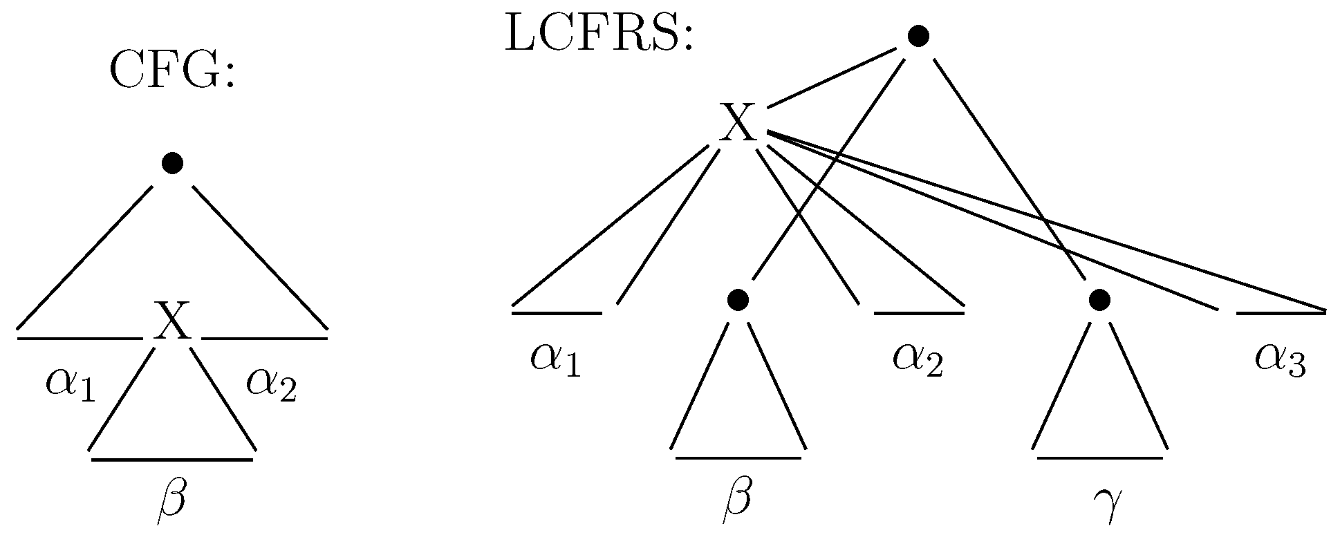In CFG, only embedded structures can be modelled. In LCFRS, in contrast, yields can be intertwined. The schematically depicted derivation trees in Figure 1 illustrate the different domains of locality of CFG and LCFRS. As can be seen, in the schematic CFG derivation, X contributes a continuous component β to the full yield. In the schematic LCFRS derivation, however, X contributes three non-adjacent components to the full yield. Intuitively speaking, the difference between LCFRS and CFG productions is that the former allow for arguments on their non-terminals. Each argument spans a continuous part of the input string, i.e., an argument boundary denotes a discontinuity in the yield of the non-terminal. The production itself specifies how the lefthand side non-terminal yield is built from the yields of the righthand side non-terminals. In the example, the X node in the schematic LCFRS tree would be derived from a production which, on its left hand side, has a terminal $X(x_1,x_2,x_3)$. Note that CFG non-terminals can consequently be seen as LCFRS non-terminals with an implicit single argument.

LCFRS has been employed in various subareas of computational linguistics. Among others, it has been used for syntactic modeling. In syntax, discontinuous structures arise when a displacement occurs within the sentence, such as, e.g., with topicalization. Constructions causing discontinuities are frequent: In the German TiGer treebank [3], about a fourth of all sentences contains at least one instance of discontinuity [4]; in the English Penn Treebank (PTB) [5], this holds for about a fifth of all sentences [6]. Below, three examples for discontinuities are shown. In (1), the discontinuity is due to the fact that a part of the VP is moved to the front. In (2), the discontinuity comes from the topicalization of the pronoun Darüber. (3), finally, is an example for a discontinuity which has several parts. It is due to a topicalization of the prepositional phrase Ohne internationalen Schaden, and scrambling [7] of elements after the verb.

(1)

Selbst besucht hat er ihn nie

Personally visited has he him never

“He has never visited him personally”

(2)

Darüber muss nachgedacht werden

About it must thought be

“One must think about that”

(3)

Ohne internationalen Schaden könne sich Bonn von dem Denkmal nicht distanzieren

Without international damage could itself Bonn from the monument not distance

“Bonn could not distance itself from the monument without international damage.”

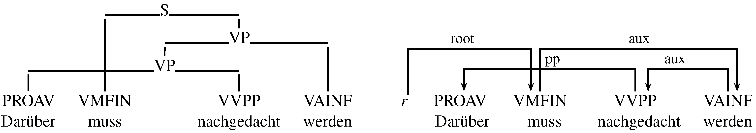
The syntactic annotation in treebanks must account for discontinuity. In a constituency framework, this can be done by allowing crossing branches and grouping all parts of a discontinuous constituent under a single node. Similarly in dependency syntax [8], words must be connected such that edges end up crossing. As an example, Figure 2 shows both the constituency and dependency annotations of (2). While the discontinuous yields inhibit an interpretation of either structure as a CFG derivation tree, both can immediately been modeled as the derivation of an LCFRS [4,9].

In grammar engineering, LCFRS and related formalisms have been employed in two ways. Grammatical Framework (GF) is actively used for multilingual grammar development and allows for an easy treatment of discontinuities, see [11] for details. GF is an extension of Parallel Multiple Context-Free Grammar, which itself is a generalization of LCFRS [12]. TuLiPA [13] is a multi-formalism parser used in a development environment for variants of Tree Adjoining Grammar (TAG). It exploits the fact that LCFRS is a mildly context-sensitive formalism with high expressivity. LCFRS acts as a pivot formalism, i.e., instead of parsing directly with a TAG instance, TuLiPA parses with its equivalent LCFRS, obtained through a suitable grammar transformation [14].

LCFRS has also been used for the modeling of non-concatenative morphology, i.e., for the description of discontinuous phenomena below word level, such as stem derivation in Semitic languages. In such languages, words are derived by combining a discontinuous root with a discontinuous template. In Arabic, for instance, combining the root k-t-b with the template i-a results in kitab (“book”), combining it with a-i results in katib (“writer”), and combining it with ma-∅-a results in maktab (“desk”). 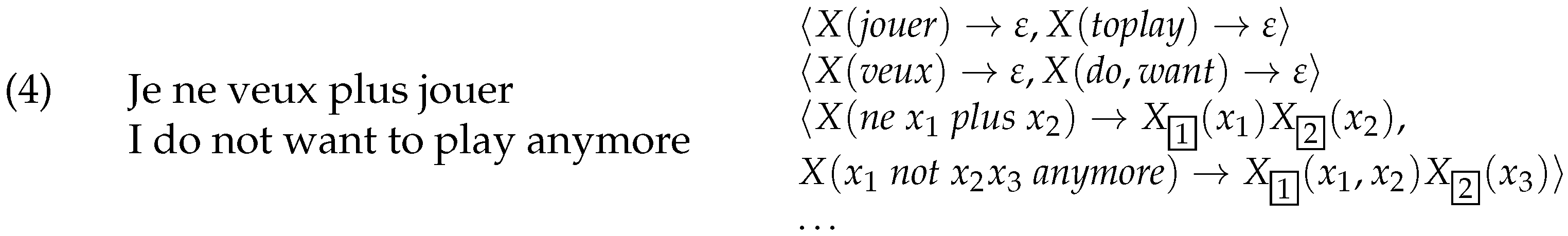Authors of [15,16] use LCFRS for the modeling of such processes. Finally, in machine translation, suitable versions of LCFRS, resp. equivalent formalisms, have been proposed for the modeling of translational equivalence [17,18]. They offer the advantage that certain alignment configurations that cannot be modeled with synchronous variants of CFG can be induced by LCFRS [19]. As an example, see Figure 3, which shows an English sentence with its French translation, along with a grammar that models the alignment between both.

Parsing is a key task since it serves as a backend in many practical applications such as the ones mentioned above. The parsing of LCFRS has received attention both on the symbolic and on the probabilistic side. Symbolic parsing strategies, such as CYK and Earley variants have been presented [20,21,22], as well as automaton-based parsing [23] and data-driven probabilistic parsing techniques [24,25,26]. To our knowledge, however, no LR strategy for LCFRS has so far been presented in the literature. LR parsing is an incremental shift-reduce parsing strategy in which the transitions between parser states are guided by an automaton which is compiled offline. LR parsers were first introduced for deterministic context-free languages [27] and later generalized to context-free languages [28,29] and tree-adjoining languages [30,31]. Also for conjunctive grammars and boolean grammars, LR parsing algorithms exist [32,33,34]. In this paper, we present an LR-style parser for LCFRS, extending our earlier work [35]. Our parsing strategy is based on the incremental parsing strategy implemented by Thread Automata [23].

The remainder of the article is structured as follows. In the following section, we introduce LCFRS and thread automata. Section 3 introduces LR parsing for the context-free case. Section 4 presents the LR algorithm for LCFRS along with an example. In particular, Section 4.1 gives the intuition behind the algorithm, Section 4.2 introduces the algorithms for automaton and parse table constructions, and Section 4.3 presents the parsing algorithm. Section 5 concludes the article.

2. Preliminaries

2.1. Linear Context-Free Rewriting Systems

We now introduce Linear Context-Free Rewriting Systems (LCFRS). In LCFRS, a single non-terminal can span $k\ge 1$ continuous blocks of a string. A CFG is simply a special case of an LCFRS in which $k=1$. We notate LCFRS with the syntax of Simple Range Concatenation Grammars (SRCG) [36], a formalism equivalent to LCFRS. Note that we restrict ourselves to the commonly used string rewriting version of LCFRS and omit the more general definition of LCFRS of [37]. Furthermore, we assume that our LCFRSs are monotone (see condition 3 below) and ε-free (we can make this assumption without loss of generality see [20,38]).

Definition 1 (LCFRS). 

An Linear Context-Free Rewriting System (LCFRS) [1,20] is a tuple $G=(N,T,V,P,S)$ where

• N is a finite set of non-terminals with a function dim: $N\to \mathbb{N}$ determining the fan-out of each $A\in N$;
• T and V are disjoint finite sets of terminals and variables;
• $S\in N$ is the start symbol with $\mathit{dim}\left(S\right)=1$; and
• P is a finite set of rewriting rules (or productions). For all $\gamma \in P$, the following holds.

  • γ has the form

    $$A({\alpha }_0,\dots ,{\alpha }_{\mathit{dim}\left(A\right)-1})\to A_1(x_0^{\left(1\right)},\cdots ,x_{\mathit{dim}\left(A_1\right)-1}^{\left(1\right)})\cdots A_m(x_0^{\left(m\right)},\cdots ,x_{\mathit{dim}\left(A_m\right)-1}^{\left(m\right)})$$

    where $A,A_1,\cdots ,A_m\in N$, $m\ge 0$ being the rank of γ; $x_j^{\left(l\right)}\in V$ for $1\le l\le m,0\le j<\mathit{dim}\left(A_i\right)$; and ${\alpha }_i\in {(V\cup T)}^{+}$ for $0\le i<\mathit{dim}\left(A\right)$; all ${\alpha }_i$ and $x_j^{\left(l\right)}$ are called arguments or components. γ may be abridged as $A\left(\overrightarrow{\alpha }\right)\to A_1\left(\overrightarrow{x_1}\right)\cdots A_m\left({\overrightarrow{x}}_m\right)$; and we define $\mathit{rank}\left(\gamma \right)=m$.
  • For all $x\in V$ there is at most one unique occurrence of x on each lefthand side and righthand side of γ; furthermore, there exists an lefthand side occurrence iff there exists a righthand side occurrence.
  • Variable occurrences in γ are ordered by a strict total order ≺ which is such that for all $x_1,x_2$ with occurrences in γ, if $x_1$ precedes $x_2$ in any ${\overrightarrow{x}}_i$, $1\le i\le m$, then $x_1$ also precedes $x_2$ in α.

The rank of G is given by $\max \left(\right\{\mathit{rank}\left(\gamma \right)\mid \gamma \in P\left\}\right)$ and written as $\mathit{rank}\left(G\right)$. G is of fan-out k if $k\ge \max \left(\right\{\mathit{dim}\left(V\right)\mid V\in N\left\}\right)$ and is written as $\mathit{dim}\left(G\right)$. The set ${\mathcal{C}}_G$ is defined as ${\mathcal{C}}_G={\bigcup }_{\gamma \in P}{\mathcal{C}}_{\gamma }$ (subscript G can be omitted if clear from the context).

The LCFRS derivation is based on the instantiation of rules, the replacement of variable occurrences by strings of terminals.

Definition 2 (Instantiation). 

An instantiation of a production $\gamma \in P$ with $\gamma =A\left(\overrightarrow{\alpha }\right)\to A_1\left({\overrightarrow{\alpha }}_1\right)\cdots A_m\left({\overrightarrow{\alpha }}_m\right)$ is given by a function ${\sigma }_{\gamma }:V_{\gamma }\to T^{*}$, where $V_{\gamma }=\{x\mid \exists i,j such that \mathit{rhs}(\gamma ,i,j)=x\}$ the set of all $x\in V$ occurring in γ. γ is instantiated if all variable occurrences x have been replaced by ${\sigma }_{\gamma }\left(x\right)$. A non-terminal in an instantiated production is an instantiated non-terminal.

We now describe the LCFRS derivation process. A (partial) derivation is specified as a pair $[D:A\left(\overrightarrow{\alpha }\right)]$ called item. Thereby, $A\left(\overrightarrow{\alpha }\right)$ specifies the yield and D is the derivation tree. We use a bracketed representation of trees, e.g., ${\gamma }_0\left({\gamma }_1{\gamma }_2\right)$ is a tree with a root node labeled ${\gamma }_0$ that has two daughters, a left daughter labeled ${\gamma }_1$ and a right daughter labeled ${\gamma }_2$.

Definition 3 (Derivation). 

Let $G=(N,T,V,P,S)$ be an LCFRS. The set ${\mathrm{\Delta }}_G$ of derivable items with respect to G contains all and only those items that can be deduced with the following deduction rules (the subscript G on ${\mathrm{\Delta }}_G$ may be omitted if clear from the context).

• $\frac{}{[\gamma :A\left(\overrightarrow{\alpha }\right)]}\gamma :A\left(\overrightarrow{\alpha }\right)\to \epsilon \in Pand L\left(v\right)=\gamma$
• $\frac{[D_1:A_1\left({\overrightarrow{\alpha }}_1\right)]\cdots [D_m:A_m\left({\overrightarrow{\alpha }}_m\right)]}{[\gamma (D_1\cdots D_m):A\left(\overrightarrow{\alpha }\right)]}A\left(\overrightarrow{\alpha }\right)\to A_1\left({\overrightarrow{\alpha }}_1\right)\cdots A_m\left({\overrightarrow{\alpha }}_m\right)\mathrm{is\; an\; instantiation\; of}\gamma \in P$

We can now define the string language of an LCFRS G on the basis of the yield of a non-terminal.

Definition 4 (Yield, String Language, and Tree Language). 

Let $G=(N,T,V,P,S)$ be an LCFRS.

• For every $A\in N$ we define $\mathit{yield}\left(A\right)=\{\overrightarrow{\alpha }\mid \exists Dsuchthat[D:A\left(\overrightarrow{\alpha }\right)]\in {\mathrm{\Delta }}_G\}$.
• The string language of G is defined as $L_S\left(G\right)=\{w\mid \langle w\rangle \in \mathit{yield}\left(S\right)\}$.
• The derivation tree language of G is defined as $L_D\left(G\right)=\{D\mid \exists wsuchthat[D:S\left(\langle w\rangle \right)]\in {\mathrm{\Delta }}_G\}$.

Note that this definition of a tree language captures the set of derivation trees, not the derived trees with crossing branches along the lines of Figure 1 and Figure 2.

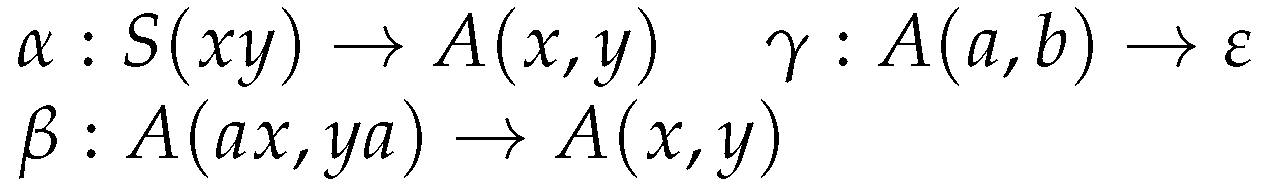
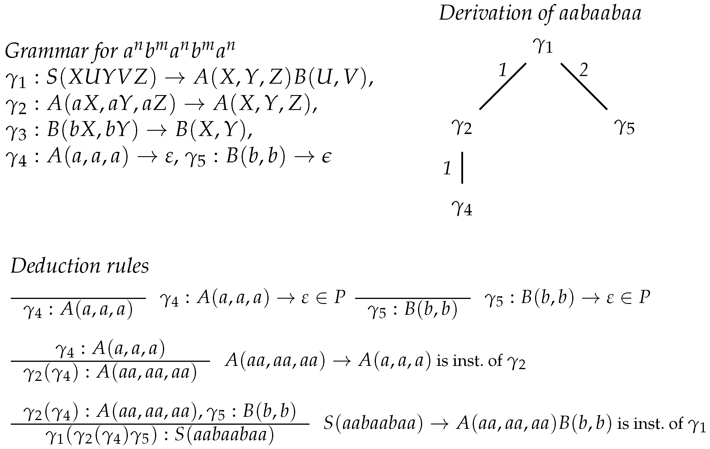
Example 1 (LCFRS Derivation). 

Figure 4 shows an LCFRS that generates the language $a^n{b}^m{a}^n{b}^m{a}^n$, $n,m\in \mathbb{N}$, together with a derivation of the string $aabaabaa$. The derivation works as follows. First, the leaf nodes of the derivation tree are produced using the first deduction rule with the productions ${\gamma }_4$ and ${\gamma }_5$. They introduce the first three as and the two bs. In order to insert three more as, we use the second deduction rule with production ${\gamma }_2$. This leads to a derivation tree with a root labeled ${\gamma }_2$ that has the ${\gamma }_4$ node as its single daughter. Finally the as and the bs are combined with the second deduction rule and production ${\gamma }_1$. This leads to a derivation tree with root label ${\gamma }_1$ that has two daughters, the first one is the ${\gamma }_2$-derivation tree and the second one the ${\gamma }_5$ node. The order of the daughters reflects the order of elements in the righthand sides of productions.

Finally, we define some additional notation that we will need later: Let $\gamma =A({\alpha }_0,\dots ,{\alpha }_{\mathit{dim}\left(A\right)-1})\to A_1(x_0^{\left(1\right)},\cdots ,x_{\mathit{dim}\left(A_1\right)-1}^{\left(1\right)})\cdots A_m(x_0^{\left(m\right)},\cdots ,x_{\mathit{dim}\left(A_m\right)-1}^{\left(m\right)})$ be a production.

• $\mathit{lhs}\left(\gamma \right)$ gives A, $\mathit{lhs}(\gamma ,i)$ gives ${\alpha }_i$ and $\mathit{lhs}(\gamma ,i,j)$ the jth symbol of ${\alpha }_i$; $\mathit{rhs}(\gamma ,l)$ gives $A_l$, and $\mathit{rhs}(\gamma ,l,k)$ gives the kth component of the lth RHS element. Thereby, i, j and k start with index 0, and l starts with index 1. These functions have value ⊥ whenever there is no such element.
• In the sense of dotted productions, we define a set of symbols ${\mathcal{C}}_{\gamma }$ denoting computation points of γ as ${\mathcal{C}}_{\gamma }=\{{\gamma }_{i.j}\mid 0\le i<{\mathit{dim}}_A,0\le j\le |{\alpha }_i\left|\right\}$.

2.2. Thread Automata

Thread automata TA [23] are a generic automaton model which can be parametrized to recognize different mildly context-sensitive languages. The TA for LCFRS (LCFRS-TA) implements a prefix-valid top-down incremental parsing strategy similar to the ones of [21,22]. In this paper, we restrict ourselves to introducing this type of TA.

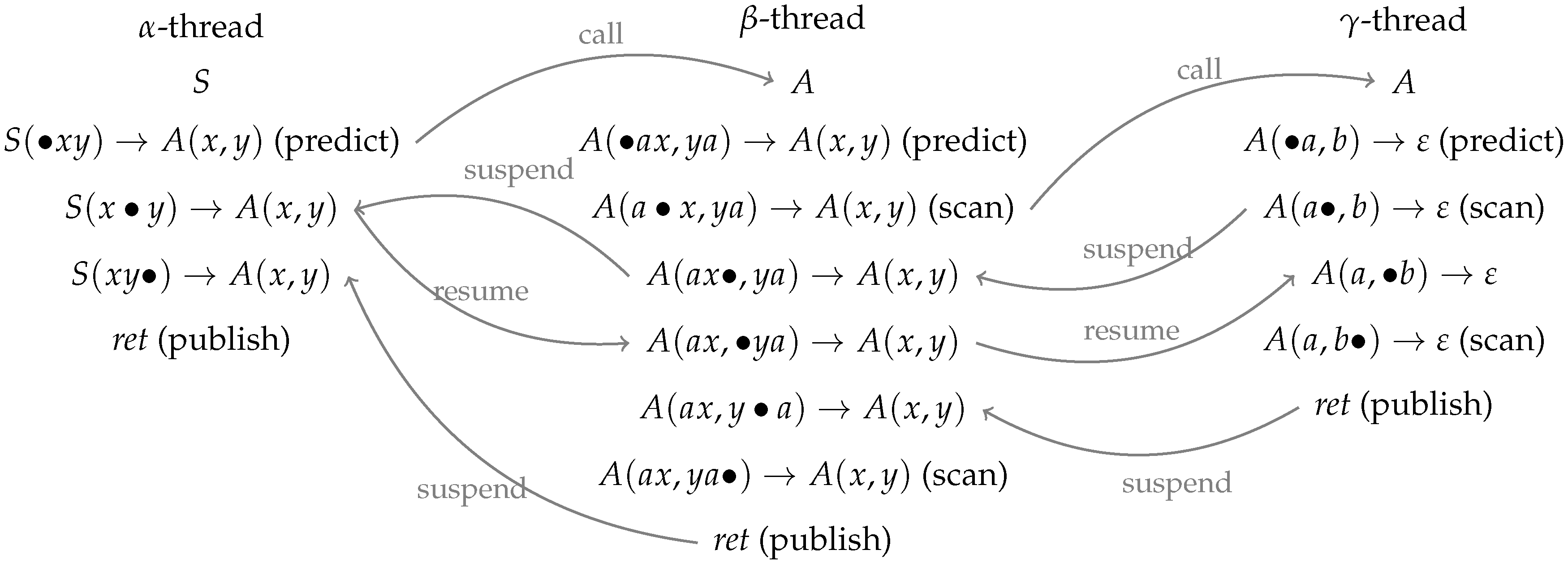
As an example, let us consider the derivation of the word $aaba$ with the LCFRS from Figure 5 and Figure 6 shows a sample run of a corresponding TA where only the successful configurations are given. We have one thread for each rule instantiation that is used in a parse. In our case, the derivation is $S\left(aaba\right)\stackrel{\alpha }{\Rightarrow }A(aa,ba)\stackrel{\beta }{\Rightarrow }A(a,b)\stackrel{\gamma }{\Rightarrow }\epsilon$, we therefore have one thread for the α-rule, one for β and one for γ. The development of these threads is given in the three columns of Figure 6.

Each thread contains at each moment of the TA run only a single symbol, either a non-terminal or a dotted production. The TA starts with the α-thread containing the start symbol. In a predict step, this is replaced with the dotted production corresponding to starting the α-rule. Now the dot precedes the first variable of the non-terminal A in the righthand side. We therefore start a new A-thread (we “call” a new A). In this thread, rule β is predicted, and the dot is moved over the terminal a in a scan step, leading to $A(a•x,ya)\to A(x,y)$ as content of the thread. Now, since the dot again precedes the first component of a righthand side non-terminal A, we call a new A-thread, which predicts γ this time. A scan allows to complete the first component of the γ-rule (thread content $A(a•,b)\to \epsilon$). Here, since the dot is at the end of a component, i.e., precedes a gap, the γ-thread is supended and its mother thread, i.e. the one that has called the γ-thread, becomes the active thread with the dot now moved over the variable for the firsts γ-component ($A(ax•,ya)\to A(x,y)$). Similarly, a second suspend operation leads to the α-thread becoming the active thread again with the dot moved over the finished component of the righthand side A ($S(x•y)\to A(x,y)$). The dot now precedes the variable of the second component of this A, therefore the β-thread is resumed with the dot moving on to the second component ($A(ax,•ya)\to A(x,y)$). Similarly, a second resume operation leads to the γ-thread becoming active with content $A(a,•b)\to \epsilon$. The subsequent scan yields a completed A-item that can be published, which means that the mother thread becomes active with the dot moved over the variable for the last righthand side component. After another scan, again, we have a completed item and the α-thread becomes active with a content $S(xy•)\to A(x,y)$ that signifies that we have found a complete S-yield. Since the entire input has been processed, the TA run was successful and the input is part of the language accepted by the TA.

More generally, an LCFRS-TA for some LCFRS $G=(N,T,V,P,S)$ works as follows. As we have seen, the processing of a single instantiated rule is handled by a single thread which will traverse the lefthand side arguments of the rule. A thread is given by a pair $p:X$, where $p\in {\{1,\dots ,m\}}^{*}$ with m the rank of G is the address, and $X\in N\cup \left\{\mathit{ret}\right\}\cup \mathcal{C}$ where $\mathit{ret}\notin N$ is the content of the thread. In our example in Figure 6, addresses were left aside. They are, however, crucial for determining the mother thread to go back to in a suspend step. In Figure 6, the α-thread has address ε, the β-thread address 1 and the γ-thread address 11, i.e., the address of the mother thread is a prefix of the address of the child thread, respectively. This is why a thread knows where to go back to in a suspend step. An automaton state is given by a tuple $\langle i,p,\mathcal{T}\rangle$ where $\mathcal{T}$ is a set of threads, the thread store, p is the address of the active thread, and $i\ge 0$ indicates that i tokens have been recognized. We use $\langle 0,\epsilon ,\{\epsilon :S\}\rangle$ as start state.

Definition 5 (LCFRS-TA). 

Let $G=(N,T,V,P,S)$ be a LCFRS. The LCFRS thread automaton for G is a tuple $\langle N^{\prime },T,S,\mathit{ret},\delta ,\Theta \rangle$ with

• $N^{\prime }=N\cup {\mathcal{C}}_G\cup \left\{ret\right\}$;
• δ is a function from $\mathcal{C}$ to $\{1,\cdots ,m\}\cup \left\{\perp \right\}$ such that $\delta \left({\gamma }_{k,i}\right)=j$ if there is a l such that $\mathit{lhs}(\gamma ,k,i)=\mathit{rhs}(\gamma ,j-1,l)$, and $\delta \left({\gamma }_{k,i}\right)=\perp$ if $\mathit{lhs}(\gamma ,k,i)\in T\cup \left\{\perp \right\}$; and
• Θ is a finite set of transitions as defined below.

Intuitively, a δ value j tells us that the next symbol to process is a variable that is an argument of the j-th righthand side non-terminal.

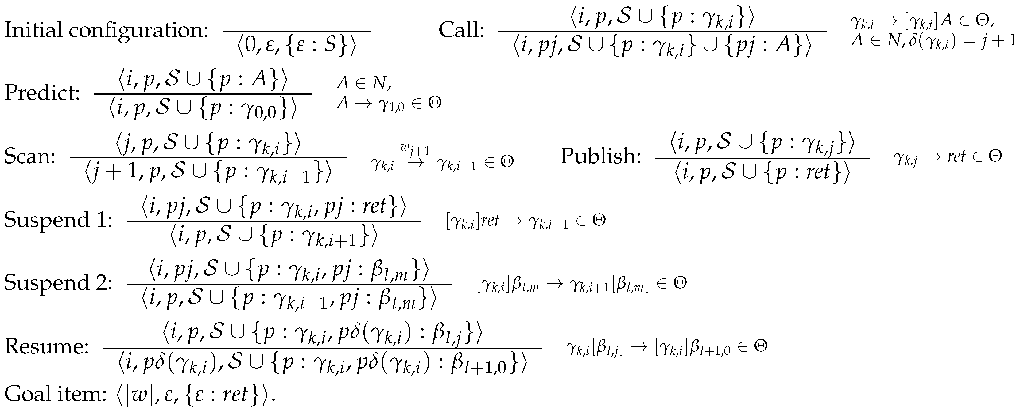
Definition 6 (Transitions of a LCFRS-TA). 

The transition set Θ of a LCFRS-TA as in Definition 5 contains the following transitions:

• Call: ${\gamma }_{k,i}\to \left[{\gamma }_{k,i}\right]A\in \Theta$ if $A=\mathit{rhs}(\gamma ,j-1)$ and $\mathit{lhs}(\gamma ,k,i)=\mathit{rhs}(\gamma ,j-1,0)$ where $j=\delta \left({\gamma }_{k,i}\right)$.
• Predict: $A\to {\gamma }_{0,0}\in \Theta$ if $A=\mathit{lhs}\left(\gamma \right)$.
• Scan: ${\gamma }_{k,i}\stackrel{\mathit{lhs}(\gamma ,k,i)}{\to }{\gamma }_{k,i+1}\in \Theta$ if $\mathit{lhs}(\gamma ,k,i)\in T$.
• Publish: ${\gamma }_{k,j}\to \mathit{ret}\in \Theta$ if $\mathit{dim}\left(\mathit{lhs}\right(\gamma \left)\right)=k+1$ and $j=\left|\mathit{lhs}\right(\gamma ,k\left)\right|$.
• Suspend:

  (i)

  $\left[{\gamma }_{k,i}\right]\mathit{ret}\to {\gamma }_{k,i+1}\in \Theta$ if $\mathit{lhs}(\gamma ,k,i)=\mathit{rhs}(\gamma ,\delta \left({\gamma }_{k,i}\right)-1,\mathit{dim}\left(\mathit{rhs}(\delta \left({\gamma }_{k,i}\right)-1)\right)-1)$.

  (ii)

  $\left[{\gamma }_{k,i}\right]{\beta }_{l,j}\to {\gamma }_{k,i+1}\left[{\beta }_{l,j}\right]\in \Theta$ if $\mathit{dim}\left(\mathit{lhs}\right(\beta \left)\right)>l+1$, $\left|\mathit{lhs}\right(\beta ,l\left)\right|=j$, $\mathit{lhs}(\gamma ,k,i)=\mathit{rhs}(\gamma ,\delta \left({\gamma }_{k,i}\right)-1,l)$ and $\mathit{rhs}(\gamma ,\delta \left({\gamma }_{k,i}\right)-1)=\mathit{lhs}\left(\beta \right)$.

• Resume: ${\gamma }_{k,i}\left[{\beta }_{l,j}\right]\to \left[{\gamma }_{k,i}\right]{\beta }_{l+1,0}\in \Theta$ if $\mathit{lhs}(\gamma ,k,i)=\mathit{rhs}(\gamma ,\delta \left({\gamma }_{k,i}\right)-1,l+1)$, $\mathit{rhs}(\gamma ,\delta \left({\gamma }_{k,i}\right)-1)=\mathit{lhs}\left(\beta \right)$ and ${\beta }_{l,j+1}\notin {\mathcal{C}}_G$.

These are all thransitions in Θ.

A transition $\alpha \stackrel{a}{\to }\beta$ roughly indicates that in the current thread store, α can be replaced with β while scanning a. Square brackets in α and β indicate parts that do not belong to the active thread. Call transitions start a new thread for a daughter non-terminal, i.e., a righthand side non-terminal. They move down in the parse tree. Predict transitions predict a new rule for a non-terminal A. Scan transitions read a lefthand side terminal while scanning the next input symbol. Publish marks the completion of a production, i.e., its full recognition. Suspend transitions suspend a daughter thread and resume the parent. i.e., move up in the parse tree. There are two cases: Either (i) the daughter is completely recognized (thread content $\mathit{ret}$) or (ii) the daughter is not yet completely recognized, we have only finished one of its components. Resume transitions resume an already present daughter thread, i.e., move down into some daughter that has already been partly recognized.

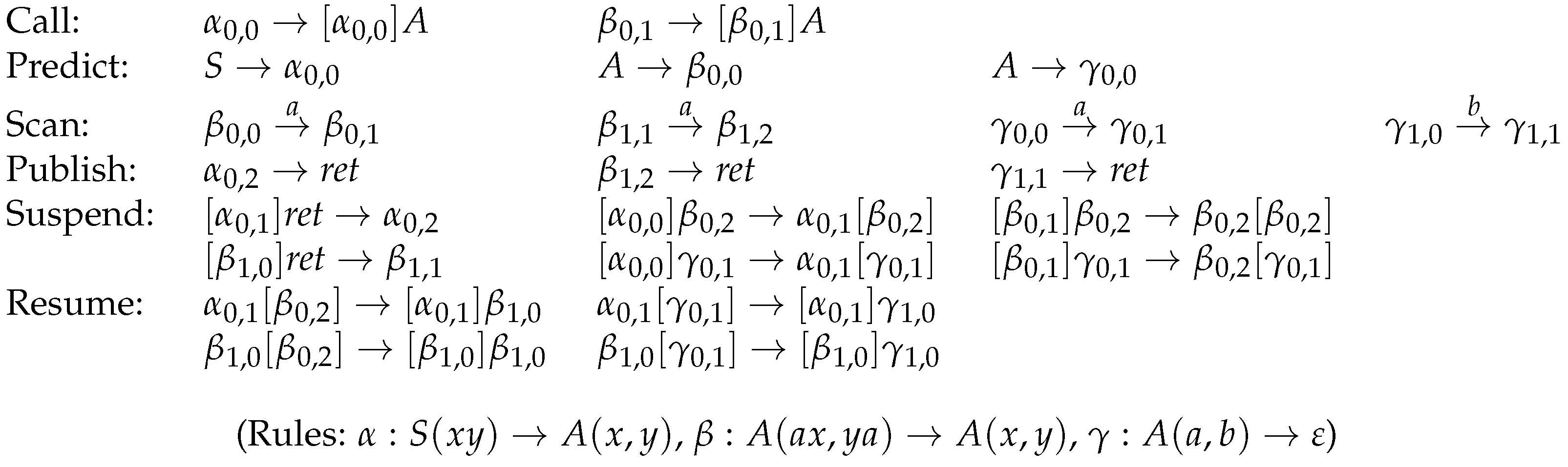
Figure 7 shows the transitions for our sample grammar. Let us explain the semantics of these rules with these examples before moving to the general deduction rules for TA configurations. As already mentioned, a rule $X_1\stackrel{t}{\to }{X}_2$ with $X_1,X_2\in N^{\prime }$ and $t\in T\cup \left\{\epsilon \right\}$ expresses that with $X_1$ being the content of the active thread, we can replace $X_1$ with $X_2$ while scanning t. The predict, scan and publish rules are instances of this rule type. $X\in N^{\prime }$ in square brackets to the left characterize the content of the mother of the active thread while $X\in N^{\prime }$ in square brackets to the right characterize the content of a daughter thread where the address of the daughter depends on the one of the active thread and the δ-value of the content of the active thread. Consider for instance the last suspend rule. It signifies that if the content of the active thread is ${\gamma }_{0,1}$ and its mother thread has content ${\beta }_{0,1}$, this mother thread becomes the new active thread with its content changed to ${\beta }_{0,2}$ while the daughter thread does not change content. The resume rules, in contrast to this, move from the active thread to one of its daughters. Take for instance the last rule. It expresses that, if the active thread has content ${\beta }_{1,0}$ and if this thread has a $\delta \left({\beta }_{1,0}\right)$th daughter thread with content ${\gamma }_{0,1}$, we make this daughter thread the active one and change its content to ${\gamma }_{1,0}$, i.e., move its dot over a gap.

This is not exactly the TA for LCFRS proposed in [23] but rather the one from [39], which is close to the Earley parser from [21].

The set of configurations for a given input $w\in T^{*}$ is then defined by the deduction rules in Figure 8 (the use of set union ${\mathcal{S}}_1\cup {\mathcal{S}}_2$ in these rules assumes that ${\mathcal{S}}_1\cap {\mathcal{S}}_2=\varnothing$). The accepting state of the automaton for some input w is $\langle \left|w\right|,\epsilon ,\{\epsilon :ret\}\rangle$.

3. LR Parsing

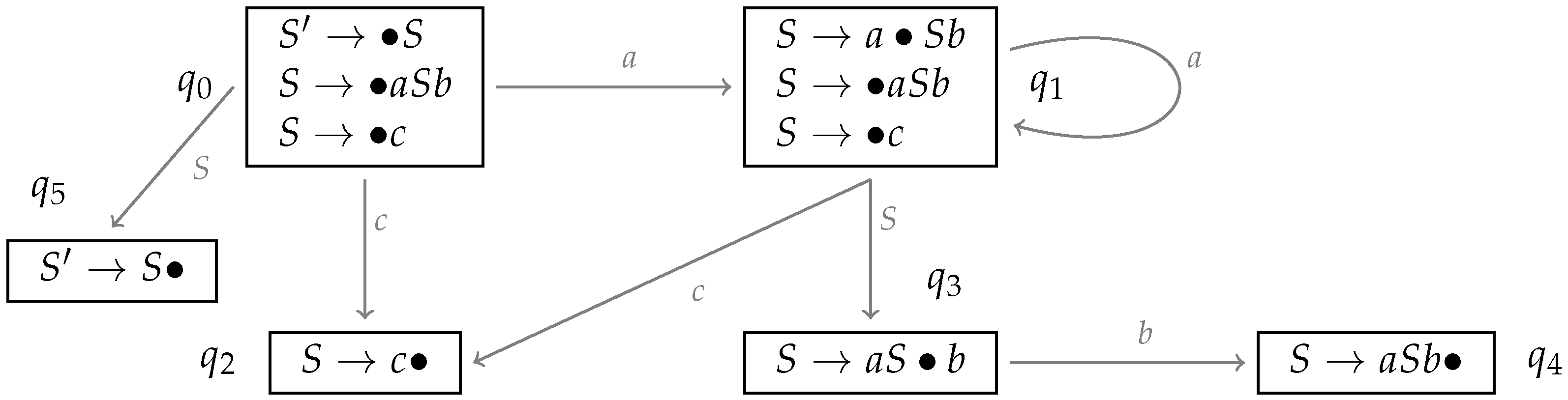
In an LR parser (see [40] chapter 9), the parser actions are guided by an automaton, resp. a parse table which is compiled offline. Consider the context-free case. An LR parser for CFG is a guided shift-reduce parser, in which we first build the LR automaton. Its states are sets of dotted productions closed under prediction, and its transitions correspond to having recognized a part of the input, e.g., to moving the dot over a righthand side element after having scanned a terminal or recognized a non-terminal.

Consider for instance the CFG $G=\langle \left\{S\right\},\{a,b,c\},\{S\to aSb|c\},S\rangle$. Its LR automaton is given in Figure 9. The construction of this automaton starts from the prediction closure of $\{S^{\prime }\to •S\}$, which contains the two S-productions with the dot at the beginning of the righthand side. The prediction closure of a set of dotted productions q is defined as follows: if $A\to \alpha •B\beta \in q$, then $B\to •\gamma \in q$ for all B-productions $B\to \gamma$ in the grammar. From a state q, a new state can be obtained by computing all items that can be reached by moving the dot over a certain $x\in N\cup T$ in any of the dotted productions in q and then, again, building the prediction closure. The new state can be reached from the old one by an edge labeled with x. This process is repeated until all possible states have been constructed. In our example, when being in $q_0$, we can for instance reach $q_1$ by moving the dot over an a, and we can reach $q_5$ (the acceptance state) by moving the dot over an S.

This automaton guides the shift-reduce parsing in the following way: At every moment, the parser is in one of the states. We can shift an $a\in T$ if there is an outgoing a-transition. The state changes according to the transition. We can reduce if the state contains a completed $A\to \alpha •$. We then reduce with $A\to \alpha$. The new state is obtained by following the A-transition, starting from the state reached before processing that rule.

The information about possible shift and reduce operations in a state is precompiled into a parse table: Given an LR automaton with n states, we build a parse table with n rows. Each row i, $0\le i<n$, describes the possible parser actions associated with the state $q_i$, i.e., for each state and each possible shift or reduce operation, it tells us in which state to go after the operation. The table has $\left|T\right|+\left|N\right|+1$ columns where the first are indexed with the terminals, then follows a column for reduce operations and then a column for each of the non-terminals. For every pair of states $q_i$, $q_j$ that are linked by an a-edge for some $a\in T$, the field of $q_i$ and a contains sj, which indicates that in $q_i$, one can shift an a and then move to $q_j$. For every state $q_i$ that contains rule number j with a dot at the end of the righthand side, we add rj to the reduce field of $q_i$. Finally, for every pair of states $q_i$, $q_j$ that are linked by an A-edge for some $A\in N$, the field of $q_i$ and A contains j, which indicates that in $q_i$, after having completed an A, we can move to $q_j$. 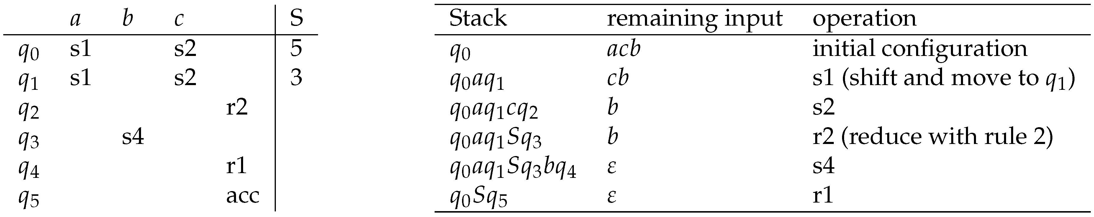On the left of Figure 10, we see the parse table resulting from the automaton in Figure 9. The first $\left|T\right|+1$ columns are the so-called action-part of the table while the last $\left|N\right|$ columns form the goto-part.

The parse table determines the possible reductions and shifts we can do at every moment. We start parsing with a stack containing only $q_0$. In a shift, we push the new terminal followed by the state indicated in the table on the stack. In a reduction, we use the production indicated in the table. We pop its righthand side (in reverse order) and push its lefthand side onto the stack. The new state is the state indicated in the parse table field for the state preceding the lefthand side of this production on the stack and the lefthand side category of the production. On the right of Figure 10, we see a sample trace of a parse according to our LR parse table. Note that this example allowed for deterministic LR parsing, which is not the case in general. There might be shift-reduce or reduce-reduce conflicts.

4. LR for LCFRS

4.1. Intuition

We will now adapt the ideas underlying LR parsing for CFG to the case of LCFRS. The starting point is the set of possible threads that can occur in a TA for a given LCFRS. Our LR automaton for LCFRS precompiles predict, call and resume steps into single states, i.e., states are closed under these three operations.

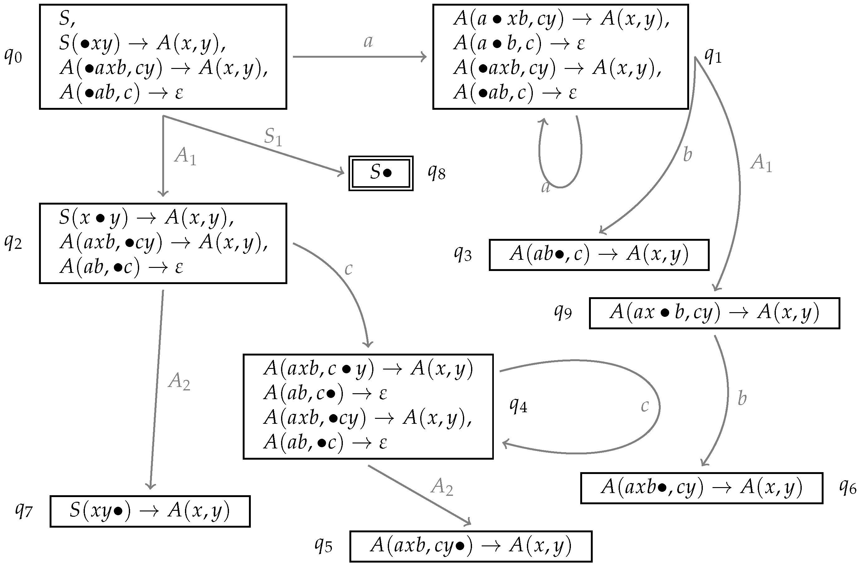
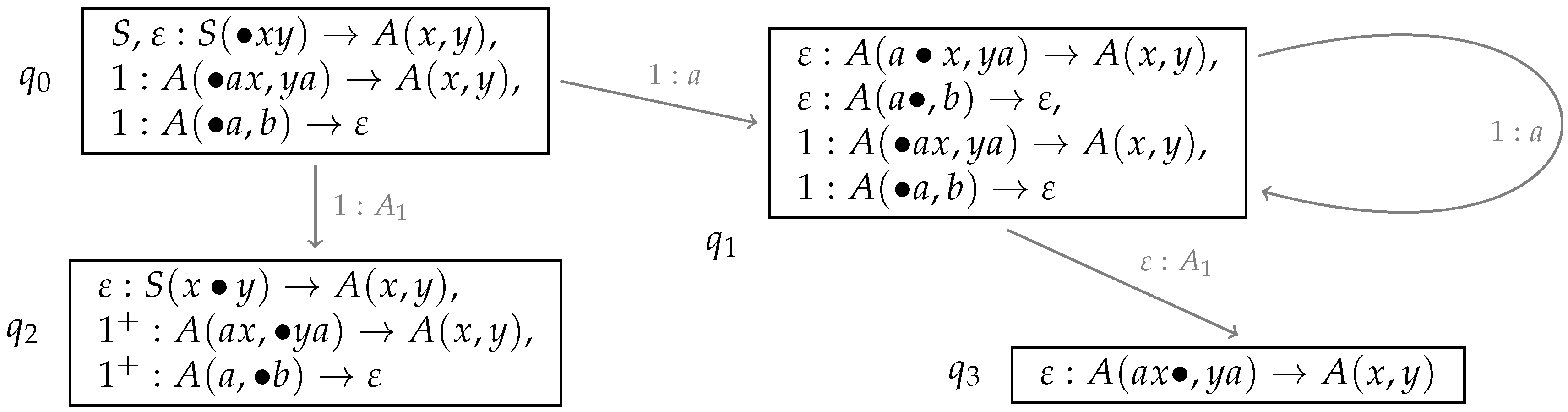
As an example, consider the TA from Section 2.2. Figure 11 sketches some of the states one obtains for this TA.

As in the CFG case, we start with a state for the start symbol S and, in this state, add all predictions of S-rules with the dot at the left of the lefthand side component. Furthermore, for every item in some state q where the dot precedes a variable: If this variable is the ith component of a righthand side non-terminal A, we add to q all A-rules with the dot at the beginning of the ith component in the lefthand side. For $i=1$, this is a call-and-predict operation, for $i>1$ a resume operation.

Moving the dot over a terminal symbol a leads to a transition labeled with a that yields a new state. And moving the dot over the variable that is the ith component of some righthand side symbol A leads to a transition labeled with $A_i$.

Our parser then has shift operations and two kinds of reduce operations (the two types of suspend operations in the TA). Either we reduce the ith component of some A where $i<\mathit{dim}\left(A\right)$ or we reduce the last component of some A. In the first case, we have to keep track of the components we have already found, in particular of their derivation tree addresses. This is why we have to extend the states sketched in Figure 11 to using dotted productions with addresses.

Our predict/resume closure operations then have to add the index of the daughter that gets predicted/resumed to the address. A problem here is that this can lead to states containing infinitely many items. An example is $q_2$ in Figure 11. The dotted production $A(ax,•ya)\to A(x,y)$ leads, via the resume closure, to new instances of $A(ax,•ya)\to A(x,y)$ and $A(a,•b)\to \epsilon$, this time with a different address since these are daughters of the first. Consequently, $q_2$ would be the set $\{\epsilon :S(x•y)\to A(x,y)$, $1:A(ax,•ya)\to A(x,y)$, $1:A(a,•b)\to \epsilon$, $11:A(ax,•ya)\to A(x,y)$, $11:A(a,•b)\to \epsilon$, $111:A(ax,•ya)\to A(x,y)$, $111:A(a,•b)\to \epsilon$, ...}. Such a problem of an infinite loop of predict or resume steps occurs whenever there is a left recursion in one of the components of a rule. We do not want to exclude such recursions in general. Therefore, in order to keep the states finite nevertheless, we allow the addresses to be regular expressions. Then $q_2$ for instance becomes $\{\epsilon :S(x•y)\to A(x,y)$, $1^{+}:A(ax,•ya)\to A(x,y)$, $1^{+}:A(a,•b)\to \epsilon \}$. 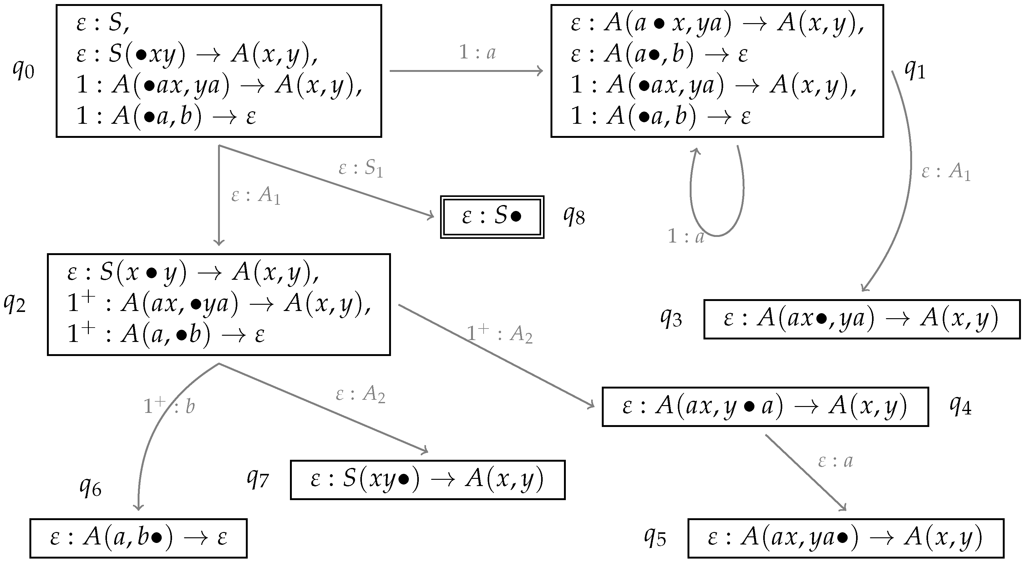Concerning the transitions, here as well, we add the addresses of the item(s) that have triggered that transition. See Figure 12 for an example. A new state always starts with an item with address ε.

Once the automaton is constructed, the shift-reduce parser proceeds as follows: A configuration of the parser consists of a stack, a set of completed components and the remaining input. The completed components are of the form $r\boxed{k}{\gamma }_i$ where r is a regular expression, $\boxed{k}$ is a pointer to the derivation tree node for this use of the rule $\gamma :A(a,b)\to \epsilon$ and i is the component index. The stack has the form ${\mathrm{\Gamma }}_1{x}_1{\mathrm{\Gamma }}_2\cdots x_{n-1}{\mathrm{\Gamma }}_n$ where ${\mathrm{\Gamma }}_i$ is a regular expression followed by a state and $x_i\in T\cup \left\{{\boxed{j}}_k\right|\boxed{j}$ points at a derivation tree node for a rule γ with $1\le k\le \mathit{dim}\left(\mathit{lhs}\right(\gamma \left)\right)\}$.

For the input $aaba$ for instance, we would start with a stack $\epsilon q_0$ and then, following the corresponding transition in the automaton, we can shift an a and move to $q_1$. Since the shift transition tells us that this shift refers to the daughter with address 1, this address is concatenated to the preceding address. The new stack would be $\epsilon q_{0}a1q_1$ and, after a second shift, $\epsilon q_{0}a1q_{1}a11q_1$. In $q_1$ we can not only shift as but we can also reduce since there is an item with the dot at the end of the first A-component, $A(a•,b)\to \epsilon$. Such a reduce means that we remove this component (here a single a) from the stack, then create a node $11\boxed{0}{\gamma }_1$ as part of the set of completed components, and then push its pointer and index (here ${\boxed{0}}_1$). The transition from the state preceding the a that is labeled $\mathit{lhs}{\left(\gamma \right)}_1$ gives the new state and address. The stack is then $\epsilon q_{0}a1q_1{\boxed{0}}_{1}1q_3$, and the set of completed components is $\left\{11\boxed{0}{\gamma }_1\right\}$. $q_3$ also tells us that a first component of a rule, this time $A(ax,ya)\to A(x,y)$, has been completed. It consists of a followed by a first A-component, therefore we have to remove a and ${\boxed{0}}_1$ (in reverse order) from the stack and then follow the $A_1$ transition from $q_0$. The result is a stack $\epsilon q_0{\boxed{1}}_{1}1q_2$ and a completed components set $\{1\boxed{1}{\beta }_1,11\boxed{0}{\gamma }_1\}$. The completed components are, furthermore, equipped with an immediate dominance relation. In this example, $\boxed{1}$ immediately dominates $\boxed{0}$. Whenever a reduce state concerns a component that is not the first one, we check in our set of completed components that we have already found a preceding component with the same address or (if it is a regular expression denoting a set) a compatible address. In this case, we increment the component index of the corresponding derivation tree node. In the end, in case of a successful parse, we have a stack $\epsilon q_0{\boxed{i}}_1\epsilon q_{\mathit{acc}}$ and a component set giving the entire derivation tree with root node $\boxed{i}$.

4.2. Automaton and Parse Table Construction

The states of the LR-automaton are sets of pairs $r:X$ where r is a regular expression over $\{1,\cdots ,\mathit{rank}(G\left)\right\}$, and $X\in {\mathcal{C}}_G\cup \left\{S\right\}$. They represent predict and resume closures.

Definition 7. 

We define the predict/resume closure $\overline{q}$ of some set $q\subseteq \{\epsilon :X|X\in {\mathcal{C}}_G\cup \left\{S\right\}\}$ by the following deduction rules:

• Initial predict: $\frac{\epsilon :S}{\epsilon :{\alpha }_{0,0}}\mathit{lhs}\left(\alpha \right)=S$
• Predict/resume: $\frac{p:{\gamma }_{i,j}}{pk:{\gamma }_{l,0}^{\prime }}\mathit{lhs}(\gamma ,i,j)=\mathit{rhs}(\gamma ,k-1,l),\mathit{rhs}(\gamma ,k)=\mathit{lhs}\left({\gamma }^{\prime }\right)$

This closure is not always finite. However, if it is not, we obtain a set of items that can be represented by a finite set of pairs $r:{\gamma }_{i,j}$ plus eventually $\epsilon :S$ such that r is a regular expression denoting a set of possible addresses. As an example for such a case, see $q_2$ in Figure 12. Let ${\mathit{Reg}}_G$ be the set of all regular expressions over $\{1,\cdots ,\mathit{rank}(G\left)\right\}$.

Lemma 8. 

For every $q\subseteq \{\epsilon :X|X\in {\mathcal{C}}_G\cup \left\{S\right\}\}$, it holds that if $\overline{q}$ is infinite, then there is a finite set ${\overline{q}}^{\prime }\subset \{r:X|r\in {\mathit{Reg}}_G,X\in {\mathcal{C}}_G\cup \left\{S\right\}\}$ such that $\overline{q}=\{p:X|thereisanr:X\in {\overline{q}}^{\prime }withp\in L\left(r\right)\}$.

Proof. 

${\mathcal{C}}_G$ is finite. For each ${\gamma }_{i,j}\in {\mathcal{C}}_G$, the set of possible addresses it might be combined with in a state that is the closure of $\{\epsilon :X_1,\epsilon :X_2,\cdots ,\epsilon :X_n\}$ is generated by the CFG $\langle N,T,P,S_{new}\rangle$ with

• $N={\mathcal{C}}_G\cup \left\{S\right\}\cup \left\{S_{new}\right\}$,
• $T=\{1,\cdots ,m\}$, and
• P contains the following rules:

  -

  $S_{new}\to X_i\in P$ for all $1\le i\le n$,

  -

  $X\to Yk\in P$ for all instances $\frac{p:X}{pk:Y}$ of deduction rules,

  -

  and ${\gamma }_{i,j}\to \epsilon$.

This is a regular grammar, its string language can thus be characterized by a regular expression.

The construction of the set of states starts with $q_0=\overline{\{\epsilon :S\}}$. From this state, follwing a-transitions or $A_i$-transitions as sketched above, we generate new states. We first formalize these transitions:

Definition 9. 

Let $G=(N,T,V,P,S)$ be a LCFRS. Let $q\subseteq \{\epsilon :S\}\cup \{r:X|r\in {\mathit{Reg}}_G,X\in {\mathcal{C}}_G\}$.

• For every $A\in N$, every $1\le i\le \mathit{dim}\left(A\right)$ and every $r\in {\mathit{Reg}}_G$, we define

  -

  $\mathit{read}(q,A_i,r)=\{\epsilon :{\gamma }_{j,k+1}|r:{\gamma }_{j,k}\in q$ and there is some l such that $\mathit{rhs}(\gamma ,l)=A$ and $\mathit{lhs}(\gamma ,j,k)=\mathit{rhs}(\gamma ,l,i-1)\}$ and

  -

  $\overline{\mathit{read}}(q,A_i,r)=\overline{\mathit{read}(q,A_i,r)}$.

• For every $a\in T$ and every $r\in {\mathit{Reg}}_G$, we define

  -

  $\mathit{read}(q,a,r)=\{\epsilon :{\gamma }_{j,k+1}|r:{\gamma }_{j,k}\in q$ and $\mathit{lhs}(\gamma ,j,k)=a\}$ and

  -

  $\overline{\mathit{read}}(q,a,r)=\overline{\mathit{read}(q,a,r)}$.

The set of states of our automaton is then the closure of $\left\{q_0\right\}$ under the application of the $\overline{read}$-functions. The edges in our automaton correspond to $\overline{read}$-transitions, where each edge is labeled with the corresponding pair $r:A_i$ or $r:a$ respectively. Furthermore, we add a state $\{\epsilon :S•\}$ and an edge labeled $\epsilon :S_1$ from the start state to this state, which is the acceptance state.

The complete automaton we obtain for the grammar in Figure 5 is shown in Figure 13. For the sake of readability, we use dotted productions instead of the computation points ${\gamma }_{i,j}$.

The number of possible states is necessarily finite since each state is the closure of some set containing only items with address ε. There are only finitely many such sets.

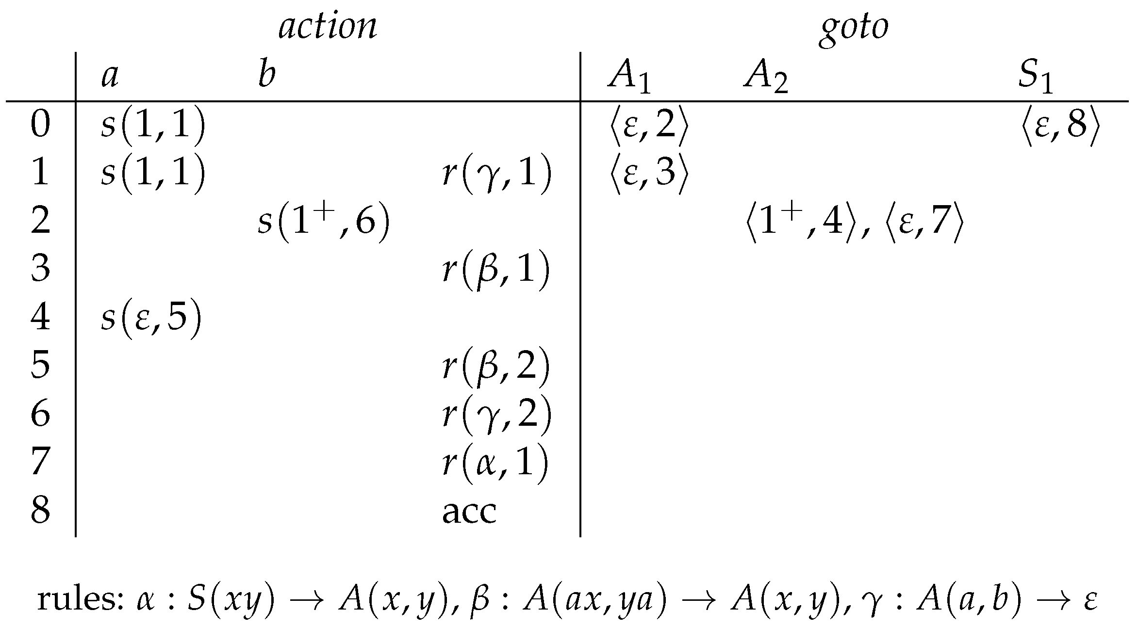
In the parse table, our operations are $s(p,q)$ for shifting some terminal a followed by the old address concatenated with p and state q and $r(\alpha ,i)$ for reducing the ith component of rule α. The two reduce operations can be distinguished by the component indices. These operations are entered into the first $\left|T\right|+1$ columns of the table, the so-called action part. Furthermore, the goto-part of the table tells where to go when traversing a component edge and which address to add then.

The parse table can be read off the automaton as follows:

Definition 10. 

Let $G=\langle N,T,P,S\rangle$ be a LCFRS, M its LR-automaton with state set Q. Then we define the corresponding LR parse table as a pair $\langle \mathit{action},\mathit{goto}\rangle$ with $\mathit{action}$ a $\left|Q\right|\times \left(\right|T|+1)$ table and $\mathit{goto}$ a $\left|Q\right|\times \left|\right\{A_i|A\in N,1\le i\le \mathit{dim}\left(A\right)\}|$ table. The content of these tables is as follows:

• $s(p,q^{\prime })\in \mathit{action}(q,a)$ iff $\overline{\mathit{read}}(q,a,p)=q^{\prime }$;
• $r(\gamma ,i)\in \mathit{action}(q,-)$ iff there is some $p:{\gamma }_{i-1,k}\in q$ such that $k=\left|\mathit{lhs}\right(\gamma ,i-1\left)\right|$.
• $\langle p,q^{\prime }\rangle \in \mathit{goto}(q,A_i)$ iff $\overline{\mathit{read}}(q,A_i,p)=q^{\prime }$.
• Nothing else is in these tables.

Figure 14 shows the parse table for our example.

4.3. Parsing Algorithm

The parser has slightly more complex configurations than the CFG shift-reduce parser. Let Q be the set of states of the LR automaton for a given LCFRS G, $q_0$ the state containing $\epsilon :S$ and $q_{\mathit{acc}}$ the accepting state containing $\epsilon :S•$. Furthermore, let $\mathcal{N}=\{\boxed{0},\boxed{1},\boxed{2},\cdots \}$ be the set of possible pointers to derivation tree nodes. The parser configurations are then triples $\langle \mathrm{\Gamma },C,i\rangle$ consisting of

• a stack $\mathrm{\Gamma }\in {\mathit{Reg}}_G\circ Q\circ {((T\cup \left\{{\boxed{i}}_k\right|\boxed{i}\in \mathcal{N},k\le {\mathit{max}}_{A\in N}\mathit{dim}\left(A\right)\})\circ {\mathit{Reg}}_G\circ Q)}^{*}$,
• a set of constraints C that are either of the form $r\boxed{i}{\gamma }_j$ with $r\in {\mathit{Reg}}_G$, $\boxed{i}\in \mathcal{N}$, $\gamma \in P$ and $1\le j\le \mathit{dim}\left(\mathit{lhs}\right(\gamma \left)\right)$ or of the form $\boxed{k}{⊲}_d\boxed{l}$ with $\boxed{k},\boxed{l}\in \mathcal{N}$, $1\le d\le \mathit{rank}\left(G\right)$.
• and the index j up to which the input w has been recognized, $0\le j\le \left|w\right|$.

Concerning the constraint set C, the first type of constraints describes nodes in the derivation tree while the second describes immediate dominance relations between them, more precisely the fact that one node is the dth daughter of another node. There is an immediate relation between the two: if $\boxed{i_1}{⊲}_d\boxed{i_2}$, then the address of $\boxed{i_2}$ must be the regular expression of $\boxed{i_1}$ concatenated with the daughter index d of $\boxed{i_2}$. Let ${\mathcal{N}}_C$ be the set of indices from $\mathcal{N}$ occurring in C.

The initial configuration is $\langle \epsilon q_0,\varnothing ,0\rangle$. From a current configuration, a new one can be obtained by one of the following operations:

• Shift: Whenever we have $pq$ on top of the stack, the next input symbol is a and in our parse table we have $\mathit{action}(q,a)=s(p^{\prime },q^{\prime })$, we push a followed by $p{p}^{\prime }{q}^{\prime }$ onto the stack and increment the index j.
• Reduce: Whenever the top of the stack is $p_{1}q$ and we have a parse table entry $r(\gamma ,i)\in \mathit{action}(q,-)$, we can reduce the ith component of γ, i.e, suspend γ. Concretely, this means the following:

  -

  Concerning the constraint set C, if $i=1$, we add $p_1\boxed{k}{\gamma }_1$ to C where $\boxed{k}$ is a new pointer.

  -

  If $i\ge 1$, we check whether there is a $p_2\boxed{k}{\gamma }_{i-1}$ in C such that the intersection $L\left(p_1\right)\cap L\left(p_2\right)$ of the languages denoted by $p_1$ and $p_2$, $L\left(p_1\right)$ and $L\left(p_2\right)$, is not empty. We then replace $p_2\boxed{k}{\gamma }_{i-1}$ in C with $p\boxed{k}{\gamma }_i$ where p is a regular expression denoting $L\left(p_1\right)\cap L\left(p_2\right)$.

  -

  Concerning the stack Γ, we remove $3\left|\mathit{lhs}\right(\gamma ,i\left)\right|$ elements (i.e., terminals/component pointers and their regular expressions and states) from Γ. Suppose the topmost state on the stack is now $p^{\prime }{q}^{\prime }$. If $\mathit{goto}(q^{\prime },\mathit{lhs}{\left(\gamma \right)}_i)=\langle p^{″},q^{″}\rangle$, we push ${\boxed{k}}_i$ followed by $p^{\prime }{p}^{″}{q}^{″}$ on the stack.

  -

  Concerning the dominance relations, for every ${\boxed{i}}_j$ among the symbols we removed from the stack, we add $\boxed{k}{⊲}_d\boxed{i}$ where d is the corresponding daughter index.

  -

  It can happen that, thanks to the new dominance relations, we can further restrict the regular expressions characterizing the addresses in C. For instance, if we had $1^{+}\boxed{i}\cdots$, $1^{+}\boxed{k}\cdots$ and $\boxed{i}{⊲}_1\boxed{k}$ in our set, we would replace the address of $\boxed{k}$ with $1^{+}1$.

  -

  The index j remains unchanged in reduce steps.

Note that the intersection of two deterministic finite state automata is quadratic in the size of the two automata. In LCFRS without left recursion in any of the components, the intersection is trivial since the regular expressions denote only a single path each.

As an example, we run the parser from Section 4.2 with an input $w=aaba$. The trace is shown in Figure 15. In this example, the immediate dominance constraints in C are depicted as small trees. We start in $q_0$, and shift two as, which leads to $q_1$. We have then fully recognized the first components of γ and β: We suspend them and keep them in the set of completed components, which takes us to $q_2$. Shifting the b takes us to $q_6$, from where we can reduce, which finally takes us to $q_4$. From there, we can shift the remaining a (to $q_5$), with which we have fully recognized β. We can now reduce both β and with that, α, which takes us to the accepting state $q_8$.

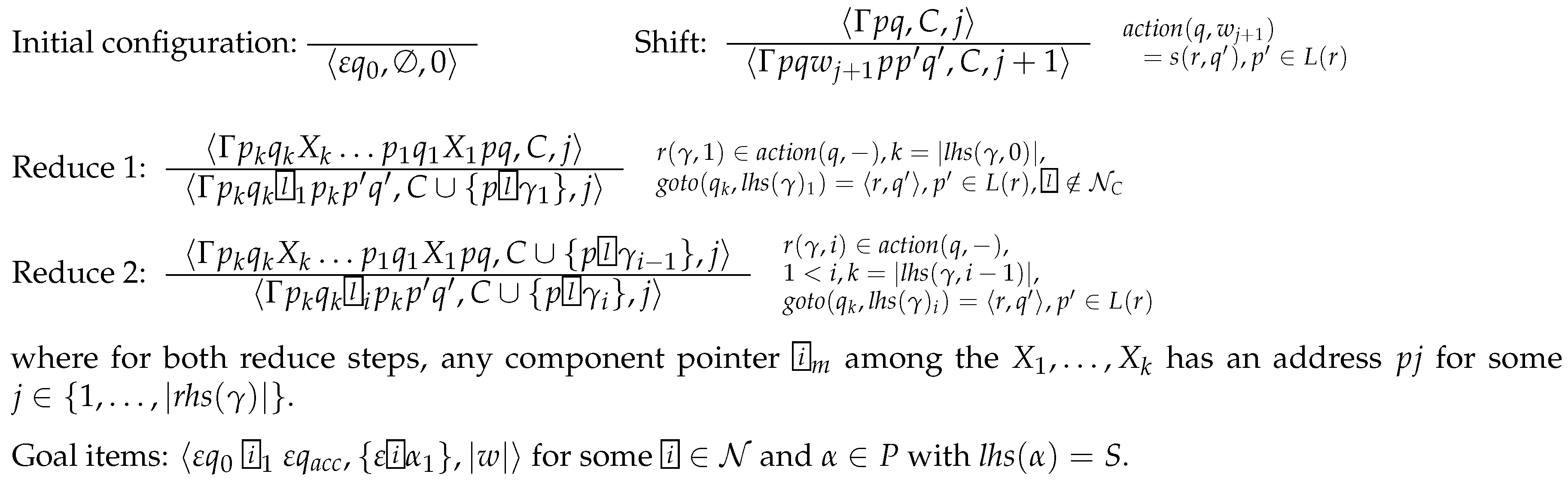
The way the different parsing operations can lead to new configurations can be described by a corresponding parsing schema, i.e., a set of deduction rules and a goal item specification. This is given in the following definition (the use of set union $C_1\cup C_2$ in these rules assumes $C_1\cap C_2=\varnothing$) (comparing the configurations of a LCFRS-TA to the configurations of our parser, it becomes clear that one problem of the TA is that, because of possible call-predict loops, we can have infinitely many configurations in a TA. [23] avoids this problem by a dynamic programming implementation of TAs. In our automata, this problem does not occur because of the regular expressions we use as addresses).

Definition 11 (LR Parsing: Deduction Rules). 

Let $G=\langle N,T,P,S\rangle$ be a LCFRS, $\langle \mathit{action},\mathit{goto}\rangle$ its LR parse table, and $q_0$ and $q_{\mathit{acc}}$ as introduced above.

The set of possible configurations for the LR parser is then defined by the following deduction rules:

• Initial configuration:$\frac{}{\langle \epsilon q_0,\varnothing ,0\rangle }$
• Shift:
  $\frac{\langle \mathrm{\Gamma }pq,C,j\rangle }{\langle \mathrm{\Gamma }pq{w}_{j+1}p{p}^{\prime }{q}^{\prime },C,j+1\rangle }\mathit{action}(q,w_{j+1})=s(p^{\prime },q^{\prime })$
  Reduce 1:
  $\frac{\langle \mathrm{\Gamma }{p}_k{q}_k{X}_k\cdots p_1{q}_1{X}_{1}pq,C,j\rangle }{\langle \mathrm{\Gamma }{p}_k{q}_k{\boxed{l}}_1{p}_k{p}^{\prime }{q}^{\prime },f_{⊲}(C\cup \left\{p\boxed{l}{\gamma }_1\right\}\cup C_{⊲}),j\rangle }\begin{array}{c}r(\gamma ,1)\in \mathit{action}(q,-),k=\left|\mathit{lhs}\right(\gamma ,0\left)\right|,\hfill \\ \mathit{goto}(q_k,\mathit{lhs}{\left(\gamma \right)}_1)=\langle p^{\prime },q^{\prime }\rangle ,\boxed{l}\notin {\mathcal{N}}_C\hfill \end{array}$
  Reduce 2:
  $\frac{\langle \mathrm{\Gamma }{p}_k{q}_k{X}_k\cdots p_1{q}_1{X}_{1}pq,C\cup \left\{p^{″}\boxed{l}{\gamma }_{i-1}\right\},j\rangle }{\langle \mathrm{\Gamma }{p}_k:q_k{\boxed{l}}_i{p}_k{p}^{\prime }{q}^{\prime },f_{⊲}(C\cup \left\{p_{new}\boxed{l}{\gamma }_i\right\}\cup C_{⊲}),j\rangle }\begin{array}{c}r(\gamma ,i)\in \mathit{action}(q,-),1<i,k=\left|\mathit{lhs}\right(\gamma ,i-1\left)\right|,\hfill \\ A=\mathit{lhs}\left(\gamma \right),\mathit{goto}(q_k,A_i)=\langle p^{\prime },q^{\prime }\rangle ,\hfill \\ L\left(p_{new}\right)=L\left(p^{\prime \prime }\right)\cap L\left(p_k{p}^{\prime }\right)\ne \varnothing \hfill \end{array}$
  where in both reduce operations,

  • $C_{⊲}=\left\{\boxed{l}{⊲}_d\boxed{m}\right|{\boxed{m}}_n\in \{X_1,\cdots ,X_k\}$ for some $n\ge 1,$ ${\boxed{m}}_n$ stands for the nth component of the dth righthand side element of γ for some $n\ge 1,$ and $\boxed{l}{⊲}_d\boxed{m}\notin C\}$.
  • $f_{⊲}\left(C\right)$ is defined as the closure of C under application of the following rules:

    (a)

    Compilation of address information:

    $\frac{C\cup \{p_1\boxed{i}x,p_2\boxed{j}y,\boxed{i}{⊲}_d\boxed{j}\}}{C\cup \{p_1^{\prime }\boxed{i}x,p_1^{\prime }d\boxed{j}y,\boxed{i}{⊲}_d\boxed{j}\}}L\left(p_1^{\prime }d\right)=L\left(p_{1}d\right)\cap L\left(p_2\right)$

    (b)

    Removal of daughters of completed rules:

    $\frac{C\cup \{p\boxed{i_1}{\gamma }_k,pd\boxed{i_2}x,\boxed{i_1}{⊲}_d\boxed{i_2}\}}{C\cup \left\{p\boxed{i_1}{\gamma }_k\right\}}k=\mathit{dim}\left(\mathit{lhs}\right(\gamma \left)\right),1\le d\le \left|\mathit{rhs}\right(\gamma \left)\right|$

• Goal items: $\langle \epsilon q_0{\boxed{i}}_1\epsilon q_{\mathit{acc}},\left\{\epsilon \boxed{i}{\alpha }_1\right\},\left|w\right|\rangle$ for some $\boxed{i}\in \mathcal{N}$ and $\alpha \in P$ with $\mathit{lhs}\left(\alpha \right)=S$.

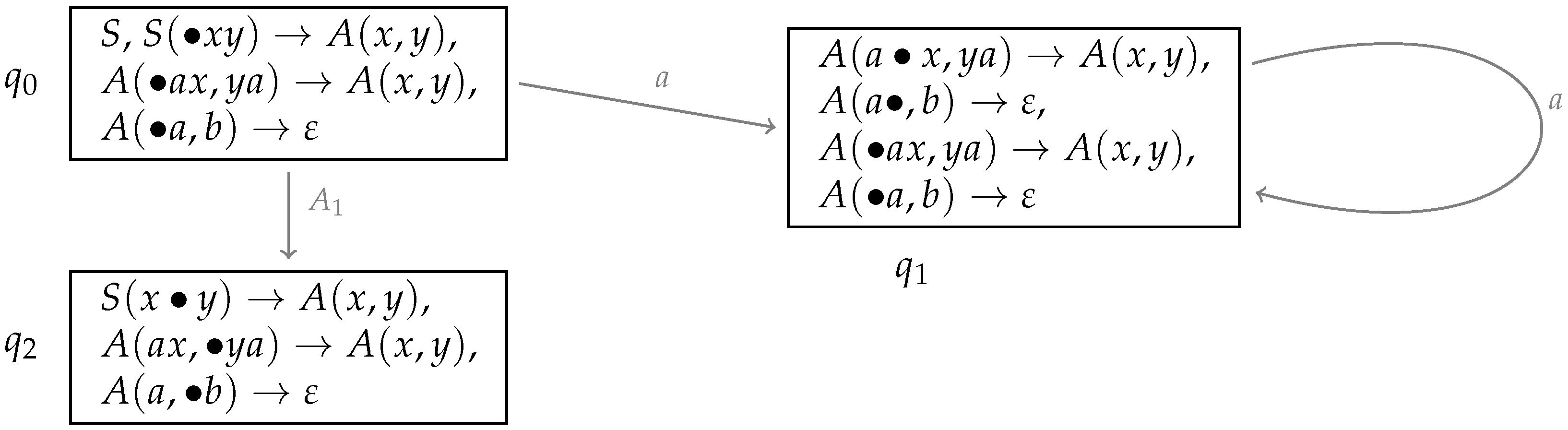
4.4. An Example with Crossing Dependencies

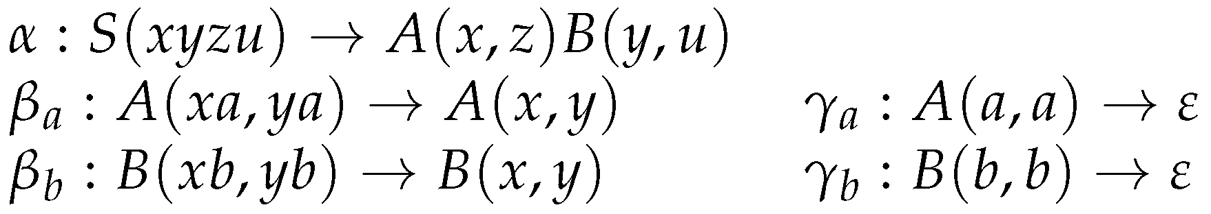
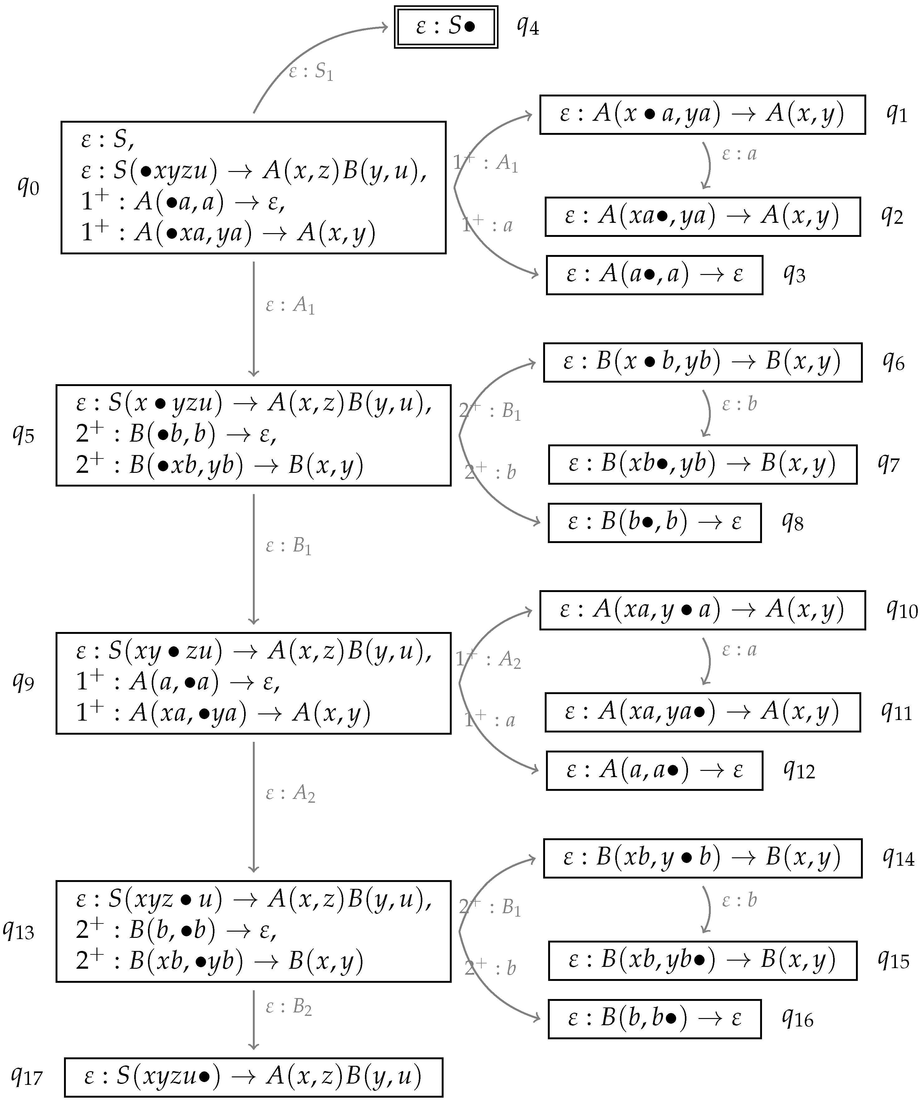
The running example we have considered so far generates only a context-free language. It was chosen for its simplicity and for the fact that it has a non-terminal with a fan-out $>1$ and a left recursion in one of the components, which requires the use of regular expressions. Let us now consider the LCFRS in Figure 16, an LCFRS for a language that is not context-free with a cross-serial dependency structure. We have again left recursions, this time in all components of the rules ${\beta }_a$ and ${\beta }_b$. And the rank of the grammar is 2, not 1 as in the running example we have considered so far. This gives us more interesting derivation trees.

The LR automaton for this grammar is given in Figure 17. Since we have a left recursion in both components of the β rules, the predict and resume closures of the items that start the traversal of these components contain each an infinite number of addresses in the derivation tree, encoded in a regular expression ($1^{+}$ or $2^{+}$). This automaton leads then to the parse table in Figure 18. As can be seen, the grammar does not allow for a deterministic parsing since, when being in $q_0$ for instance and having completed the first component of an A, this can lead to $q_1$ or $q_5$, consequently there are several entries in the corresponding goto-field.

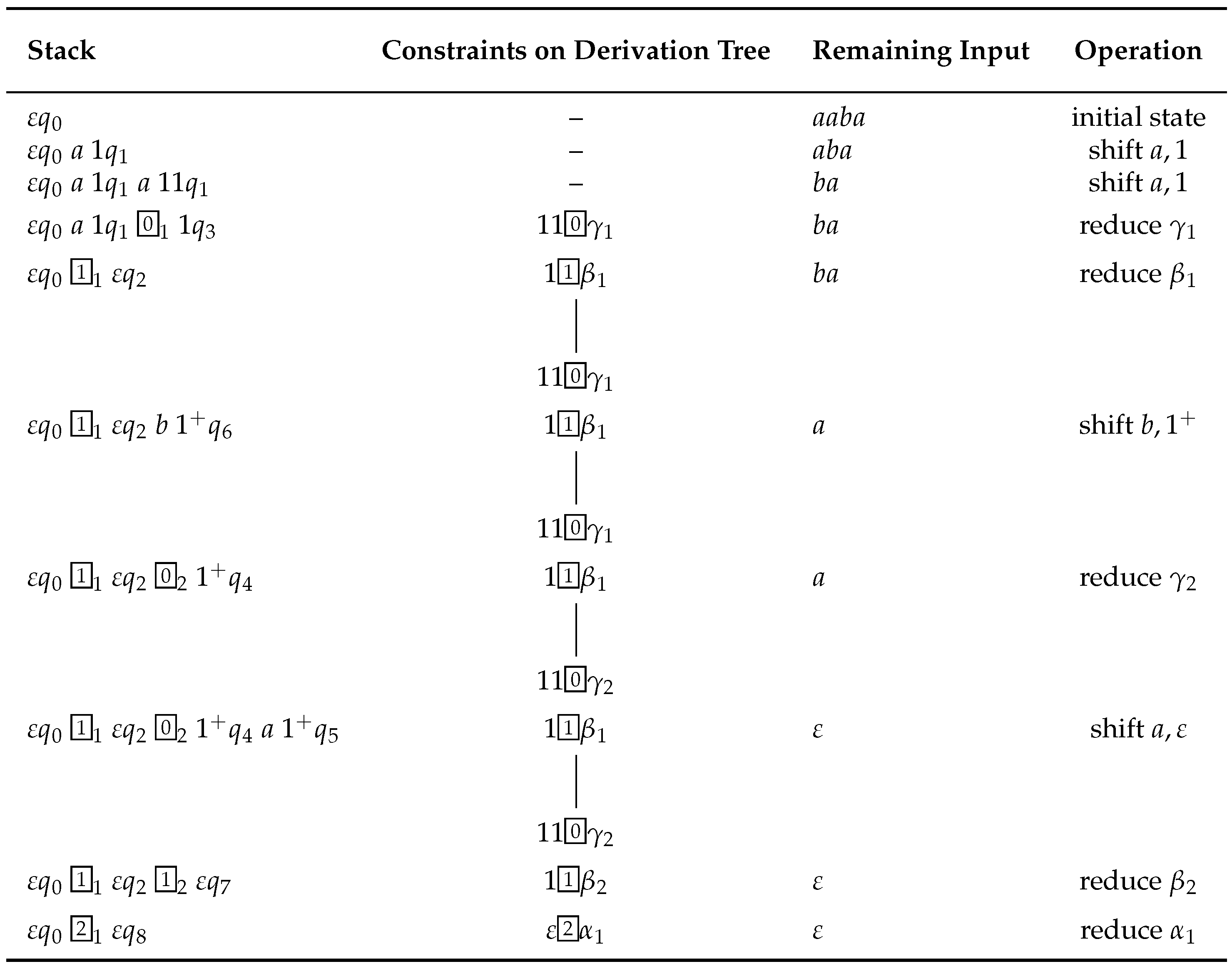
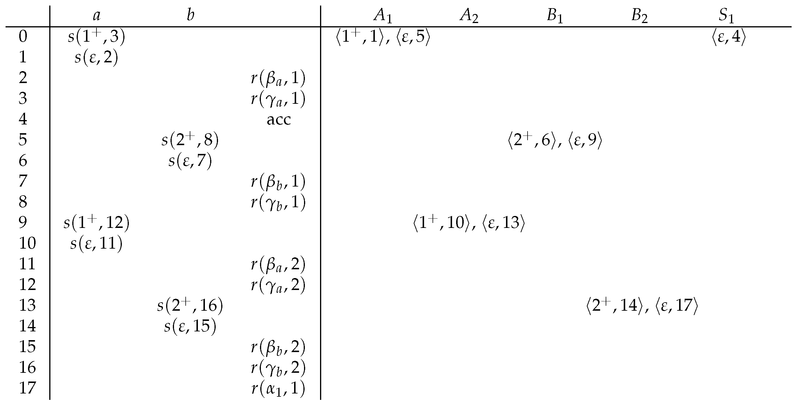
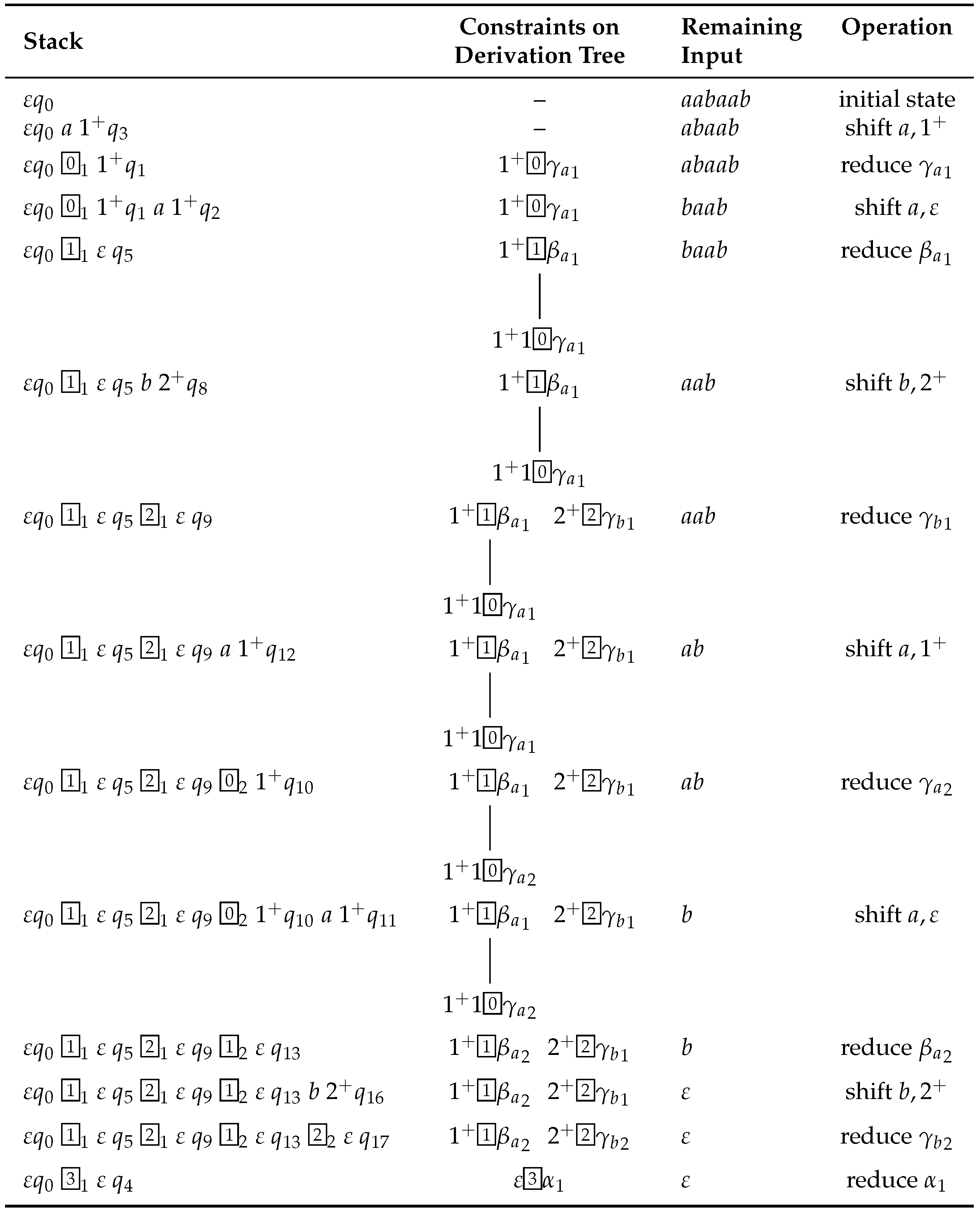
Figure 19 gives a sample parse (only successful configurations) for the input $aabaab$. When reducing the components of the A yields (nodes $\boxed{0}$ and $\boxed{1}$) and of the components of the B yields ($\boxed{2}$), we do not know the exact address of these elements in the derivation tree. Only in the last reduce step, it becomes clear that the $\boxed{1}$ and $\boxed{2}$ nodes are immediate daughters of the root of the derivation tree, and their addresses are resolved to 1 and 2 respectively.

As mentioned, this grammar does not allow for a deterministic parsing. With one additional lookahead, the grammar would become deterministic (the ε-possibility is to be taken when being at the end of one of the $a^n$ or $b^m$ substrings of the input).

4.5. Deterministic Parsing

As mentioned, with one lookahead, LR parsing of the LCFRS in the previous example would become deterministic.

In general, when doing natural language processing, the grammars will always be ambiguous and a deterministic parsing is not possible. Instead, some way to share structure in the style of generalized LR [29] parsing has to be found. In other applications, however, we might have LCFRSs that allow for a deterministic parsing, similar to LR(k) parsing as in [27].

Non-determinism with LCFRS can arise not only from shift-reduce or reduce-reduce conflicts as in CFGs but also from a conflict between different $\mathit{goto}$ transitions that have the same component non-terminal but different node addresses (see the multiple entries in the $\mathit{goto}$ table of our example). We therefore need lookaheads not only for reduce (and, if $k>1$, shift) but also for the $\mathit{goto}$ entries.

We now define, similar to the CFG case [27], sets of $\mathit{First}$ symbols for dotted productions, which contain all terminals that are reachable as first element of the yield, starting from the dotted production. For every ${\gamma }_{i,j}$, let us define $\mathit{First}(\gamma ,i,j)$ as follows. (Remember that $\mathit{lhs}(\gamma ,i,j)$ gives the jth symbol of the ith component in the lefthand side of γ, i.e., the element following the dot.)

• $\epsilon \in \mathit{First}(\gamma ,i,j)$ if $\mathit{lhs}(\gamma ,i,j)$ is not defined (i.e, the dot is at the end of the ith component);
• $a\in \mathit{First}(\gamma ,i,j)$ if $\mathit{lhs}(\gamma ,i,j)=a$ (i.e., the dot precedes a);
• $a\in \mathit{First}(\gamma ,i,j)$ if $\mathit{lhs}(\gamma ,i,j)=x\in V$, x is the lth component in a righthand side element of γ with non-terminal B, and there is a ${\gamma }_B\in P$ with $\mathit{lhs}\left({\gamma }_B\right)=B$ such that $a\in \mathit{First}({\gamma }_B,l,0)$.
• Nothing else is in $\mathit{First}(\gamma ,i,j)$.

Besides this, we also need the notion of $\mathit{Follow}$. $\mathit{Follow}$ sets are defined for all component nonterminals $A_i$ ($A\in N,1\le i\le \mathit{dim}\left(A\right)$) of our LCFRS. They contain the terminals that can immediately follow the yield of such a component nonterminal.

• $\$\in \mathit{Follow}\left(S_1\right)$ where S is the start symbol and $\$\notin T$ is a new symbol marking the end of the input.
• For every production γ with $x\in V$ being the jth element of the ith lefthand side component (indices start with $i=0$ and $j=0$) and x being the lth element of the yield of a nonterminal B in the righthand side (also starting with $l=0$), we have $\mathit{First}\left({\gamma }_{i,j+1}\right)\subseteq \mathit{Follow}\left(B_{l+1}\right)$, provided $\mathit{First}\left({\gamma }_{i,j+1}\right)$ is defined.
• For every production γ with $\mathit{lhs}\left(\gamma \right)=A$ and with $x\in V$ being the last element of the ith lefthand side component (indices start with $i=0$) and the lth element of the yield of a nonterminal B in the righthand side (also starting with $l=0$), we have $\mathit{Follow}\left(A_{i+1}\right)\subseteq \mathit{Follow}\left(B_{l+1}\right)$.
• Nothing else is in the sets $\mathit{Follow}\left(A_i\right)$ of our component nonterminals.

For $LR\left(1\right)$ parsing, i.e., LR parsing with 1 lookahead, we replace the items in our states with triples consisting of the adress (regular expression), the dotted production ${\gamma }_{i,j}$ and the possible next terminal symbols. To this end, we define sets $\mathit{Next}(\gamma ,i,j)$ that are the $\mathit{First}$ sets for dots that are not at the end of components and otherwise the $\mathit{Follow}$-sets of the component non-terminal:

$\mathit{Next}(\gamma ,i,j)=\mathit{First}(\gamma ,i,j)$ if ${\gamma }_{i,j+1}$ exists and $\mathit{Next}(\gamma ,i,j)=\mathit{Follow}\left(\mathit{lhs}{\left(\gamma \right)}_{i+1}\right)$ otherwise.

A simple way to extend our automaton to $LR\left(1\right)$ is by extending the items in the states as follows: Every item with dotted production ${\gamma }_{i,j}$ is equipped with the lookahead set $\mathit{Next}(\gamma ,i,j)$. Furthermore, transitions are also labeled with triples where the new third element that is added is the terminal in case of a shift transition and, in case of a transition that moves the dot over a non-terminal, the $\mathit{Next}$ set of the result of moving the dot according to the transition.

Consider the sample automaton in Figure 17. $q_0$ has two outgoing $A_1$ edges with different addresses. One (derivation tree node address ε) arises from moving the dot over the variable x in $S(•xyzu)\to A(x,z)B(y,u)$. We have $\mathit{Next}\left(S\right(x•yzu)\to A(x,z\left)B\right(y,u\left)\right)=\mathit{First}\left(B\right(•b,b)\to \epsilon )\cup \mathit{First}\left(B\right(•xb,yb)\to B(x,y\left)\right)=\left\{b\right\}$, therefore this transition would be relabeled $\epsilon :A_1:\left\{b\right\}$. The other transition (address $1^{+}$) leads to $A(x•a,ya)\to A(x,y)$, the $\mathit{First}$ set is $\left\{a\right\}$ and therefore this transition would be relabeled $1^{+}:A_1:\left\{a\right\}$.

Consequently, the $\mathit{goto}$ part of the parse table, that would now have entries for every combination of component non-terminal and lookahead symbol, would have at most one entry per field. Hence, LR(1) parsing of our sample grammar is deterministic.

Concerning the reduce steps in the parse table, we would also have a lookahead. Here we can use the elements from the $\mathit{Follow}$ set of the reduced components as lookaheads. The $r({\beta }_a,1)$ reduce entry for state $q_2$ for instance would have the lookaheads from $\mathit{Follow}\left(A_1\right)=\{a,b\}$.

Instead of this simple LR technique one can also compute the lookahead sets while constructing the automaton, in the style of canonical LR parsing for CFGs. This would allow for more precise predictions of next moves.

There are LCFRSs that do not allow for a deterministic $LR$ parsing, no matter how long the length k of the lookahead strings (the non-deterministic CFGs, which are 1-LCFRSs are such grammars). But a precise characterization of the class of deterministic LCFRSs and an investigation of whether, for every $LR\left(k\right)$ LCFRS, we can find a weakly equivalent $LR\left(0\right)$ LCFRS (as is the case for CFG), is left for further research.

4.6. Soundness and Completeness of the LR Algorithm

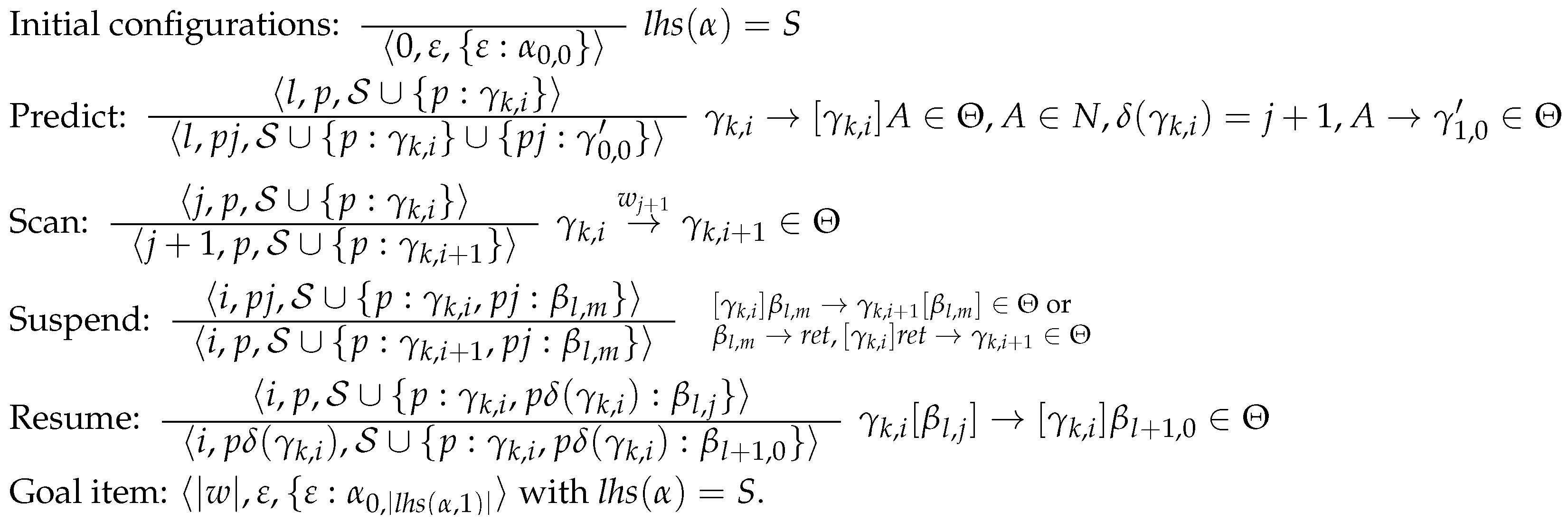
In order to show soundness and completeness of the LR algorithm, we will relate it to the LCFRS-TA for the same grammar. We will slightly modify the deduction rules for TA by assuming that (1) call and predict steps are combined and the initial configuration is omitted, i.e., we start with the result of the first predict steps; (2) we omit the publish steps; and (3) we don’t delete threads of finished rules. The modified rules are given Figure 20. Concerning the LR automaton, we replace the regular expressions in our parsing configurations with concrete addresses. In principal we can then have infinitely many configurations in cases of left recursions (just like in the TA case), i.e., in cases where a shift or goto transition comes with a regular expression denoting an infinite language. Furthermore, we do not delete daughters of completed rules in the constraint set either, i.e., we assume that the rule 2(b) in Definition 11 concerning the application of $f_{⊲}$ to the constraint set does not apply. Clearly, this does not change the languages recognized by these automata, it just increases the set of possible configurations. Since we use no longer regular expressions but single addresses, the deduction rules of the LR parser get simpler. Immediate dominance constraints are no longer needed since they follow from the addresses. The relevant deduction rules are given in Figure 21.

Figure 22 shows the correspondence between TA configurations and LR configurations for our sample derivation of $aaba$.

We now define a function $f_{\mathit{TA}}$ that gives for every LR configuration the set of corresponding TA configurations. The idea is the following: An LR configuration describes a path in our LR automaton. This path yields several possible thread contents.

Before giving the formal definition, let us consider two examples from Figure 22 for illustration. Take as a first example the LR configuration $\langle \epsilon q_{0}a1q_{1}a11q_1,\varnothing ,2\rangle$. The corresponding path in our automaton is

$$\epsilon :q_0\boxed{\begin{array}{l}\epsilon :S,\epsilon :{\alpha }_{0,0},\\ 1:{\beta }_{0,0},1:{\gamma }_{0,0}\end{array}}\stackrel{1:a}{\to }\stackrel{1:q_1}{\boxed{\begin{array}{c}\epsilon :{\beta }_{0,1},\epsilon :{\gamma }_{0,1}\\ 1:{\beta }_{0,0},1:{\gamma }_{0,0}\end{array}}}\stackrel{1:a}{\to }\stackrel{11:q_1}{\boxed{\begin{array}{c}\epsilon :{\beta }_{0,1},\epsilon :{\gamma }_{0,1}\\ 1:{\beta }_{0,0},1:{\gamma }_{0,0}\end{array}}}$$

Each thread store in the corresponding TA configuration corresponds to a possible path through these states.

• For every ε-element in the last state of this path (here $\epsilon :{\beta }_{0,1}$ or $\epsilon :{\gamma }_{0,1}$), we compute the TA configurations $\langle 2,11,{\mathcal{S}}_{\beta }\rangle$ and $\langle 2,11,{\mathcal{S}}_{\gamma }\rangle$ respectively for these elements:
  Let us consider first the case of ${\mathcal{S}}_{\beta }$. We first define a set ${\mathcal{S}}_{\beta }^{\prime }$, starting with ${\mathcal{S}}_{\beta }^{\prime }=\{11:{\beta }_{0,1}\}$:

  -

  Since $11:{\beta }_{0,1}$ was obtained via the a-transition, from $1:{\beta }_{0,0}$ in $1:q_1$, we add $11:{\beta }_{0,0}$ to ${\mathcal{S}}_{\beta }^{\prime }$.

  -

  $11:{\beta }_{0,0}$ in turn is in the second state on the path since we obtained it via prediction from $1:{\beta }_{0,1}$, which is added to ${\mathcal{S}}_{\beta }^{\prime }$ as well.

  -

  Again, $1:{\beta }_{0,1}$ arose out of a shift of a from $1:{\beta }_{0,0}$, which is added as well and then, because of predict in $q_0$, we add $ϵ:{\alpha }_{0,0}$. This gives ${\mathcal{S}}_{\beta }^{\prime }=\{11:{\beta }_{0,1},11:{\beta }_{0,0},1:{\beta }_{0,1},1:{\beta }_{0,0},ϵ:{\alpha }_{0,0}\}$.

  -

  We then remove all items where there is an item with the same address and rule in the set but with a lefthand side index that is more advanced. This yields ${\mathcal{S}}_{\beta }^{\prime }=\{11:{\beta }_{0,1},1:{\beta }_{0,1},ϵ:{\alpha }_{0,0}\}$, which is the thread set ${\mathcal{S}}_{\beta }$ we were looking for.

  -

  In a similar way, for the γ case, we obtain ${\mathcal{S}}_{\gamma }=\{11:{\gamma }_{0,1},1:{\beta }_{0,1},ϵ:{\alpha }_{0,0}\}$

• In addition, we add all configurations that we can reach from the ones constructed so far via predict or resume. These are reflected in corresponding items in the last state of our path. In our sample case, $1:{\beta }_{0,0}$ and $1:{\gamma }_{0,0}$ are both elements of the last state and arose directly out of $ϵ:{\beta }_{0,1}$ via predict. Therefore, we add these to the thread store with $11:{\beta }_{0,1}$ being the active thread, which leads to $\langle 2,111,\{\epsilon :{\alpha }_{0,0},1:{\beta }_{0,1},11:{\beta }_{0,1},111:{\beta }_{0,0}\}\rangle$ and $\langle 2,111,\{\epsilon :{\alpha }_{0,0},1:{\beta }_{0,1},11:{\beta }_{0,1},111:{\gamma }_{0,0}\}\rangle$.
• These are all configurations in $f_{\mathit{TA}}\left(\langle \epsilon q_{0}a1q_{1}a11q_1,\varnothing ,2\rangle \right)$.

Now consider as a second example $\langle \epsilon :q_0{\boxed{1}}_1\epsilon :q_{2}b11:q_6,\{11\boxed{0}{\gamma }_1,1\boxed{1}{\beta }_1\},3\rangle$, corresponding to the following path:

$$\epsilon :q_0 \boxed{\begin{array}{l}\epsilon :S,\epsilon :{\alpha }_{0,0}\\ 1:{\beta }_{0,0},1:{\gamma }_{0,0}\end{array}}\stackrel{\epsilon :A_1}{\to }\stackrel{\epsilon :q_2}{\boxed{\begin{array}{l}\epsilon :{\alpha }_{0,1}\\ 1^{+}:{\beta }_{1,0},1^{+}:{\gamma }_{1,0}\end{array}}}\stackrel{1^{+}:b}{\to }\stackrel{1^{+}:q_6}{\boxed{\epsilon :{\gamma }_{1,1}}}$$

Again, we have to go back from the ε-element in the last state in order to construct the thread store. The last element gives us $11:{\gamma }_{1,1}$.

Consequently, the configuration is $\langle 3,11,\mathcal{S}\rangle$ and we construct $\mathcal{S}$ starting with ${\mathcal{S}}^{\prime }=\{11:{\gamma }_{1,1}\}$. Following the shift transition back adds $11:{\gamma }_{1,0}$ to ${\mathcal{S}}^{\prime }$. $11:{\gamma }_{1,0}$, in turn, arose from a resume applied to $1:{\beta }_{1,0}$, which is therefore added as well. $1:{\beta }_{1,0}$ was predicted from $\epsilon :{\alpha }_{0,1}$, which is added as well. Now we follow the $A_1$-transition backwards and therefore add $\epsilon :{\alpha }_{0,0}$. Finally, since for a specific address and rule, we keep only the most advanced position, we obtain $\langle 3,11,\{\epsilon :{\alpha }_{0,1},1:{\beta }_{1,0},11:{\gamma }_{1,1}\}\rangle$.

In order to define the corresponding TA-sets, we annotate the LR automaton with pointers that show for each element c in any of the states, which other element $c^{\prime }$ has lead to c, either because of moving the dot over a terminal or a component variable or because of a predict/resume closure operation. In the latter case, the pointer is labeled with the daughter index of the predict/resume operation. For this annotation, we assume that instead of pairs $r:c$ of regular expression and comutation point, we use onyl pairs $p:c$ of address and computation point. This means of course, that we have potentially infinite states and potentially infinite predecessor paths through a state and from one state to another.

Definition 12 (Predecessor Annotation). 

Let M be an LR-automaton with state set Q constructed from an LCFRS G. $\mathcal{Q}=\{\langle x,q\rangle |q\in Q,x\in q\}$.

We define the predecessor annotation of M as a labeled relation $\mathit{Predec}\subset \mathcal{Q}\times \mathcal{Q}\times ({\{1,\cdots ,\mathit{rank}\left(G\right)\}}^{*}\cup \{-\})$ such that for every $q\in Q$ and every $p:c\in q$:

• If there is a $p^{\prime }:c^{\prime }\in q$ such that $p=p^{\prime }i$ and $pi:c$ can be deduced from $p:c^{\prime }$ by the predict/resume rule from Definition 7, $\langle \langle p:c,q\rangle ,\langle p^{\prime }:c^{\prime },q\rangle ,i\rangle \in \mathit{Predec}$.
• If $p=\epsilon$ and there is a $q^{\prime }\in Q$ and a $p^{\prime }:c^{\prime }\in q^{\prime }$ such that $\epsilon :c\in \mathit{read}(\{p^{\prime }:c^{\prime }\},x,p^{\prime })$ for some $x\in T\cup \left\{A_i\right|A\in N,1\le i\le \mathit{dim}\left(A\right)\}$, then $\langle \langle p:c,q\rangle ,\langle p^{\prime }:c^{\prime },q^{\prime }\rangle ,-\rangle \in \mathit{Predec}$.

Nothing else is in $\mathit{Predec}$.

Now we can define the set of possible TA stores for a given LR-configuration.

For every set of constraints C, we define $\mathit{Nodes}\left(C\right)$ as the set of pointers in C. Furthermore, for every pointer $\boxed{i}\in \mathit{Nodes}(C)$, we define $\mathit{addr}(\boxed{i},C)$ as the address associated with $\boxed{i}$, and $\mathit{label}(\boxed{i},C)$ as its label ${\beta }_j$.

For a given LR configuration, we compute the corresponding TA configurations via deduction rules. The items in these rules have the form $[\mathcal{S},\langle \mathrm{\Gamma },C\rangle ,i,p,p_2:c]$ with $\mathcal{S}$ a thread store, $\langle \mathrm{\Gamma },C\rangle$ a LR configuration, i the index in the input, p an address and $p_2:c$ an element of the topmost state in Γ. We start with an empty thread store and our LR configuration. The deduction rules then either move backwards inside the topmost Γ state or remove elements from Γ while adding corresponding threads to the thread store. In the end, we will have an empty stack Γ and then, the thread store $\mathcal{S}$ together with the index i and the address p of the current thread gives us one of the TA configurations corresponding to the LR configuration we started with. p stays constant throughout the entire computation. $p_1$ represents the address of the daughter that has lead to moving into the current state.

Definition 13. 

Let G be an LCFRS, $M_G$ its LR automaton. For every input $w\in T^{*}$ and every configuration $\langle \mathrm{\Gamma },C,i\rangle$ that can be deduced via $M_G$ for the input w, we define $f_{\mathit{TA}}\left(\langle \mathrm{\Gamma },C,i\rangle \right)=\left\{\langle i,p,\mathcal{S}\rangle \right|[\mathcal{S},\langle \epsilon ,\varnothing \rangle ,i,p,-,-]$ can be deduced from $[\varnothing ,\mathrm{\Gamma },C,i,-,-,-]$ via the following deduction rules}.

• Current thread: $\frac{[\varnothing ,\langle \mathrm{\Gamma }{p}_{1}q,C\rangle ,i,-,-]}{[\{p_1{p}_2:c\},\langle \mathrm{\Gamma }{p}_{1}q,C\rangle ,i,p_1{p}_2,p_2:c]}{p}_2:c\in q$
• Predict/resume backwards:$\frac{[\mathcal{S},\langle \mathrm{\Gamma }{p}_{1}q,C\rangle ,i,p,p_{2}j:c]}{[\mathcal{S}\cup \{p_1{p}_2:c^{\prime }\},\langle \mathrm{\Gamma }{p}_{1}q,C\rangle ,i,p,p_2:c^{\prime }]}\begin{array}{c}\langle \langle p_{2}j:c,q\rangle ,\langle p_2:c^{\prime },q\rangle ,j\rangle \hfill \\ \in \mathit{Predec}\hfill \end{array}$
• Shift backwards:$\frac{[\mathcal{S},\langle \mathrm{\Gamma }{p}_1{q}^{\prime }a{p}_1{p}_{2}q,C\rangle ,i,p,\epsilon :c]}{[\mathcal{S},\langle \mathrm{\Gamma }{p}_1{q}^{\prime },C\rangle ,i,p,p_2:c^{\prime }]}\begin{array}{c}a\in T\hfill \\ and\langle \langle \epsilon :c,q\rangle ,\langle p_2:c^{\prime },q^{\prime }\rangle ,-\rangle \in \mathit{Predec}\hfill \end{array}$
• Shift non-terminal backwards:$\frac{[\mathcal{S},\langle \mathrm{\Gamma }{p}_1{q}^{\prime }{\boxed{k}}_j{p}_1{p}_{2}q,C\rangle ,i,p,\epsilon :c]}{[\mathcal{S},\langle \mathrm{\Gamma }{p}_1{q}^{\prime },C\rangle ,i,p,p_2:c^{\prime }]}\begin{array}{c}\exists nsuchthat{p}_1{p}_{2}n=\mathit{addr}(\boxed{k},C)and\hfill \\ \langle \langle \epsilon :c,q\rangle ,\langle p_2:c^{\prime },q^{\prime }\rangle ,-\rangle \in \mathit{Predec}\hfill \end{array}$
• Empty stack:$\frac{[\mathcal{S},\langle \epsilon q_0,C\rangle ,i,p,\epsilon :c]}{[\mathcal{S},\langle \epsilon ,C\rangle ,i,p,-]}$
• Add completed components:$\frac{[\mathcal{S},\langle \epsilon ,C\rangle ,i,p,-]}{[\mathcal{S}\cup \{p^{\prime }:{\beta }_{i-1,\left|\mathit{lhs}\right(\beta ,i\left)\right|}\},\langle \epsilon ,C\rangle ,i,p,-]}\begin{array}{c}{p}^{\prime }\boxed{k}{\beta }_i\in C,\hfill \\ p^{\prime }doesnotoccurin\mathcal{S}\hfill \end{array}$

Current thread picks one element $p_2:c$ from the topmost state q in Γ as the starting element. The address of the corresponding thread is a concatenation of the address $p_1$ preceding q on the stack and the address $p_2$ of the chosen state element. Predict/resume backwards applies whenever the address of the current state element is not ε, we then follow the $\mathit{Predec}$ link and add a corresponding new thread to our thread store. Shift backwards follows a $\mathit{Predec}$ link that corresonds to a reversed edge in the automaton labeled with a terminal. In this case, we do not change the thread store since we already have a thread for the rule application in question with a more advanced index. We only remove the shifted terminal and state from the LR stack and we split the address of the state and the element within it according to the $\mathit{Predec}$ link. Shift non-terminal backwards is a similar move following a $\mathit{Predec}$ link that corresonds to a reversed edge in the automaton labeled with a component non-terminal. These four rules serve to reduce the LR stack while constructing threads out of it. This process terminates with a single application of Empty stack. Once the stack is empty, we have to take care of the components described in C. For all of these, if no corresponding thread exists, wee add it by applying Add completed component.

Lemma 14. 

Let $G=(N,T,V,P,S)$ be a LCFRS of rank m. Let $\langle N^{\prime },T,S,\mathit{ret},\delta ,\Theta \rangle$ be the LCFRS-TA of G, and let M be the LR-automaton constructed for G with $\langle \mathit{action},\mathit{goto}\rangle$ being the LR parse table one can read off M.

For every input word $w\in T^{*}$, with ${\mathcal{C}}_{TA}$ being the set of TA configurations, ${\mathcal{C}}_{LR}$ the set of LR configurations arising from parsing w with the TA or the LR parser:

$${\mathcal{C}}_{TA}=\bigcup _{c_{LR}\in {\mathcal{C}}_{LR}}{f}_{\mathit{TA}}\left(c_{LR}\right)$$

Proof. 

Proof by induction over the deduction rules of the TA automaton and the LR parser:

• Initial configurations: $c_0=\langle \epsilon q_0,\varnothing ,0\rangle \in {\mathcal{C}}_{LR}$ can be added as initial configuration in the LR parser iff $\langle 0,\epsilon ,\{\epsilon :{\alpha }_{0,0}\}\rangle$ for every $\alpha \in P$ with $\mathit{lhs}\left(\alpha \right)=S$ are initial configurations in the TA and, furthermore, for any configuration one can obtain from one of these initial TA configurations via applications of Predict it holds that there is a corresponding element in $q_0$. Conversely, except for $\langle \epsilon :S\rangle \in q_0$, for every element in $q_0$, there is a corresponding configuration in the TA containing this element and all its predecessors as threads.
  Predict in the TA starting from any of the $\langle 0,\epsilon ,\{\epsilon :{\alpha }_{0,0}\}\rangle$:
  $\frac{\langle 0,p,\mathcal{S}\cup \{p:{\gamma }_{0,0}\}\rangle }{\langle 0,pj,\mathcal{S}\cup \{p:{\gamma }_{0,0}\}\cup \{pj:{\gamma }_{0,0}^{\prime }\}\rangle }\begin{array}{c}{\gamma }_{0,0}\to \left[{\gamma }_{0,0}\right]A\in \Theta ,A\in N,\delta \left({\gamma }_{0,0}\right)=j+1,\hfill \\ A\to {\gamma }_{1,0}^{\prime }\in \Theta ,i.e.,A=\mathit{lhs}\left({\gamma }^{\prime }\right)\hfill \end{array}$
  Elements in $q_0$ are obtained by

  -

  Initial predict: $\frac{\epsilon :S}{\epsilon :{\alpha }_{0,0}}\begin{array}{c}\mathit{lhs}\left(\alpha \right)=S\hfill \end{array}$

  -

  Predict closure on $q_0$ in the LR automaton: $\frac{p:{\gamma }_{0,0}}{pj:{\gamma }_{0,0}^{\prime }}\begin{array}{c}\mathit{lhs}(\gamma ,0,0)=\mathit{rhs}(\gamma ,j-1,0),\hfill \\ \mathit{rhs}(\gamma ,j)=\mathit{lhs}\left({\gamma }^{\prime }\right)\hfill \end{array}$

  with a $\mathit{Predec}$ link labeled j from the consequent item to the antecedent item.

  Consequently, we obtain that the set of TA configurations we get by using only the initial rule and Predict is exactly $f_{TA}\left(c_0\right)$, i.e., the union of all $f_{TA}\left(c\right)$ for LR configurations we can obtain by the initial rule.
• Scan and Shift: We now assume that we have sets ${\mathcal{C}}_{TA}$ of TA configurations and ${\mathcal{C}}_{LR}$ of LR configurations such that ${\mathcal{C}}_{TA}={\bigcup }_{c_{LR}\in {\mathcal{C}}_{LR}}{f}_{\mathit{TA}}\left(c_{LR}\right)$.
  To show: For any pair $c_{LR},f_{\mathit{TA}}\left(c_{LR}\right)$ contained in the two sets and for any terminal a and any address p: $c_{TA,1},\cdots ,c_{TA,k}$ are all the configurations in $f_{\mathit{TA}}\left(c_{LR}\right)$ with current thread address p that allow for an application of Scan with a, the new configurations being $c_{TA,1}^{\prime },\cdots ,c_{TA,k}^{\prime }$ iff $c_{LR}$ allows to derive a new configuration $c_{LR}^{\prime }$ via an application of Shift with the terminal a and address p, such that the following holds: $f_{\mathit{TA}}\left(c_{LR}^{\prime }\right)={\bigcup }_{i=1}^k\overline{c_{TA,i}^{\prime }}$ where $\overline{c_{TA}^{\prime }}$ is the closure of $\left\{c_{TA}^{\prime }\right\}$ under applications of Predict and Resume.
  Let us repeat the operations Scan and Shift:
  Scan in the TA: $\frac{\langle j,p,\mathcal{S}\cup \{p:{\gamma }_{k,i}\}\rangle }{\langle j+1,p,\mathcal{S}\cup \{p:{\gamma }_{k,i+1}\}\rangle }\begin{array}{c}{\gamma }_{k,i}\stackrel{w_{j+1}}{\to }{\gamma }_{k,i+1}\in \Theta \hfill \end{array}$
  Shift in the LR automaton: $\frac{\langle \mathrm{\Gamma }{p}_{1}q,C,j\rangle }{\langle \mathrm{\Gamma }{p}_{1}q{w}_{j+1}{p}_1{p}_2{q}^{\prime },C,j+1\rangle }\begin{array}{c}\mathit{action}(q,w_{j+1})\hfill \\ =s(r,q^{\prime }),p_2\in L\left(r\right)\hfill \end{array}$
  Let $c_{TA,i}=\langle j,p,\mathcal{S}\cup \{p:{\gamma }_{m_i,n_i}^i\}\rangle$ for $1\le i\le k$. According to our induction assumption, $c_{LR}$ has a form $\langle \mathrm{\Gamma }{p}_{1}q,C,j\rangle$ such that there exist a $p_2:{\gamma }_{m_i,n_i}^i\in q$ with $p=p_1{p}_2$ for all $1\le i\le k$. Furthermore, the dot in ${\gamma }_{m_i,n_i}^i$ precedes a terminal $a=w_{j+1}$, we consequently can perform scans on $c_{TA,1},\cdots ,c_{TA,k}$ and there is a shift transition $\mathit{action}(q,a)=s(r,q^{\prime }),p_2\in L\left(r\right)$. Consequently, we can obtain new TA configurations $c_{TA,i}^{\prime }=\langle j+1,p,\mathcal{S}\cup \{p:{\gamma }_{m_i,n_i+1}^i\}\rangle$ and a new LR configuration $\langle \mathrm{\Gamma }{p}_{1}q{w}_{j+1}{p}_1{p}_2{q}^{\prime },C,j+1\rangle$ in the LR automaton.
  According to the LR automaton construction, $\overline{\{\epsilon :{\gamma }_{m_1,n_1+1}^1,\cdots ,\epsilon :{\gamma }_{m_k,n_k+1}^k\}}=q^{\prime }$ with $\epsilon :{\gamma }_{m_i,n_i+1}^i$ having a predecessor link pointing to $p_2:{\gamma }_{m_i,n_i}^i$ in q. Further elements in $q^{\prime }$ are obtained by predict and resume and are linked to the elements with address ε by a predecessor chain. The same predict and resume operations can be applied to the corresponding TA configurations $c_{TA,1}^{\prime },\cdots ,c_{TA,k}^{\prime }$ as well. Therefore our induction assumption holds.
• Suspend and Reduce: We assume again that we have sets ${\mathcal{C}}_{TA}$ of TA configurations and ${\mathcal{C}}_{LR}$ of LR configurations such that ${\mathcal{C}}_{TA}={\bigcup }_{c_{LR}\in {\mathcal{C}}_{LR}}{f}_{\mathit{TA}}\left(c_{LR}\right)$.
  To show: For any pair $c_{LR},f_{\mathit{TA}}\left(c_{LR}\right)$ contained in the two sets: there is a $c_{TA}\in f_{\mathit{TA}}\left(c_{LR}\right)$ that allows to derive a new configuration $c_{TA}^{\prime }$ via an application of suspend iff $c_{LR}$ allows to derive a new configuration $c_{LR}^{\prime }$ via an application of reduce 1/2 such that $f_{\mathit{TA}}\left(c_{LR}^{\prime }\right)=\overline{c_{TA}^{\prime }}$.
  Let $c_{TA}=\langle i,pj,\mathcal{S}\cup \{p:{\gamma }_{k,n},pj:{\beta }_{l,m}\}\rangle$ such that a suspend can be applied resulting in $\langle i,p,\mathcal{S}\cup \{p:{\gamma }_{k,n+1},pj:{\beta }_{l,m}\}\rangle$. According to our induction assumption, $c_{LR}$ has a form $\langle \mathrm{\Gamma }pjq,C,i\rangle$ such that there exists a $\epsilon :{\beta }_{l,m}\in q$ (without loss of generality, we assume our grammars to be ε-free. Consequently, computation points with the dot at the end of a component cannot arise from predict or resume operations and therefore always have address ε). Furthermore, since in ${\beta }_{l,m}$, the dot is at the end of the $(l+1)$th component, we have $r(\beta ,l+1)\in \mathit{action}(q,-)$.
  Let us remind the suspend and reduce operations:
  TA Suspend: $\frac{\langle i,pj,\mathcal{S}\cup \{p:{\gamma }_{k,n},pj:{\beta }_{l,m}\}\rangle }{\langle i,p,\mathcal{S}\cup \{p:{\gamma }_{k,n+1},pj:{\beta }_{l,m}\}\rangle }\begin{array}{c}\left[{\gamma }_{k,i}\right]{\beta }_{l,m}\to {\gamma }_{k,n+1}\left[{\beta }_{l,m}\right]\in \Theta or\hfill \\ {\beta }_{l,m}\to \mathit{ret},\left[{\gamma }_{k,n}\right]\mathit{ret}\to {\gamma }_{k,n+1}\in \Theta \hfill \end{array}$
  LR Reduce 1: $\frac{\langle \mathrm{\Gamma }{p}_k{q}_k{X}_k\cdots p_1{q}_1{X}_{1}pjq,C,i\rangle }{\langle \mathrm{\Gamma }{p}_k{q}_k{\boxed{l}}_1{p}_k{p}^{\prime }{q}^{\prime },C\cup \left\{pj\boxed{l}{\beta }_1\right\},i\rangle }\begin{array}{c}r(\beta ,1)\in \mathit{action}(q,-),k=\left|\mathit{lhs}\right(\gamma ,0\left)\right|,\hfill \\ \mathit{goto}(q_k,\mathit{lhs}{\left(\gamma \right)}_1)=\langle r,q^{\prime }\rangle ,p^{\prime }\in L\left(r\right),\boxed{l}\notin {\mathcal{N}}_C\hfill \end{array}$
  LR Reduce 2: $\frac{\langle \mathrm{\Gamma }{p}_k{q}_k{X}_k\cdots p_1{q}_1{X}_{1}pjq,C\cup \left\{pj\boxed{l}{\beta }_{l-1}\right\},i\rangle }{\langle \mathrm{\Gamma }{p}_k{q}_k{\boxed{l}}_l{p}_k{p}^{\prime }{q}^{\prime },C\cup \left\{pj\boxed{l}{\beta }_l\right\},i\rangle }\begin{array}{c}r(\beta ,l)\in \mathit{action}(q,-),\hfill \\ 1<l,k=\left|\mathit{lhs}\right(\beta ,l-1\left)\right|,\hfill \\ \mathit{goto}(q_k,\mathit{lhs}{\left(\beta \right)}_l)=\langle r,q^{\prime }\rangle ,p^{\prime }\in L\left(r\right)\hfill \end{array}$
  where for both reduce steps, any component pointer ${\boxed{i}}_m$ among the $X_1,\cdots ,X_k$ has an address $pjm$ for some $m\in \{1,\cdots ,|\mathit{rhs}\left(\beta \right)\left|\right\}$.
  The only difference between the two reduce steps is that in the first, a first component is found and therefore a new pointer added to C, while in the second, only the component index of an already present pointer in C is incremented.
  In our case, there must be elements $p^{\prime }:{\gamma }_{k,n},p^{\prime }j:{\beta }_{l,0}\in q_k$ such that $p_k{p}^{\prime }=p$ and $\epsilon :{\gamma }_{k,n+1}\in q^{\prime }$. This means that for the resulting LR configuration, we obtain exactly the TA thread store plus eventually additional store entries obtained from predict or resume operations.

4.7. Comparison to TAG Parsing

As mentioned in the beginning, LR parsing has also been proposed for TAG [31,41]. The LR states in this case contain dotted productions that correspond to small subtrees (a node and its daughters) in the TAG elementary trees. They are closed under moving up and down in these trees, predicting adjunctions and predicting subtrees below foot nodes. There are two different transitions labeled with non-terminal symbols in the LR automata constructed for TAG: Transitions that correspond to having finished a subtree and moving the dot over the corresponding non-terminal node and transitions that correspond to having finished the part below a foot node and moving back into the adjoined auxiliary tree. The latter transitions are labeled with the adjunction site. In the parser, when following such a transition, the adjunction site is stored on the stack of the parser. Adjunctions can be nested, consequently, we can have a list (actually a stack) of such adjunction sites that we have to go back to later. This way to keep track of where to go back to once the adjoined tree is entirely processed corresponds to the derivation node addresses we have in the thread automata and the LCFRS LR parser since both mechanisms capture the derivation structure. The difference is that with TAG, we have a simple nested structure without any interference of nested adjunctions in different places. And the contribution of auxiliary trees in the string contains only a single gap, consequently only a single element in the daughter list of a node contains such information about where to go back to when having finished the auxiliary tree. Therefore each of these chains of adjunctions can be kept track of locally on the parser stack.

Restricting our LR parser to well-nested 2-LCFRS amounts to restricting it to TAG. This restriction means that our LCFRS rules have the following form: Assume that $\gamma =A({\alpha }_0,\dots ,{\alpha }_{\mathit{dim}\left(A\right)-1})\to A_1(x_0^{\left(1\right)},\cdots ,x_{\mathit{dim}\left(A_1\right)-1}^{\left(1\right)})\cdots A_m(x_0^{\left(m\right)},\cdots ,x_{\mathit{dim}\left(A_m\right)-1}^{\left(m\right)})$ is a rule in such an LCFRS. Then we can partition the righthand side into minimal subsequences $A_1\cdots A_{i_1}$, ..., $A_{i_k}\cdots A_m$ such that a) the yields of these subsequences do not cross; b) every subsequence either (i) contains only a single non-terminal or (ii) has a first element of fan-out 2 that wraps around the yields of the other non-terminals. In this latter case, the yield of the second to last non-terminals can again be partitioned in the same way. Consider as an example a rule $A\left(x_1{x}_2{x}_3{x}_4{x}_5{x}_6{x}_7\right)\to B\left(x_1\right)C(x_2,x_6)D(x_3,x_5)E\left(x_4\right)F\left(x_7\right)$. Here, we can partition the righthand side into the daughter sequences B and $C,D,E$ and F that can be parsed one after the other without having to jump back and forth between them. Concering $C,D,E$, the C wraps around $D,E$ and, concerning this shorter sequence, D wraps around E. This means that during parsing, when processing the yield of one of these subsequences, we have to keep track of the last first component of some non-terminal that we have completed since this will be the first one for which we have to find a second component. We can push this information on a stack and have to access only the top-most element. There is no need to search through the entire partial derivation structure that has already been built in order to find a matching first component when reducing a second one. On the parse stack, it is enough to push the rule names for which we have completed a first component and still need to find a second. Pointers to the derivation structure are no longer needed. And node addresses are not needed either. Besides nestings between sisters as in this example, we can also have embedded nestings in the sense that a first comoponent is part of some other component. In this case, we have to finish the lower non-terminal before finishing the higher. In reductions of first components, we keep can keep track of embedded first components by removing them from the stack and popping them again after having added the new element. This makes sure that the second component of the most deeply embedded first component inside the rightmost first component of what we have processed so far must be completed next.

The LR automaton does not need node addresses any longer. Besides this, it looks exactly like the automata we have built so far. As an example consider the LR automaton in Figure 23.

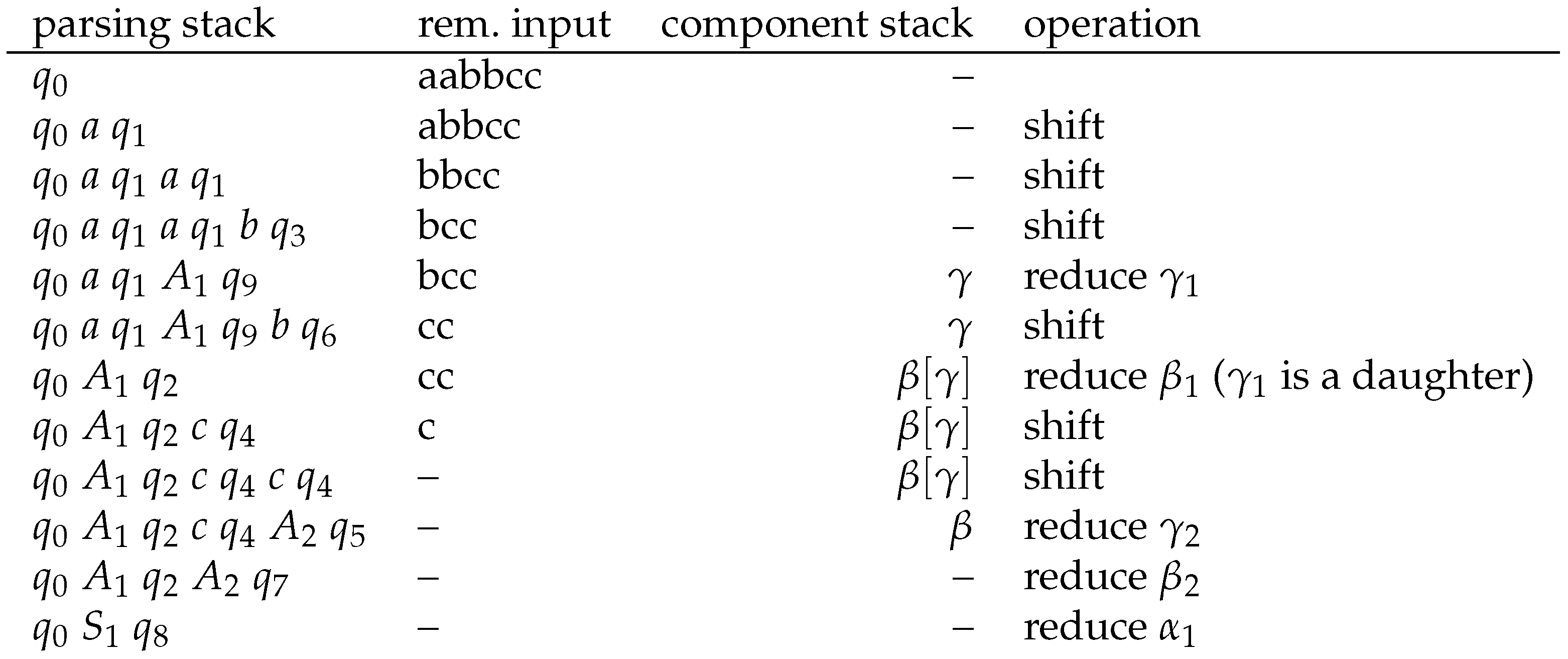
Whenever we reduce a first component of a rule with fan-out 2, we push the rule name on the component stack and any stack symbols corresponding to daughters of this component (i.e., the first component non-terminals are part of the reduced yield but not the corresponding second one) are taken from this stack and then pushed on an extra stack attached to the new rule symbol, such that the rightmost daughter is the highest element on this embedded stack. Whenever we reduce a second component, we must have the corresponding rule name as the top stack element and then we can delete it. The top is defined as follows: If the top is an element without attached stack, it is itself the top of the entire stack. If not, the top of its attached stack is the top of the entire stack structure. An example is given in Figure 24. This example involves two reduce steps with first components, the first in state $q_9$ where the rule name γ is pushed on the stack. In the second reduce step, we reduce the first component of β. This contains a non-terminal $A_1$ for which we have not seen the corresponding $A_2$ yet. Therefore, one symbol is popped from the stack (for $A_1$), and the new β is pushed with an attached stack containing the removed γ. Whenever we reduce a second component of a rule, the top-most stack element must be the name of that rule.

5. Conclusions

This paper presents the first LR style algorithm for LCFRS parsing. It extends the well-known LR parsing techniques from CFG to the case of LCFRS where a single non-terminal can span several non-adjacent strings in the input. Even though the derivation structure needs to be kept track off during parsing in order to make sure that the correct components are related to each other, the proposed algorithm constructs only a finite automaton, by capturing derivation tree addresses in regular expressions whenever left recursions occur in some component.

The resulting parsing algorithm extends previous work on incremental Earley-style LCFRS parsing and on Thread Automata, an automaton model for LCFRS that proceeds in an incremental way but that does not precompile predict and resume steps the way it is proposed for the LR construction in this paper.