Article

A Direct Search Algorithm for Global Optimization

1
Instituto de las Tecnologías Avanzadas de la Producción (ITAP), Universidad de Valladolid, Paseo del Cauce 59, 47011 Valladolid, Spain
2
Centro Tecnológico Cartif, Parque Tecnológico de Boecillo 205, 47151 Bocillo, Spain
*
Author to whom correspondence should be addressed.
Algorithms 2016, 9(2), 40; https://doi.org/10.3390/a9020040
Submission received: 19 January 2016 / Revised: 25 April 2016 / Accepted: 7 June 2016 / Published: 13 June 2016

Abstract

:
A direct search algorithm is proposed for minimizing an arbitrary real valued function. The algorithm uses a new function transformation and three simplex-based operations. The function transformation provides global exploration features, while the simplex-based operations guarantees the termination of the algorithm and provides global convergence to a stationary point if the cost function is differentiable and its gradient is Lipschitz continuous. The algorithm’s performance has been extensively tested using benchmark functions and compared to some well-known global optimization algorithms. The results of the computational study show that the algorithm combines both simplicity and efficiency and is competitive with the heuristics-based strategies presently used for global optimization.

1. Introduction

An optimization problem consists of finding an element of a given set that minimizes (or maximizes) a certain value associated with each element of the set. In this paper, we are interested in minimizing the value of a real valued function defined over the n-dimensional Euclidean space. Without loss of generality, our problem is equivalent to minimizing a real valued function over the open unit n-box ( 0 , 1 ) n R n .
Let f denote a real function defined over the open unit n-box ( 0 , 1 ) n R n , and consider the following optimization problem:
min { f ( x ) : x ( 0 , 1 ) n }
The function to be minimized f is called the cost function and the unit n-box ( 0 , 1 ) n is the search space of the problem. Our aim is to obtain a point x * ( 0 , 1 ) n , such that the cost function f attains a minimum at x * , i.e., f ( x * ) f ( x ) , x ( 0 , 1 ) n . We shall make the following assumption:
A1 
The cost function f attains its minimum at a point of the search space.
If the function f is continuously differentiable in ( 0 , 1 ) n , then:
f ( x * ) = 0 , x * ( 0 , 1 )
Many optimization methods make use of the stationarity Equation (2) to compute candidate optimizer points. These methods require the explicit knowledge of the gradient, but they do not guarantee that the point obtained is an optimizer, except for a pseudoconvex function.
We shall also make an additional assumption that will restrict our alternatives to design a procedure to compute the optimum.
A2 
The gradient of the cost function is not available for the optimization mechanism.
Consequently, only function evaluations can be used to compute the minimum.
Remark 1. 
The problem Equation (1) is equivalent to unconstrained optimization. Consider the following unconstrained optimization problem:
min { f ( ξ ) : ξ R n }
and let ξ = ξ 1 ξ 2 ξ n T be the vector of variables of the cost function. The invertible transformation:
x i = 1 1 + e - ξ i
transforms the real line into the unit interval. Consequently, we can convert an unconstrained minimization problem into an open unit n-box constrained minimization problem by transforming each of its variables. Similarly, the linear transformation:
x i = ξ i - a b - a
converts the open interval ( a , b ) into the open unit interval. Consequently, both unconstrained and arbitrary open n-box optimization problems are included in our formulation. Furthermore, under Assumption A2 and by choosing appropriate values of a and b, the global minimum of function f is attained in an interior point of the open n-box ( a , b ) n .
The rest of this paper is organized as follows. Section 2 is a review of the literature on direct search and global optimization algorithms. The direct search algorithm for global optimization is designed in Section 3. The algorithm makes use of a set of simplex-based operations for a transformed cost function. We begin by reviewing some basic results about n-dimensional simplices that will be used later to define the algorithm and study its properties. Then, we will introduce a transformation of the cost function that is crucial to improving the exploratory properties of the algorithm. Finally, we conclude this section by explaining the algorithm in detail and analyzing its convergence properties. In Section 4, an experimental study of the algorithm’s performance is accomplished by using three well-known test functions. Its performance is also compared to other global optimization strategies. The conclusions are presented in Section 5.

2. Direct Search Methods and Global Optimization

A direct search method solves optimization problems without requiring any information about the gradient of the cost function [1,2]. Unlike many traditional optimization algorithms that use information about the gradient or higher derivatives to search for an optimal point, a direct search algorithm searches a set of points around the current point, looking for one where the value of the cost function is lower than the value at the current point. Direct search methods solve problems for which the cost function is not differentiable or not even continuous. Direct search optimization has been receiving increasing attention over recent years within the optimization community, including the establishment of solid mathematical foundations for many of the methods considered in practice [1,3,4,5,6,7]. These techniques do not attempt to compute approximations to the gradient, but rather, the improvement is derived from a model of the cost function or using geometric strategies. There exists a great number of problems in different fields, such as engineering, mathematics, physics, chemistry, economics, medicine, computer science or operational research, where derivatives are not available, but there is a need for optimization. Some relevant examples are: tuning of algorithmic parameters, automatic error analysis, structural design, circuit design, molecular geometry or dynamic pricing. See Chapter 1 of [6] for a detailed description of the applications.
Initially, direct search methods have been dismissed for several reasons [8]. Some of them are the following: they are based on heuristics, but not on rigorous mathematical theory; they are slow to converge and only appropriate for small-sized problems; and finally, there were no mathematical analysis tools to accompany them. However, these drawbacks can be refuted today. Regarding slow convergence, in practice, one only needs improvement rather than optimality. In such a case, direct methods can be a good option because they can obtain an improved solution even faster than local methods that require gradient information. In addition, direct search methods are straightforward to implement. If we not only consider the elapsed time for a computer to run, but the total time needed to formulate the problem, program the algorithm and obtain an answer, then a direct search is also a compelling alternative. Regarding the problem size, it is usually considered that direct search methods are best suited for problems with a small number of variables. However, they have been successfully applied to problems with a few hundred variables. Finally, regarding analytical tools, several convergence analysis studies for a direct search algorithm were published starting in the early 1970s [9,10,11,12]. These results prove that it is possible to provide rigorous guarantees of convergence for a large number of direct search methods [4], even in the presence of heuristics. Consequently, direct search methods are regarded today as a respectable choice, and sometimes the only option, for solving certain classes of difficult and practical optimization problems, and they should not be dismissed as a compelling alternative in these cases. Direct search methods are broadly classified into local and global optimization approaches.

2.1. Local Optimization Approaches

Since there does not exist a suitable algorithmic characterization of global optima, most optimizers are based on local optimization. The most important derivative-free local based methods are pattern search methods and model-based search methods. Pattern search methods perform local exploration of the cost function on a pattern (a set of points conveniently selected). The Hooke–Jeeves [13] method and the Nelder–Mead simplex method [14] are two well-known examples of pattern search local methods.
The method of Hooke and Jeeves consists of a sequence of exploratory moves from a base point in the coordinate directions, which, if successful, are followed by pattern moves. The purpose of an exploratory move is to acquire information about the cost function in the neighborhood of the current base point. A pattern move attempts to speed up the search by using the information already acquired about the function to identify the best search direction.
The Nelder–Mead simplex algorithm belongs to the class of simplex-based direct search methods introduced by Spendley et al. in [15]. This class of methods evolves a pattern set of n + 1 vectors on an n-dimensional search space that is interpreted as the vertex set of a simplex, i.e., a convex n-dimensional polytope. Different simplex-based methods use different operators to evolve the vertex set. The Nelder–Mead algorithm starts by ordering the vertices of the simplex and uses five operators: reflection, expansion, outer contraction, inner contraction and shrinkage. At each iteration, only one of these operations is performed. As a result, a new simplex is obtained such that either contains a better vertex (a vertex that is better than the worst one and substitutes it) or has a smaller volume. From the point of view of the function value, every operator, except for the shrinkage, is productive and obtains a vertex that improves the worst one. The shrinkage operator reduces the volume of the simplex to guarantee algorithm termination. Unfortunately, the convergence of the Nelder–Mead simplex algorithm to a local minimizer is not guaranteed [16], and a number of modifications have been introduced to get convergence. Nevertheless, the Nelder–Mead simplex algorithm remains as one of the most popular direct search algorithms.
Model-based search methods are based on the idea of using function evaluations to compute a model of the cost function and to obtain derivative approximations from this model. Many model-based methods are trust-region algorithms [17] that interpolate the cost function in some region of appropriate shape and size to obtain a good approximation of the cost function that can later be easily optimized on that region. Typically, the model to be adjusted is a fixed-order polynomial, and the trust region is a sphere in some norm of the search space. The model function is sequentially optimized in the trust region, and the trust region is updated for the next iteration until the approximated model satisfies a first-order optimality condition. Model-based methods also include [18,19,20]. During the last decade, there has been a considerable amount of work to handle constraints in the field of direct search methods. New algorithms have been developed to deal with bounds and linear inequalities [21,22] smooth nonlinear constraints [23,24] or non-smooth constraints [25,26,27]. In this work, we do not deal with constraints. Our aim here is to develop a simple and efficient algorithm that improves the heuristics-based optimization methods that are presently used to obtain the global minimum in a multidimensional and multimodal continuous function.

2.2. Global Optimization Approaches

Local optimization methods are the best option for convex, or at least unimodal, optimization problems. However, most real-world problems are not convex, and the solution provided by a local method is not guaranteed to be global. Unfortunately, even if derivatives are available, it is not possible in general to prove that a local optimum is global. A rigorous global optimization algorithm for a multimodal cost function requires in-depth exploration of the search space, and this is only possible for functions with a small number of variables, because the computational time for space exploration increases exponentially with the dimension of the search space.
In order to circumvent the curse of dimensionality, many global optimization algorithms use random search [28] and heuristics [29,30]. Some successful classes of global optimization algorithms are simulated annealing algorithms [31], evolutionary algorithms [32], estimation of distribution algorithms [33], particle swarm optimization algorithms [34,35], differential evolution algorithms [36,37], tabu search algorithms [38,39] or ant colony optimization algorithms [40,41].
In recent years, there has been a great interest in derivative-free methods for global optimization; see the monographs [42,43,44,45,46] and the references therein. In particular, there are two classes of algorithms that are of special interest. The first class is Lipschitz optimization methods. Lipschitz methods substitute the cost function by an auxiliary function that underestimates it. The auxiliary function is linear piecewise and is obtained by partitioning the search space and repeatedly using the Lipschitz property [47,48,49,50]. An interesting Lipschitz method is DIRECT (DIviding RECTangles), that was introduced in [51]. In this method, the cost function is evaluated at several sample points by using all possible weights on local versus global search expressed by the Lipschitz constant. The DIRECT algorithm has gained popularity due to its simplicity. However, it has two weaknesses. First, it is slow in reaching the solution with high accuracy, and second, it spends an excessive number of evaluations exploring local minima. Some variants have been developed to improve these weaknesses [52,53,54,55].
Another class of global optimization methods uses a filled function to avoid local minima. The basic idea is to design an auxiliary function, called the filled function, such that when the algorithm reaches a local minimum, the minimization of the filled function provides a point that moves away from the basin of the local minimum. The filled function method was introduced by Ge [56,57]. It has had increasing interest in filled methods in the last few years [58,59,60].

3. A Direct Search Algorithm for Global Optimization

The direct search algorithm for global optimization proposed here has two main ingredients: a transformed cost function and a simplex-based mechanism to evolve the initial point. The transformed cost function improves global exploration, while the evolution mechanism guarantees the termination and global convergence to a stationary point. To the best of our knowledge, the transformed cost function has not been previously used in the literature, and it is a key ingredient of our approach, because it provides global exploration of the search space. The new algorithm is an efficient alternative to heuristics-based optimization methods for global optimization and preserves the convergence properties of a well-designed direct search method.
The algorithm makes use of an initial point that is allocated as a qualified vertex of an n-dimensional initial simplex. This simplex is evolved by a sequence of operations that depend on the value of the transformed cost function at each vertex. Each operation produces a similar simplex of a different size. The sequence of operations is designed in such a way that the simplex tends to asymptotically collapse in a single point. The algorithm terminates when the simplex vertices are close enough to each other.
Before explaining the algorithm and its operators in detail, we shall review some basic geometric results about n-simplices. Later, we shall introduce the cost function transformation and its main properties.

3.1. Notation

A brief summary of the notation used in this paper is included next for quick reference.
Set of integer numbers in interval I : Z I : = { z Z : z I } .
Closed convex hull of a set A : Co ( A ) .
Difference set A B = { x A : x B } .
Larger integer less than or equal to x: x .
Inner product of Euclidean space: x , y = x T y .
p-norm of Euclidean space: x p = i = 1 n | x i | p 1 p , p Z [ 1 , ) .
-norm of Euclidean space: x = lim p x p = max { | x i | : i } .

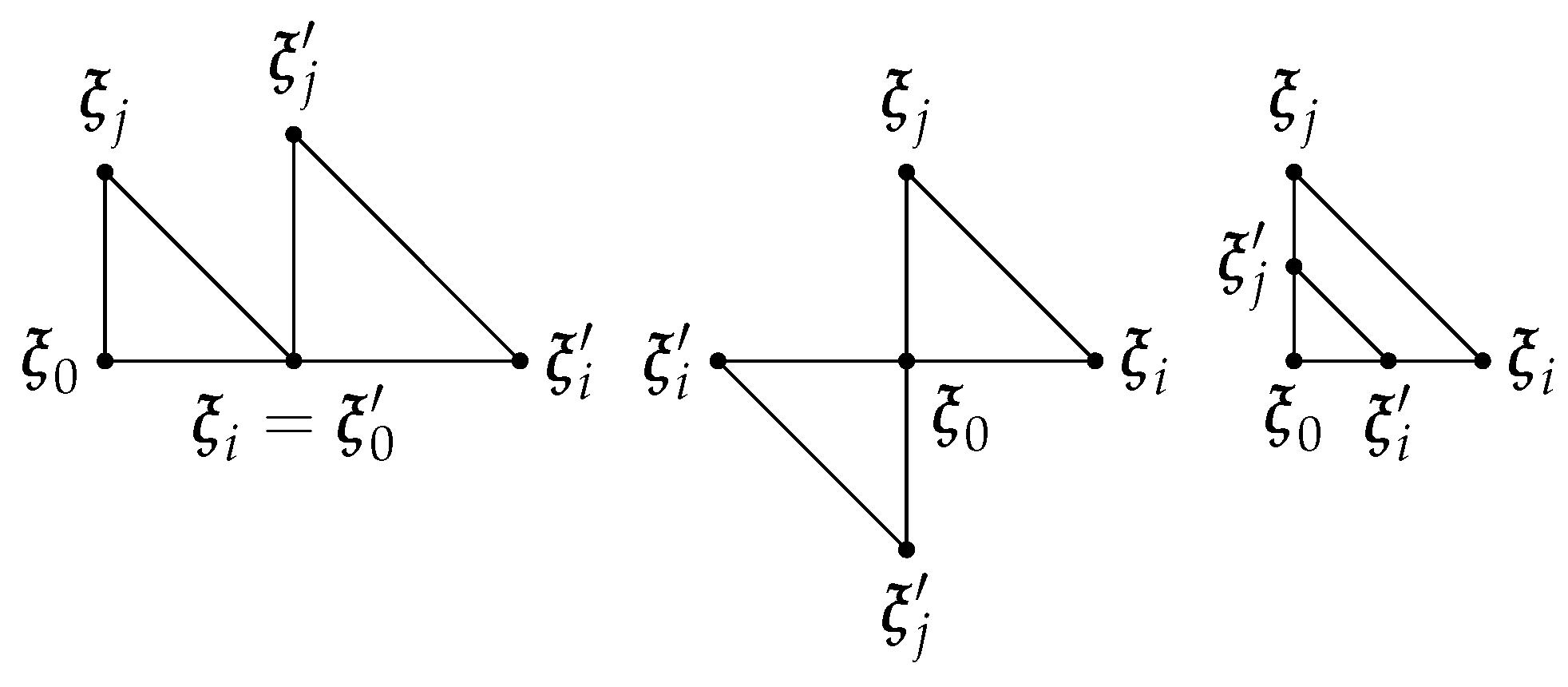
3.2. Review of the Basic Geometric Results about n-Simplices

Let V = { x i : i Z [ 0 , n ] } be a set of n + 1 affinely-independent points in R n , then the closed convex hull of V is an n-simplex Σ with vertex set V , and it is denoted as follows:
Σ = Co ( V )
Next, we introduce certain specific types of n-simplices that are non-standard in the literature.
Definition 1 
(Right n-simplex). A right n-simplex has a vertex, such that the n edges intersecting at it are pairwise orthogonal. This vertex is called the right vertex.
Definition 2 
(Isosceles right n-simplex). A right n-simplex, such that every edge intersecting at the right vertex has the same length Δ, is an isosceles right n-simplex of length Δ.
Definition 3 
(Standard n-simplex). The standard n-simplex is an isosceles right n-simplex of unit length.
By locating the zero of R n in the right vertex, the standard n-simplex Σ n 0 is the n-dimensional polytope with vertex set V = { b i R n : i Z [ 0 , n ] } where b 0 is the zero vector, and b i is the i-th element of the standard basis of R n . Alternatively, the standard n-simplex can be defined as the intersection of the closed unit ball in the one-norm of R n and the non-negative orthant, i.e., Σ n 0 = { x [ 0 , 1 ] n : x 1 1 } .
The content of an n-dimensional object is the measure of the amount of space inside its boundary. For instance, the content of a two-simplex is its area, and the content of a three-simplex is its volume. It can be proven by induction that the content of a standard n-simplex is 1 n ! .
A regular n-box is an n-dimensional box with edges of equal length. If the content of an n-simplex is not zero, then a geometric object of nonzero content can fit in its interior. The following lemma provides the edge length of the maximum regular n-box that can fit in the interior of a standard n-simplex.
Lemma 1. 
The regular n-box of maximum size that can be contained inside a standard n-simplex has edge length 1 n and content 1 n n .
Proof. 
The standard n-simplex is given as Σ n 0 = { x [ 0 , 1 ] n : x 1 1 } . The maximum n-box that can be allocated inside the standard n-simplex has a vertex in the origin, and it is oriented along the coordinate directions. The opposite vertex to the origin of this regular n-box has coordinates x i = 1 n for i Z [ 1 , n ] ; therefore, its edge length is 1 n , and its content is 1 n n . ☐
The edges that intersect at the right vertex of a standard n-simplex are oriented along the coordinate directions, so these edge directions define a nonnegative orthant. Any direction inside this orthant can be expressed by a nonnegative n-dimensional vector of unit norm, i.e., d , d = 1 . A direction d forms angles θ i with the coordinate directions whose cosines are called the directional cosines and are given by cos θ i = d , b i . The following lemma proves that any direction d contained in the nonnegative orthant has at least one directional cosine that never is less than 1 n .
Lemma 2. 
The smallest directional cosine of any direction contained in the orthant formed by the edges intersecting at the right vertex of a standard n-simplex is never less than 1 n .
Proof. 
Without loss of generality, suppose that the right vertex is the zero point and that the edges are in the coordinate directions, characterized by the elements of the standard basis of R n , i.e., b i for i Z [ 0 , n ] . Consider the direction d * = 1 n 1 n whose directional cosines are cos θ i * = d * , b i = 1 n for all i Z [ 1 , n ] . Suppose that unlike the lemma statement, there exists a direction d with unit norm d , d = 1 , such that cos θ i = d , b i < 1 n for all i Z [ 1 , n ] , then d , d < n i Z [ 1 , n ] 1 n = 1 . This contradicts the fact that d has unit norm, and the lemma is proven. ☐
A consequence of this lemma is that any direction contained in the nonnegative n-orthant always forms an angle less than π 2 radians with at least one of the coordinate directions that form the orthant. In addition, if we consider an arbitrary direction d R n , then there always exists an n-simplex similar to the standard n-simplex, such that the edge directions of its right vertex define an orthant, such that the smallest directional cosine is never less than 1 n . This n-simplex is obtained by rotating π radians the edges of the standard n simplex corresponding to the negative components of the direction vector d .

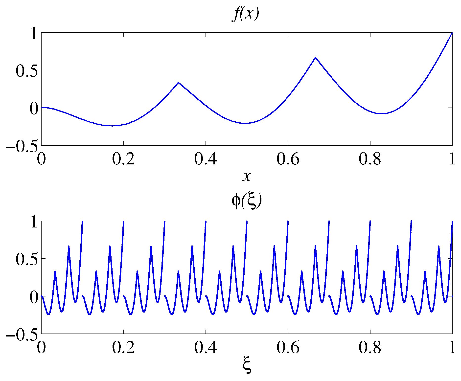
3.3. Function Transformation

A key ingredient of our direct search global optimization algorithm is a transformation of the cost function that improves its exploratory features, providing the capability of jumping out of local minimizers, while preserving termination and convergence properties.
Let x R n be an n-dimensional vector; x denotes the n-dimensional vector whose components are the greatest integers less than or equal to the components of x . The fractional part of x is denoted as frac ( x ) and is defined as follows:
frac ( x ) = x - x
Let ξ be an arbitrary n-dimensional vector of real numbers and P a positive integer. Let us introduce the following map:
x ( ξ ) = frac ( P ξ )
This map is onto and transforms the n-dimensional Euclidean space R n in the n-dimensional unit interval ( 0 , 1 ) n . Let f be the cost function of the minimization problem given in Equation (1) and introduce the following function transformation:
ϕ ( ξ ) : = f ( x ( ξ ) ) = f ( frac ( P ξ ) )
where P is a positive integer. Since the cost function f is not necessarily defined outside of the open unit n-box, the domain of the transformed cost function φ is:
dom ϕ = { ξ R n : P ξ Z n }
The reason is that if P ξ Z n , then frac ( P ξ ) = 0 , and f is not necessarily defined for ξ = 0 .
The transformed function φ has certain interesting properties. The most important are the periodicity of period P - 1 and piecewise continuity, both on each variable.
Lemma 3. 
The transformed function ϕ ( ξ ) = f ( frac ( P ξ ) ) satisfies the following properties:
(i) 
The function φ is continuous for any ξ R n , such that P ξ ( 0 , 1 ) n .
(ii) 
Let ξ , η R n be such that P ξ ( 0 , 1 ) n and P η Z n , then ϕ ( ξ + η ) = ϕ ( ξ ) .
Proof. 
(i) If P ξ ( 0 , 1 ) n , then frac ( P ξ ) = P ξ and ϕ ( ξ ) = f ( P ξ ) . Since f is continuous for any x ( 0 , 1 ) n , then φ is continuous for any ξ R n , such that P ξ ( 0 , 1 ) n ; (ii) If ξ and η are n-dimensional vectors, such that P ξ ( 0 , 1 ) n and P η Z n , respectively, then frac ( P η ) = 0 and frac ( P ( ξ + η ) ) = frac ( P ξ ) = P ξ ; consequently, ϕ ( ξ + η ) = f ( frac ( P ξ ) ) = ϕ ( ξ ) . ☐
Let x R n and B P ( x ) denote the following n-box:
B P ( x ) = { ξ R n : P ξ = P x , P ξ Z n }
The transformed function φ is continuous on B P ( x ) , and there always exists ξ * B P ( x ) , such that ϕ ( ξ * ) = min { ϕ ( ξ ) : ξ dom ϕ } . Note that the n-box B ( x ) is given by B P ( x ) = { ξ = P - 1 ( z + P x ) : z ( 0 , 1 ) n } . If x = 0 , then B P ( 0 ) is the fundamental n-box of the function φ, i.e., B P ( 0 ) = ( 0 , P - 1 ) n . For another x R n , B P ( x ) is an n-box of length P - 1 , where the function φ takes the same values as in the fundamental n-box B P ( 0 ) . Note that there are P n different n-boxes for x ( 0 , 1 ) n ; then, the function φ repeats P n times in the unit n-box ( 0 , 1 ) n .
Example 1. 
The function f ( x ) = | x | - | x sin ( 3 π x ) | , and the transformed function ϕ ( ξ ) = f ( frac ( P ξ ) ) for P = 10 are depicted for the open unit interval in Figure 1. The function f is continuous on the open unit interval ( 0 , 1 ) and has three local minima. The transformed function φ is periodic, of period P - 1 = 0 . 1 , and piecewise continuous on the open unit interval. The fundamental period of φ is B ( 0 ) = ( 0 , 0 . 1 ) , and the function value repeats ten times on the unit interval. The function φ is continuous on each interval B ( x ) = { ξ : 10 ξ = 10 x , 10 ξ Z } for x R , but discontinuous at the boundary points of these intervals, which are given by ξ = 0 . 1 k for any integer k. This discontinuity always occurs if f ( 0 + ϵ ) f ( 1 - ϵ ) for any ϵ > 0 , as occurs in this example and which is clearly visible in Figure 1. Moreover, the function φ is not necessarily defined for these points of discontinuity.
Consider the unconstrained optimization problem:
min { ϕ ( ξ ) : ξ dom ϕ }
The function φ has a global optimizer at ξ * if ϕ ( ξ * ) ϕ ( ξ ) for all ξ dom ϕ . The following theorem proves that the transformed unconstrained minimization problem Equation (12) also provides the minimum value of the original optimization problem Equation (1).
Theorem 1. 
Let f be a real value continuous function on the open unit n-box, and let φ be defined as ϕ ( ξ ) = f ( frac ( P ξ ) ) , where P is a positive integer, then λ * = min { f ( x ) : x ( 0 , 1 ) n } if and only if λ * = min { ϕ ( ξ ) : ξ dom ϕ } .
Proof. 
(If): Let x * be such that λ * = f ( x * ) = min { f ( x ) : x ( 0 , 1 ) n } and ϕ ( ξ ) = f ( frac ( P ξ ) ) , where P is a positive integer; then define ξ * = P - 1 ( x * + η ) for any η Z n ; then ϕ ( ξ * ) = f ( x * ) = λ * . (Only if): Let ξ * be such that λ * = ϕ ( ξ * ) = min { ϕ ( ξ ) : ξ dom ϕ } ; define x * = frac ( P ξ * ) ; then f ( x * ) = ϕ ( ξ * ) = λ * . ☐
Theorem 1 allows us to obtain a global minimizer of the original function f on the open unit n-box by solving the unconstrained optimization problem (12). If we have a method that computes a global minimizer ξ * of the unconstrained optimization problem (12), then x * = frac ( P ξ * ) ( 0 , 1 ) n , and it satisfies ϕ ( ξ * ) = f ( x * ) .
The following lemma proves that any regular n-box of a size greater than or equal to P - 1 always contains a point ξ * that attains the global minimum of the unconstrained optimization problem (12).
Lemma 4. 
Let B be a regular n-box of edge length Δ B , such that P Δ B 1 , and let λ * = min { f ( x ) : x ( 0 , 1 ) } ; then, the n-box B always contains a point ξ * R n , such that ϕ ( ξ * ) = λ * .
Proof. 
Let x * ( 0 , 1 ) n be such that f ( x * ) = λ * f ( x ) for any x ( 0 , 1 ) n , and let ξ ¯ B , such that P ξ ¯ = P ξ ¯ + x * . Consider the open n-box B P ( ξ ¯ ) = { ξ R n : P ξ = P ξ ¯ , P ξ Z n } , then B P ( ξ ¯ ) has edge length P - 1 , and the point ξ * = P - 1 ( x * + P ξ ¯ ) satisfies ξ * B ( ξ ¯ ) B and ϕ ( ξ * ) = f ( x * ) = λ * . ☐
We are also interested in determining the size of an n-simplex similar to the standard n-simplex that always contains a global minimizer of { ϕ ( ξ ) : ξ dom ϕ } . Since Lemma 4 establishes that such a point is always contained in a regular n-box of length not less than P - 1 , then the solution is an isosceles right n-simplex that contains a regular n-box of length P - 1 . From Lemma 1, this n-simplex has edge length n P - 1 and content P - n / ( n - 1 ) ! . The following lemma states the result.
Theorem 2. 
Let Σ be an isosceles right n-simplex of length Δ, such that P Δ n , and let λ * = min { f ( x ) : x ( 0 , 1 ) n } ; then, the n-simplex Σ always contains a point ξ * dom ϕ , such that f ( frac ( ξ * ) ) = λ * .
Proof. 
A regular n-box of edge length Δ B = Δ / n can be inscribed inside any isosceles right n-simplex of length Δ. Since P Δ n , then P Δ B 1 , and the theorem statement is a straightforward consequence of Lemma 4. ☐
In the rest of this section, we shall design a direct search algorithm to obtain a solution for the optimization problem (1). We distinguish two algorithms, the basic algorithm and the complete algorithm. The basic algorithm is a simplex-based algorithm for the transformed cost function. An initial point is embedded at the right vertex of an isosceles right n-simplex of edge length Δ 0 . This n-simplex evolves by a sequence of operations. As a result of each iteration, another n-simplex is obtained that is similar to the standard n-simplex and has the point with minimum value of the transformed cost function located in the right vertex. The edge length of the n-simplex decreases by a constant factor if no operations performed during the iteration produce a vertex with a smaller value of the transformed cost function. Whenever the edge length is no less than n P - 1 , we say that the algorithm is in exploratory phase, because the n-simplex always contains a global minimizer of { ϕ ( ξ ) : ξ dom ϕ } . When the edge length of the n-simplex is less than n P - 1 , then we say that the algorithm is in convergence phase, and it aims to approach a stationary point. Thus, the basic algorithm is designed to preserve the good properties of direct search algorithms, such as convergence to a stationary point, but increases the possibility to reach the global optimum at the end of the exploratory phase. Another feature of the basic algorithm is that there is no interruption or change from one phase to the other, it is a straightforward consequence of using the transformed cost function.

3.4. The Basic Algorithm

The basic algorithm is a simplex-based algorithm for the transformed optimization problem Equation (12). It performs a sequence of operations over an initial simplex until a termination condition is satisfied. The main operators of this algorithm are expansive translation, rotation and shrinkage. The expansive translation is performed after a sufficient decrease of the transformed cost function to ensure that the best point is located at the right vertex. The rotation operation provides exploration of the search space, and the shrinkage operator guarantees termination and global convergence to a stationary point of the transformed cost function. The global improvement is a consequence of using the transformed cost function Equation (8). A sufficient decrease condition of the cost function to accept a successful iteration is a key aspect to prove the termination and global convergence to a stationary point. The main components of the basic algorithm are explained below.

3.4.1. Function Transformation

The cost function transformation is given by:
ϕ ( ξ ) = f ( frac ( P ξ ) )
This transformation aims to perform global improvement at each iteration k Z [ 0 , ) whenever the n-simplex has an edge length, such that P Δ k n .

3.4.2. Initial Simplex

Let vset ( ξ , Δ ) where ξ R n and Δ R be defined as follows:
vset ( ξ , Δ ) : = { ξ i : ξ i = ξ + Δ b i , i Z [ 1 , n ] }
where b 0 is an n-dimensional zero vector and b i for i Z [ 1 , n ] is the i-th element of the standard basis of R n . The initial n-simplex is obtained by varying an initial point at a distance Δ 0 in each coordinate direction, such that P Δ 0 > n . Let ξ 0 ( 0 , 1 ) n be an initial point; then, the vertex set of the initial simplex is given by:
V 0 = vset ( ξ 0 , Δ 0 )
If the initial point ξ 0 is not provided as an input of the algorithm, then it can be randomly chosen. Consequently, the initial simplex is an isosceles right n-simplex with edge length Δ 0 and content 1 n ! Δ 0 n whose right vertex is indexed by zero.

3.4.3. Expansive Translation

This operation aims to position the point with lowest value of the transformed cost function found so far at the right vertex. Let V be the vertex set of an isosceles right n-simplex with edge length Δ, and let ξ i V be such that ϕ ( ξ i ) ϕ ( ξ j ) for ξ j V ; then, the expansive translation of the right n-simplex V with respect to the vertex i is given by the following expression:
ξ j = ξ i + ρ ( ξ j - ξ 0 ) , ξ j V
where 1 ρ < . If the vertex set of the current simplex is given by V = vset ( ξ 0 , Δ ) , then the transformed n-simplex has the vertex set V = vset ( ξ j , Δ ) , where Δ = ρ Δ , and its edge length is | Δ | . The new n-simplex, after the expansive translation, preserves its shape, but increases its content by a factor of ρ n . From a practical point of view, it is convenient to choose the expansive factor ρ close to one, but slightly greater, because this avoids obtaining candidate points that were already visited in previous iterations, in the next rotation operation.
Let c be an arbitrary positive constant; if ϕ ( ξ i ) < ϕ ( ξ 0 ) - c Δ 2 for some ξ i V } , then the algorithm proceeds to a new iteration and performs an expansive translation operation. Otherwise, the algorithm executes a rotation operation.
The introduction of the positive term c Δ 2 guarantees that the iteration is considered successful only if it provides a point with a sufficient decrease of the cost function.

3.4.4. Rotation

This operation produces a similar n-simplex, but where each edge is rotated π radians with respect to the right vertex. A graphical interpretation is depicted in Figure 2.
Let V denote the vertex set of an n-simplex. The vertices of the rotated n simplex are given by the following expression:
ξ j = ξ 0 - ( ξ j - ξ 0 ) , ξ j V
If the vertex set of the current simplex is given by V = vset ( ξ 0 , Δ ) , then the transformed n-simplex has the vertex set V = vset ( ξ 0 , Δ ) , where Δ = - Δ , and its edge length is | Δ | . If ϕ ( ξ i ) < ϕ ( ξ 0 ) - c Δ 2 for some ξ i V , then the rotation operation succeeds, and the algorithm proceeds to start a new iteration and performs an expansive translation operation. Otherwise, the rotation operation fails; the rotated vertex set is discarded; and the algorithm executes a shrinkage operation with the original vertex set V .

3.4.5. Shrinkage

This operation performs a contraction of the simplex by fixing the right vertex and placing the remaining vertices along the same directions, but at a distance that is reduced by a constant factor σ ( 0 , 1 ) . A graphical interpretation of the shrinkage operation is depicted in Figure 2 for R 2 .
Let V denote the vertex set of an n-simplex. The vertices of the transformed n-simplex are given by:
ξ j = ξ 0 + σ ( ξ j - ξ 0 ) , ξ j V
If the vertex set of the current simplex is given by V = vset ( ξ 0 , Δ ) , then the transformed n-simplex has the vertex set V = vset ( ξ 0 , Δ ) , where Δ = σ Δ , and its edge length is | Δ | . After the shrinkage operation, the algorithm proceeds to start a new iteration by performing an expansive translation operation.

3.4.6. Sufficient Decrease Condition

The expansive translation and rotation operations are considered successful if some vertex of the transformed n-simplex satisfies the following sufficient decrease condition:
ϕ ( ξ i ) < ϕ ( ξ 0 ) - c Δ 2 , for some ξ i V
where c is a positive constant. This condition is key to proving the termination of the basic algorithm and global convergence to a stationary point. The constant c is arbitrary, but usually, a small value is chosen.

3.4.7. Stopping Criterion

The sufficient decrease condition and the shrinkage operation guarantee that the size of the n-simplex converges to zero. Consequently, a stopping criterion can be defined by taking a sufficiently small number ϵ > 0 . Let | Δ | be the edge length of the n-simplex; then, the basic algorithm stops when the following condition is satisfied:
P | Δ | ϵ

3.4.8. Space Transformation

The search space transformation is given by the map:
x ( ξ ) = frac ( P ξ )
Therefore, when the n-simplex with vertex set V reaches edge length Δ ϵ , the basic algorithm stops, and the point obtained is x ¯ = frac ( P ξ ¯ ) , where ξ ¯ arg min { ξ : ξ V } ; and it attains the function value f ( x ¯ ) = ϕ ( ξ ¯ ) .

3.4.9. Implementation

An implementation of the basic algorithm in pseudocode is given in Algorithm 1.
Algorithm 1 Basic algorithm.
1:
function BGDS( f , x 0 )
2:
    parameters: ϵ > 0 , P N
3:
    definitions: s ( ξ ) : = P ξ - P ξ , ϕ ( ξ ) : = f ( s ( ξ ) )
4:
     z rand ( dim ( x 0 ) )
5:
     ξ 0 ( P z + x 0 ) / P
6:
     ϵ ϵ / P
7:
     ξ LDS ( ϕ , ξ 0 , ϵ )
▹ Local direct search
8:
    return s ( ξ )
9:
end function
10:
function LDS( ϕ , ξ 0 , ϵ )
11:
    parameters: ρ , σ , c R : 1 ρ , 0 < σ < 1 , 0 < c , 0 < Δ
12:
    definitions: vset ( ξ , Δ ) : = ξ R n , Δ R } , vmin ( V ) arg min { ϕ ( ξ i ) : ξ i V }
13:
     ξ ξ 0
14:
     V vset ( ξ , Δ )
15:
     ξ min vmin ( V )
16:
    while ϵ < | Δ | do
17:
        if ϕ ( ξ min ) < ϕ ( ξ ) - c Δ 2 then
▹ Expansive translation
18:
            ξ ξ min
19:
            Δ ρ Δ
20:
            V vset ( x , Δ )
21:
            ξ min vmin ( V )
22:
        end if
23:
        if ϕ ( ξ ) - c Δ 2 ϕ ( ξ min ) then
▹ Rotation
24:
            Δ - Δ
25:
            V vset ( ξ , Δ )
26:
            ξ min vmin ( V )
27:
        end if
28:
        if ϕ ( ξ ) - c Δ 2 ϕ ( ξ min ) then
▹ Shrinkage
29:
            Δ σ Δ
30:
            V vset ( ξ , Δ )
31:
            ξ min vmin ( V )
32:
        end if
33:
    end while
34:
    return ξ min
35:
end function

3.5. Convergence of the Basic Algorithm

The basic algorithm has been designed to provide termination and improvement by performing a sequence of simplex transformations. If in addition, the cost function is differentiable and its gradient is Lipschitz continuous, then the basic algorithm converges to a stationary point.
Theorem 3. 
Let f be the cost function of a minimization problem on the open unit n-box; then the basic algorithm always terminates. If, in addition, f is differentiable and its gradient Δ f is Lipschitz continuous on the unit n-box, then the sequence of points generated at each iteration by the basic algorithm converges to a stationary point.
Proof. 
Let S and U denote the index sets of successful and unsuccessful iterations of the basic algorithm, respectively. Let x k = frac ( P ξ k ) , then f ( x k ) = ϕ ( ξ k ) . If k S , then f ( x k + 1 ) < f ( x k ) - c Δ k 2 and Δ k + 1 = ρ Δ k , while if k U , then f ( x k + 1 ) f ( x k ) - c Δ k 2 and Δ k + 1 = σ Δ k . Let us begin by proving that lim k | Δ k | = 0 . Suppose not; then, for any k Z [ 0 , ] , there exists k , such that S because, if such an does not exist, then the set of successful iterations would be finite, and when k approaches infinity, the update rule Δ k + 1 = σ Δ k yields lim k | Δ k | = 0 . In addition, there exists Δ ¯ > 0 , such that for each successful iteration S , | Δ | Δ ¯ and:
f ( x + 1 ) < f ( x ) - c Δ 2 f ( x ) - c Δ ¯ 2
However, since approaches infinity, this implies that f ( x + 1 ) - , which contradicts the fact that the function f is bounded below on ( 0 , 1 ) n . Consequently, the boundedness of f implies that Δ ¯ = 0 and lim k | Δ k | = 0 . This proves the termination of the basic algorithm.
For the second part of the theorem, if f is continuous and differentiable on ( 0 , 1 ) n , then so is ϕ ( ξ ) = f ( frac ( P ξ ) ) on the n-box B P ( x ) = { ξ R n : P ξ = P x , P ξ Z n } for any x R n . Furthermore, if f is Lipschitz continuous with constant M on ( 0 , 1 ) n , then so is ϕ in B P ( x ) with constant P M . Since we proved that lim k | Δ k | = 0 , then there always exists a positive integer L, such that P ξ k = P ξ L for any positive integer k > L . The basic algorithm searches points along the coordinate directions; then, from Lemma 2 and for any positive integer k > L , no matter the value of ϕ ( ξ k ) , there is always at least one (positive or negative) coordinate direction d i { b i , - b i } , such that:
1 n cos θ = - ϕ ( ξ k ) , b i ϕ ( ξ k ) d i
or equivalently:
1 n ϕ ( ξ k ) - ϕ ( ξ k ) , d i
because d i = 1 . For any unsuccessful iteration k U , ϕ ( ξ k + | Δ k | d k ) ϕ ( ξ k ) - c Δ k 2 , the mean value theorem establishes that:
- c Δ k 2 ϕ ( ξ k + | Δ k | d i ) - ϕ ( ξ k ) = ϕ ( ξ k + α k | Δ k | d i ) , d i | Δ k |
for some α k [ 0 , 1 ] . Subtracting ϕ ( ξ k ) , d i | Δ k | from both sides leads to:
- c Δ k 2 - ϕ ( ξ k ) , d i | Δ k | ϕ ( ξ k + α k | Δ k | d i ) - ϕ ( ξ k ) , d i | Δ k |
Applying Equation (21) yields:
1 n ϕ ( ξ k ) ϕ ( ξ k + α k | Δ k | d i ) - ϕ ( ξ k ) , d i + c | Δ k |
Taking into account that φ is continuously differentiable in B P ( ξ k ) and its gradient ϕ is Lipschitz with constant P M in B P ( ξ k ) ,
1 n ϕ ( ξ k ) P M α k Δ k d i + c | Δ k | ( P M + c ) | Δ k |
because α k ( 0 , 1 ) and b i = 1 . Consequently,
ϕ ( ξ k ) n ( P M + c ) | Δ k |
and taking the limit when k approaches infinity, it is possible to conclude that:
lim k ϕ ( ξ k ) n ( P M + c ) lim k | Δ k | = 0 , for k U
and finally, by making x k = frac ( ξ k ) :
lim k f ( x k ) = P lim k ϕ ( ξ k ) = 0 , for k U .
Consequently, the sequence of points generated by the basic algorithm converges to a stationary point. ☐
Remark 2. 
The basic algorithm can be applied to any cost function f, not necessarily continuous or differentiable in the search space ( 0 , 1 ) n . For a continuous and differentiable function with a Lipschitz continuous gradient, the basic algorithm converges to a stationary point. If in addition the cost function is strictly convex, then the unique optimizer is a stationary point, and Theorem 3 guarantees that the basic algorithm converges to the unique optimizer. Note that we do not need to know the value of the Lipschitz constant M.
Example 2. 
The evolution of the basic algorithm for the function f ( x ) = | x | - | x sin ( 3 π x ) | is depicted in Figure 3. The parameters of the algorithm are P = 10 4 , σ = 0 . 5 , ρ = 1 . 05 , c = 0 . 01 , ϵ = 10 - 4 . Since this problem is unidimensional, the simplex is an interval. The left plots represent the vertex points of the simplex in the original space (above) and their corresponding function values (below) after each iteration. The right plots represent the values of the worst (above) and best (below) points of the simplex in the original space that were obtained during the execution of the algorithm. Note that the algorithm explores the whole range of the unit interval. This exploration is performed whenever the length of the simplex edge Δ k satisfies P Δ k 1 , which corresponds to the exploratory phase of the algorithm. Once Δ k is P Δ k < 1 , then the algorithm enters the phase of convergence to a stationary point. In this example, the algorithm stops after 24 iterations. From Iterations 1 to 12, the algorithm is in the exploratory phase, and from Iterations 13 to 24, the algorithm is in the convergence phase to a stationary point. The point obtained corresponds to f ( 0 . 1721 ) = - 0 . 2422 , which is the global minimal value within the space tolerance ϵ.

3.6. The Complete Algorithm

The complete algorithm, that we call GDS (an acronym for Global Direct Search), is obtained by repeating the basic algorithm a number of times. A single application of the basic algorithm may obtain the global optimum within a space tolerance ϵ only in easy problems. For more difficult optimization problems, a new execution of the basic algorithm, starting with the best point obtained in the previous execution, may improve the result. Each execution produces a local minimizer; however, if there are better points in some coordinate direction, the algorithm may jump to one of these points during the exploratory phase of a new execution. Unfortunately, not every optimization problem satisfies the property that, for any local minimizer, there are points in some coordinate direction where the cost function is improved. In such a case, a strategy that turns out to be more effective is to start from a new random initial point. The class of cost functions that we are facing is not usually known in advance, and we do not know which strategy is more appropriate for a new execution of the basic algorithm. A trade-off solution is to repeat the basic algorithm N times, but starting from a new random initial point after a number R N of repetitions.

3.6.1. Initial Point

Let N denote the total number of executions of the basic algorithm and R the number of repetitions without choosing a new initial point. Let x ¯ denote the point obtained in the previous execution of the basic algorithm and ξ r a random vector in ( 0 , 1 ) n with a uniform probability distribution. The initial point for the n-th execution of the basic algorithm is obtained as follows:
ξ 0 = frac ( P - 1 int ( P ξ r ) + x ¯ ) if n mod ( R + 1 ) 0 ξ r if n mod ( R + 1 ) = 0
where mod is the modulo operator that represents the remainder of the integer division of their arguments. Note that if R = 0 , the initial point is always a random point; however, if R = N , the initial point is always the point obtained in the previous execution of the basic algorithm.

3.6.2. Best Point Storage

The minimum point found during the execution of the complete algorithm is preserved. The point obtained after each basic algorithm execution is compared to the best solution stored and, in the case of improvement, the new point replaces it. Let x denote the point obtained after the last execution of the basic algorithm and x min the best point stored so far; the storage rule is:
x min = x ¯ if f ( x ¯ ) < f ( x min ) x min otherwise

3.6.3. Implementation of the Complete Algorithm

An implementation of the complete algorithm GDS in pseudocode is given in Algorithm 2.
Algorithm 2 Complete algorithm GDS.
1:
function GDS( f , x 0 )
2:
    parameters: N , R N , such that R N
3:
     x min x 0
4:
    for k = 1 to N do
5:
         x x min
6:
        if k mod ( R + 1 ) = 0 then
7:
            x rand ( dim ( x 0 ) )
8:
        end if
9:
         x BGDS ( f , x )         ▹ Basic global direct search
10:
        if f ( x ) < f ( x min ) then
11:
            x min x
12:
        end if
13:
    end for
14:
    return x min
15:
end function

4. Experimental Study

4.1. Test Functions

Global optimization is not a trivial problem. Theoretical results, such as the No Free Lunch (NFL) theorem [61], state that an efficient general-purpose universal optimization algorithm is not possible. In other words, this result says that one algorithm can outperform another only for a certain class of problems. It is a usual practice to analyze the performance of an optimization algorithm by using test functions. A large number of standard test functions have been used to study the performance of our direct search global optimization algorithm. In this section, we present the results for the 24 functions given in Table 1. These function are described in detail in [62]. The functions are classified into five groups: separable functions (func # 1.xx), functions with low or moderate conditioning (func # 2.xx), unimodal functions with high conditioning (func # 3.xx), multimodal functions with an adequate global structure (func # 4.xx) and multimodal functions with a weak global structure (func # 5.xx). All of the functions are scalable with the dimension. All of the functions are defined and can be evaluated over R n , and the search space is [ - 5 , 5 ] n , where n is the dimension of the function domain. The global optimal value is attained in this search space.

4.2. Selection of the GDS Parameters

The performance of the GDS algorithm for different parameter values has been empirically analyzed by means of extensive computer studies. Our algorithm has been implemented in the scientific software MATLAB [63], and its performance has been successfully compared to the global optimization strategies that are implemented in the Global Optimization Toolbox of MATLAB. The GDS algorithm has a number of configurable parameters, and this comparative study allowed us to select a set of parameters that are appropriate for many problems. The expansive and contractive factors are set to ρ = 1 . 05 and σ = 0 . 5 . It is convenient to take the expansive value slightly greater than one to avoid evaluating points already checked in previous iterations. However, large values of ρ usually produce slow convergence. Consequently, values in the interval [ 1 . 01 , 1 . 10 ] are usually a good option for most problems. Regarding the contractive factor σ, the closer to one, the larger the number of iterations of the basic GDS algorithm will be. From our experiments, σ = 0 . 5 is a convenient value that produces a satisfactory trade-off between the efficiency of the algorithm and the convergence time. The constant c of the sufficient decrease condition is chosen as c = 0 . 01 . Any positive value of c provides the termination of the algorithm, but small values are recommended to improve the algorithm’s performance during the initial iterations when Δ is large. The parameters P and R were fixed to P = 1000 and R = 5 . These values were selected after a massive experimentation. In our experiments, we analyzed the mean value of the CPU time for one execution of the basic GDS algorithm for different values of the parameter R. The empirical results showed that the larger the value of R, the lower the CPU time for execution. This means that when R increases, the number of executions N can also be increased to a certain extent without compromising the total CPU time. The reduction is larger for smaller values of R, e.g., the reduction is about 40% from R = 0 to R = 1 and about 30% from R = 1 to R = 2 . Since increasing R is also beneficial for functions that can be globally optimized along the coordinate directions, a good option that trades off between moderate CPU time and efficiency in computing the global optimum is to choose R [ 2 , 10 ] and increase the number of repetitions of the basic algorithm N as much as possible, to maintain a moderate total CPU time. In fact, we have checked that a good selection of P and R could improve the results depending on the problem. However, since a practitioner usually does not know in advance what class its problem belongs to, it is important to fix a set of parameters that trade off for a large class of problems. In conclusion, the parameter values of the GDS algorithm for the experimental study were selected as P = 1000 , R = 5 , ρ = 1 . 05 , σ = 0 . 5 , c = 0 . 01 and N = 1 e 9 , and the stopping criterion is the number of function evaluations.

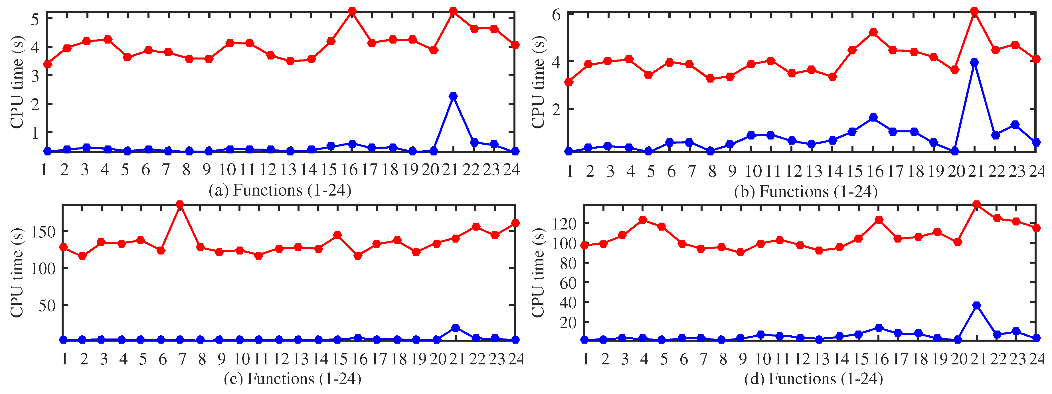
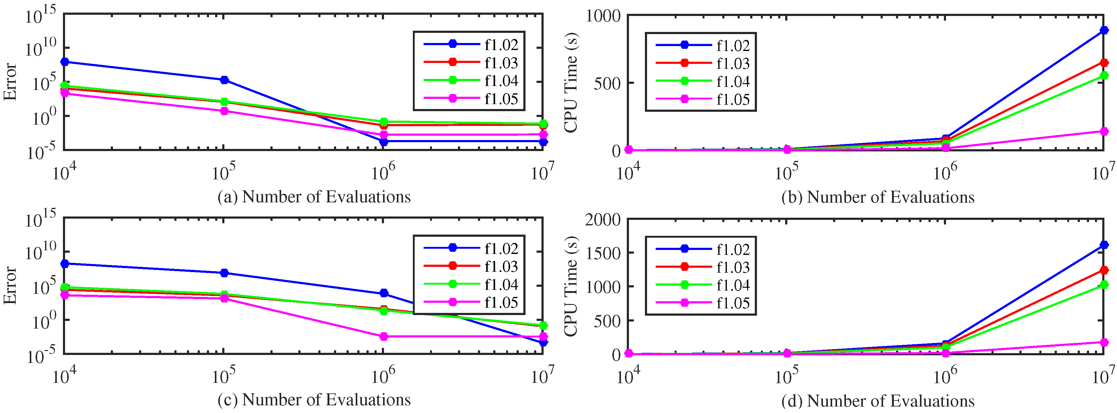
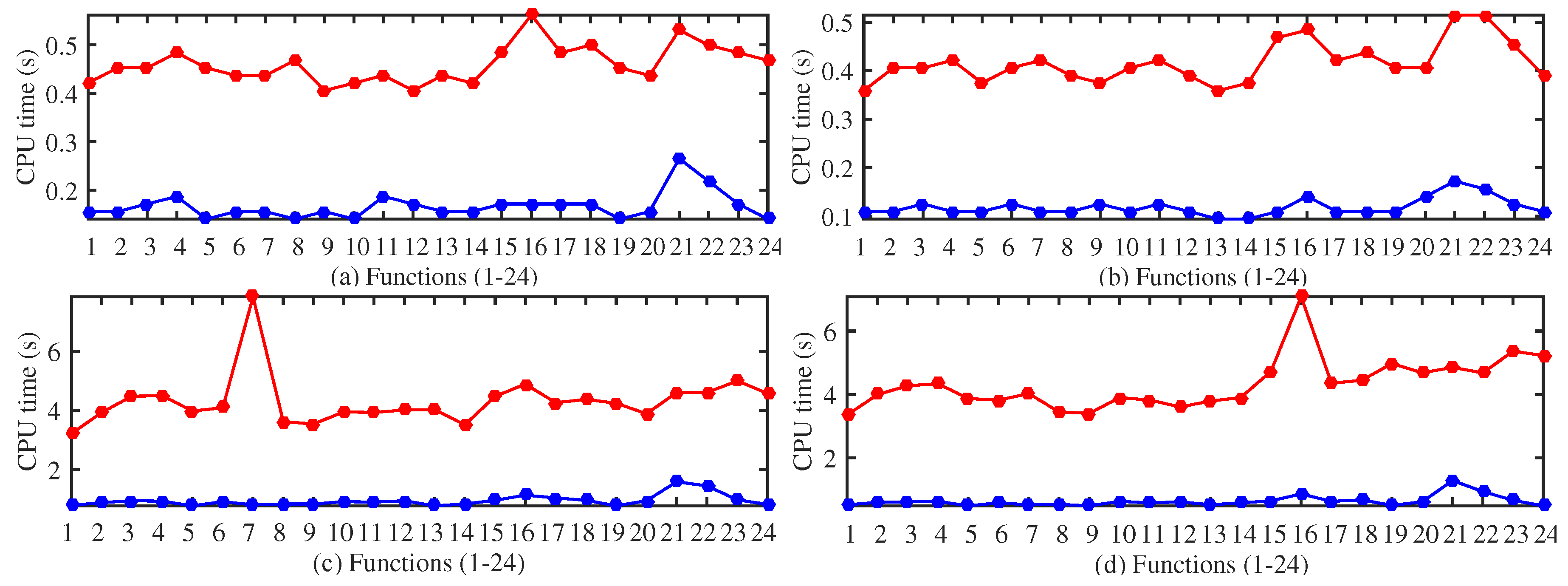
4.3. Performance Evaluation

The evaluation of the GDS algorithm has been accomplished by solving the 24 functions in Table 1 using the fixed set of parameters values explained in the previous subsection. The performance of GDS is compared to DIRECT [51]. DIRECT is a deterministic global optimization algorithm based on the domain partition strategy. Each iteration includes two phases. The first phase identifies hyper-rectangles that potentially contain a global optima. In the second phase, the hyper-rectangles identified in the first phase are partitioned into smaller hyper-rectangles, and the cost function is evaluated at the centers of the hyper-rectangles. The convergence properties guarantee that if no termination criteria are included, DIRECT will exhaustively sample the domain. The implementation of DIRECT in MATLAB by Finkel [64] has been used in this study. The experiments have been performed in a laptop PC equipped with a dual core processor Intel (R) Core (TM) i5-3317U CPU @1.70 GHz running MATLAB R2014a under the Windows operating system.
The comparative study has been performed as follows: For both algorithms, GDS and DIRECT, a fixed number of function evaluations is used as a stopping condition, and the error in computing the global minimum value is obtained. Each problem has been solved 15 times, and the median of the error is tabulated for each function. The study has been accomplished for the 24 functions of Table 1 and for different dimensions of the function domain and different numbers of function evaluations. The default parameters of DIRECT [64] have been used, but using the number of function evaluations as stopping conditions.
In Table 2, the results for functions of dimensions five and 10 and a number of function evaluations equal to 10 3 and 10 4 are shown, while in Table 3, the same results are shown for dimensions 10 and 20 and 10 4 and 10 5 function evaluations. GDS and DIRECT obtained different results for different functions. In general, for a small number of function evaluations, DIRECT gets a smaller median of the error. However, as the number of function evaluations increases, the improvement in approaching the minimum value is higher in GDS. One of the outstanding features of GDS is its simplicity. This can be checked by comparing the CPU time with DIRECT. The CPU time for all of the problems, dimensions and function evaluations is much smaller for GDS; see Figure 4 and Figure 5. Note that GDS is more than 100-times faster than DIRECT for several functions of dimension 40 and 10 5 function evaluations.
The results of a study of the GDS algorithm for functions of high dimension are presented in Figure 6. The GDS algorithm is executed on the functions 1.02, 1.02, 1.04 and 1.05 of dimensions 100 and 200 to search the global minimum. The error to the global minimum in the logarithmic scale and the CPU time are shown for 10 4 , 10 5 , 10 6 and 10 7 . It is interesting to remark that the CPU time grows linearly with the dimension of the problem.
Since GDS is simple and computationally efficient, it can be successfully applied to problems of high dimensions where the number of function evaluations to obtain a good result is large for any direct search algorithm.

5. Conclusions

A direct search algorithm for the global optimization of multivariate functions has been reported. The algorithm performs a sequence of operations for an initial isosceles right n-simplex. The result of these operations is always a similar n-simplex of a different size. The operations depend on the values of the vertices of the n-simplex, where these values are computed using a transformed cost function that improves the exploratory features of the algorithm. The convergence properties of the algorithm have been proven. The results of an extensive experimental study demonstrate that the algorithm is capable of approaching the global optimum for black box problems with moderate computation time. It is competitive with most of the heuristic-based global optimization strategies presently used. Furthermore, it has been compared to DIRECT, a well-known Lipschitzian-based direct search algorithm. The new algorithm is very simple and computationally cost-effective and can be applied to problems of high dimension, because the empirical results demonstrate that its computation time increases linearly with the dimension of the problem. In future work, we plan to extend the algorithm to constrained optimization.

Acknowledgments

The authors thank Instituto de las Tecnologías Avanzadas de la Producción (ITAP) for supporting the publication costs.

Author Contributions

Enrique Baeyens and Alberto Herreros design the GDS algorithm and develop the experiments. José R. Perán analyzed the results. The three autors contributed equally to writing the paper.

Conflicts of Interest

The authors declare no conflict of interest.

References

  1. Lewis, R.M.; Torczon, V.; Trosset, M.W. Direct Search Methods: Then and Now. J. Comput. Appl. Math. 2000, 124, 191–207. [Google Scholar] [CrossRef]
  2. Cohn, A.; Scheinberg, K.; Vicente, L. Introduction to Derivative-Free Optimization; MOS/SIAM Series on Optimization; SIAM: Philadelphia, PA, USA, 2009. [Google Scholar]
  3. Pinter, J.D. Global Optimization: Software, Test Problems, and Applications. In Handbook of Global Optimization; Pardalos, P.M., Romeijn, H.E., Eds.; Kluwer Academic Publishers: Dordrecht, The Netherlands, 2002; Volume 2. [Google Scholar]
  4. Kolda, T.G.; Lewis, R.M.; Torczon, V. Optimization by Direct Search: New Perspectives on Some Classical and Modern Methods. SIAM Rev. 2003, 45, 385–482. [Google Scholar] [CrossRef]
  5. Neumaier, A. Complete Search in Continuous Global Optimization and Constraint Satisfaction. Acta Numer. 2004, 13, 271–369. [Google Scholar] [CrossRef]
  6. Conn, A.R.; Scheinberg, K.; Vicente, L.N. Introduction to Derivative-Free Optimization; SIAM: Philadelphia, PA, USA, 2009; Volume 8. [Google Scholar]
  7. Rios, L.M.; Sahinidis, N.V. Derivative-free optimization: A review of algorithms and comparison of software implementations. J. Glob. Optim. 2013, 56, 1247–1293. [Google Scholar] [CrossRef]
  8. Swann, W.H. Direct Search Methods. In Numerical Methods for Unconstrained Optimization; Murray, W., Ed.; Academic Press: Salt Lake City, UT, USA, 1972; pp. 13–28. [Google Scholar]
  9. Evtushenko, Y.G. Numerical methods for finding global extrema (case of a non-uniform mesh). USSR Comput. Math. Math. Phys. 1971, 11, 38–54. [Google Scholar] [CrossRef]
  10. Strongin, R. A simple algorithm for searching for the global extremum of a function of several variables and its utilization in the problem of approximating functions. Radiophys. Quantum Electron. 1972, 15, 823–829. [Google Scholar] [CrossRef]
  11. Sergeyev, Y.D.; Strongin, R. A global minimization algorithm with parallel iterations. USSR Comput. Math. Math. Phys. 1989, 29, 7–15. [Google Scholar] [CrossRef]
  12. Dennis, J.E.J.; Torczon, V. Direct Search Methods On Parallel Machines. SIAM J. Optim. 1991, 1, 448–474. [Google Scholar] [CrossRef]
  13. Hooke, R.; Jeeves, T. Direct search solution of numerical and statistical problems. J. ACM 1961, 8, 12–229. [Google Scholar] [CrossRef]
  14. Nelder, J.A.; Mead, R. A Simplex Method for Function Minimization. Comput. J. 1965, 7, 308–313. [Google Scholar] [CrossRef]
  15. Spendley, W.; Hext, G.R.; Himsworth, F.R. Sequential Application of Simplex Designs in Optimisation and Evolutionary Operation. Technometrics 1962, 4, 441–461. [Google Scholar] [CrossRef]
  16. Lagarias, J.; Reeds, J.; Wright, M.; Wright, P. Convergence Properties of the Nelder-Mead Simplex Method in Low Dimensions. SIAM J. Optim. 1998, 9, 112–147. [Google Scholar] [CrossRef]
  17. Conn, A.; Gould, N.; Toint, P. Trust-Region Methods; Society for Industrial and Applied Mathematics: Philadelphia, PA, USA, 2000. [Google Scholar]
  18. Regis, R.; Shoemaker, C. Constrained global optimization of expensive black box functions using radial basis functions. J. Glob. Optim. 2005, 31, 153–171. [Google Scholar] [CrossRef]
  19. Custodio, A.; Rocha, H.; Vicente, L. Incorporating minimum Frobenius norm models in direct search. Comput. Optim. Appl. 2010, 46, 265–278. [Google Scholar] [CrossRef]
  20. Conn, A.; Le Digabel, S. Use of quadratic models with mesh-adaptive direct search for constrained black box optimization. Optim. Methods Softw. 2013, 28, 139–158. [Google Scholar] [CrossRef]
  21. Lewis, R.; Torczon, V. Pattern search algorithms for bound constrained minimization. SIAM J. Optim. 1999, 9, 1082–1099. [Google Scholar] [CrossRef]
  22. Lewis, R.; Torczon, V. Pattern search algorithms for linearly constrained minimization. SIAM J. Optim. 2000, 10, 917–941. [Google Scholar] [CrossRef]
  23. Lewis, R.; Torczon, V. A globally convergent augmented Lagrangian pattern search algorithm for optimization with general constraints and simple bounds. SIAM J. Optim. 2002, 12, 1071–1089. [Google Scholar] [CrossRef]
  24. Kolda, T.; Lewis, R.; Torczon, V. A Generating Set Direct Search Augmented Lagrangian Algorithm for Optimization with a Combination of General and Linear Constraints; Sandia National Laboratories: Livermore, CA, USA, 2006.
  25. Audet, C.; Dennis, J.E. A pattern search filter method for nonlinear programming without derivatives. SIAM J. Optim. 2004, 14, 980–1010. [Google Scholar] [CrossRef]
  26. Abramson, M.; Audet, C.; Dennis, J. Filter pattern search algorithms for mixed variable constrained optimization problems. Pac. J. Optim. 2007, 3, 477–500. [Google Scholar]
  27. Dennis, J.; Price, C.; Coope, I. Direct search methods for nonlinearly constrained optimization using filters and frames. Optim. Eng. 2004, 5, 123–144. [Google Scholar] [CrossRef]
  28. Solis, F.J.; Wets, R.J.B. Minimization by Random Search Techniques. Math. Oper. Res. 1981, 6, 19–30. [Google Scholar] [CrossRef]
  29. Pearl, J. Heuristics: Intelligent Search Strategies for Computer Problem Solving; Addison-Wesley Longman Publishing Co., Inc.: Boston, MA, USA, 1984. [Google Scholar]
  30. Michalewicz, Z.; Fogel, D.B. How to Solve It: Modern Heuristics, 2nd ed.; Springer: Berlin, Germany, 2004. [Google Scholar]
  31. Kirkpatrick, S.; Gelatt, C.D.; Vecchi, M.P. Optimization by Simulated Annealing. Science 1983, 220, 671–680. [Google Scholar] [CrossRef] [PubMed]
  32. Bäck, T. Evolutionary Algorithms in Theory and Pratice; Oxford University Press: New York, NY, USA, 1996. [Google Scholar]
  33. Larrañaga, P.; Lozano, J.A. Estimation of Distribution Algorithms: A New Tool for Evolutionary Computation; Kluwer: Boston, MA, USA, 2002. [Google Scholar]
  34. Kennedy, J.; Eberhart, R. Particle Swarm Optimization. In Proceedings of the 1995 IEEE International Conference on Neural Networks, Perth, Australia, 27 November–1 December 1995; Volume 4, pp. 1942–1948.
  35. Poli, R.; Kennedy, J.; Blackwell, T. Particle swarm optimization. Swarm Intell. 2007, 1, 33–57. [Google Scholar] [CrossRef]
  36. Storn, R.; Price, K. Differential Evolution—A Simple and Efficient Heuristic for global Optimization over Continuous Spaces. J. Glob. Optim. 1997, 11, 341–359. [Google Scholar] [CrossRef]
  37. Chakraborty, U.K. Advances in Differential Evolution; Springer Publishing Company: Berlin, Germany, 2008. [Google Scholar]
  38. Glover, F. Tabu Search—Part I. ORSA J. Comput. 1989, 2, 190–206. [Google Scholar] [CrossRef]
  39. Glover, F.; Laguna, M. Tabu Search; Kluwer Academic Publishers: New York, NY, USA, 1997. [Google Scholar]
  40. Dorigo, M.; Maniezzo, V.; Colorni, A. Ant system: Optimization by a colony of cooperating agents. IEEE Trans. Syst. Man Cybern. Part B Cybern. 1996, 26, 29–41. [Google Scholar] [CrossRef] [PubMed]
  41. Dorigo, M.; Stützle, T. Ant Colony Optimization; Bradford Company: Scituate, MA, USA, 2004. [Google Scholar]
  42. Paulavičius, R.; Žilinskas, J. Simplicial Global Optimization; Springer: Berlin, Germany, 2014. [Google Scholar]
  43. Sergeyev, Y.D.; Strongin, R.G.; Lera, D. Introduction to Global Optimization Exploiting Space-Filling Curves; Springer: Berlin, Germany, 2013. [Google Scholar]
  44. Strongin, R.G.; Sergeyev, Y.D. Global Optimization with Non-Convex Constraints: Sequential and Parallel Algorithms; Springer: Berlin, Germany, 2013. [Google Scholar]
  45. Zhigljavsky, A.; Žilinskas, A. Stochastic Global Optimization; Springer: Berlin, Germany, 2008. [Google Scholar]
  46. Zhigljavsky, A.A. Theory of Global Random Search; Springer: Berlin, Germany, 2012. [Google Scholar]
  47. Shubert, B.O. A sequential method seeking the global maximum of a function. SIAM J. Numer. Anal. 1972, 9, 379–388. [Google Scholar] [CrossRef]
  48. Sergeyev, Y.D.; Kvasov, D.E. Global search based on efficient diagonal partitions and a set of Lipschitz constants. SIAM J. Optim. 2006, 16, 910–937. [Google Scholar] [CrossRef]
  49. Lera, D.; Sergeyev, Y.D. Lipschitz and Hölder global optimization using space-filling curves. Appl. Numer. Math. 2010, 60, 115–129. [Google Scholar] [CrossRef]
  50. Kvasov, D.E.; Sergeyev, Y.D. Lipschitz global optimization methods in control problems. Autom. Remote Control 2013, 74, 1435–1448. [Google Scholar] [CrossRef]
  51. Jones, D.R.; Perttunen, C.D.; Stuckman, B.E. Lipschitzian optimization without the Lipschitz constant. J. Optim. Theory Appl. 1993, 79, 157–181. [Google Scholar] [CrossRef]
  52. Gablonsky, J.M.; Kelley, C.T. A locally-biased form of the DIRECT algorithm. J. Glob. Optim. 2001, 21, 27–37. [Google Scholar] [CrossRef]
  53. Finkel, D.E.; Kelley, C. Additive scaling and the DIRECT algorithm. J. Glob. Optim. 2006, 36, 597–608. [Google Scholar] [CrossRef]
  54. Paulavičius, R.; Sergeyev, Y.D.; Kvasov, D.E.; Žilinskas, J. Globally-biased Disimpl algorithm for expensive global optimization. J. Glob. Optim. 2014, 59, 545–567. [Google Scholar] [CrossRef]
  55. Liu, Q.; Cheng, W. A modified DIRECT algorithm with bilevel partition. J. Glob. Optim. 2014, 60, 483–499. [Google Scholar] [CrossRef]
  56. Ge, R.P. The theory of filled function-method for finding global minimizers of nonlinearly constrained minimization problems. J. Comput. Math. 1987, 5, 1–9. [Google Scholar]
  57. Ge, R.; Qin, Y. The globally convexized filled functions for global optimization. Appl. Math. Comput. 1990, 35, 131–158. [Google Scholar] [CrossRef]
  58. Han, Q.; Han, J. Revised filled function methods for global optimization. Appl. Math. Comput. 2001, 119, 217–228. [Google Scholar] [CrossRef]
  59. Liu, X.; Xu, W. A new filled function applied to global optimization. Comput. Oper. Res. 2004, 31, 61–80. [Google Scholar] [CrossRef]
  60. Zhang, Y.; Zhang, L.; Xu, Y. New filled functions for nonsmooth global optimization. Appl. Math. Model. 2009, 33, 3114–3129. [Google Scholar] [CrossRef]
  61. Wolpert, D.; Macready, W. No Free Lunch Theorems for Optimization. IEEE Trans. Evol. Comput. 1997, 1, 67–82. [Google Scholar] [CrossRef]
  62. Hansen, N.; Finck, S.; Ros, R.; Auger, A. Real-Parameter Black-Box Optimization Benchmarking 2009: Noiseless Functions Definitions; Research Report RR-6829; INRIA: Rocquencourt, France, 2009. [Google Scholar]
  63. Mathworks. MATLAB User’s Guide (R2010a); The MathWorks, Inc.: Natick, MA, USA, 2010. [Google Scholar]
  64. Finkel, D.E. DIRECT Optimization Algorithm User Guide; Center for Research in Scientific Computation, North Carolina State University: Raleigh, NC, USA, 2003. [Google Scholar]
Figure 1. A continuous function f ( x ) = | x | - | x sin ( 3 π x ) | with three local minima in the unit interval ( 0 , 1 ) and the corresponding transformed function ϕ ( ξ ) : = f ( frac ( P ξ ) ) where P = 10 for the same interval.
Algorithms 09 00040 g001
Figure 2. Graphical representation of the simplex translation, rotation and shrinking simplex operations for three points in R 2 . The initial vertex set is V = { ξ 0 , ξ i , ξ j } , and the final vertex set is V = { ξ 0 , ξ i , ξ j } . The three operations produce similar simplices.
Algorithms 09 00040 g002
Figure 3. Evolution of the algorithm for f ( x ) = | x | - | x sin ( 3 π x ) | and x ( ξ ) = frac ( P ξ ) . The parameters of the algorithm are P = 10 4 , σ = 0 . 5 , ρ = 1 . 05 , c = 0 . 01 , ϵ = 10 - 4 / P .
Algorithms 09 00040 g003
Figure 4. Comparative study of the CPU time of GDS (blue) and DIRECT (red) for solving 24 problems of dimension five (a) and dimension 10 (b) using 10 3 function evaluations (c) and 10 4 function evaluations (d).
Algorithms 09 00040 g004
Figure 5. Comparative study of CPU time of GDS (blue) and DIRECT (red) for solving 24 problems of dimension 20 (a) and dimension 40 (b) using 10 4 function evaluations (c) and 10 5 function evaluations (d).
Algorithms 09 00040 g005
Figure 6. Study of the error to attain the global optimum (a) and CPU time (b) for functions of dimension 100 (c) and dimension 200 (d) using the GDS algorithm.
Algorithms 09 00040 g006
Table 1. Description of the functions used in the experimental study.
Func #Description
1.01Sphere
1.02Ellipsoid separable with monotone x-transformation, condition 1e + 06
1.03Rastrigin separable with both x-transformations condition 10
1.04Skew Rastrigin–Bueche separable, condition 10, skew-condition 100
1.05Linear slope, neutral extension outside the domain (not flat)
2.06Attractive sector function
2.07Step-ellipsoid, condition 100
2.08Rosenbrock, original
2.09Rosenbrock, rotated
3.10Ellipsoid with monotone x-transformation, condition 1e6
3.11Discus with monotone x-transformation, condition 1e6
3.12Bent cigar with asymmetric x-transformation, condition 1e6
3.13Sharp ridge, slope 1:100, condition 10
3.14Sum of different powers
4.15Rastrigin with both x-transformations, condition 10
4.16Weierstrass with monotone x-transformation, condition 100
4.17Schaffer F7 with asymmetric x-transformation, condition 10
4.18Schaffer F7 with asymmetric x-transformation, condition 1000
4.19F8F2 composition of 2D Griewank–Rosenbrock
5.20Schwefel x sin(x) with tridiagonal transformation, condition 10
5.21Gallagher 101 Gaussian peaks, condition up to 1000
5.22Gallagher 21 Gaussian peaks, condition up to 1000, 1000 for global opt
5.23Katsuuras repetitive rugged function
5.24Lunacek bi-Rastrigin, condition 100
Table 2. Comparative study of the median of the error for problems of dimensions 5 and 10 and the number of evaluations 1e + 03 and 1e + 04.
FuncGDSDIRECTGDSDIRECTGDSDIRECTGDSDIRECT
#dim = 5nev = 1e+03dim = 5nev = 1e+04dim = 10nev = 1e+03dim = 10nev = 1e+04
1.013.647e+015.094e−049.920e−091.347e−041.422e+021.862e−019.826e−091.076e−03
1.022.400e+062.044e+008.064e−063.053e−011.072e+071.475e+052.020e−052.129e+00
1.033.649e+027.015e+002.002e-025.970e+006.338e+024.234e+017.859e−021.692e+01
1.042.507e+021.249e+011.696e−026.967e+009.518e+025.252e+011.058e+002.274e+01
1.056.767e+011.643e−027.809e−051.643e-021.788e+022.271e+011.986e−041.909e−02
2.066.348e+042.306e+003.497e−077.272e−015.778e+052.520e+011.435e−011.185e+01
2.074.044e+006.738e−015.543e−015.216e−032.796e+016.227e+005.254e+001.815e+00
2.083.644e+042.107e+001.647e+001.794e−022.066e+059.353e+013.141e+008.302e+00
2.097.835e+035.858e-012.433e−012.747e−028.654e+041.551e+015.383e+006.010e+00
3.101.426e+058.102e+029.892e+023.345e+017.788e+061.312e+043.999e+031.640e+03
3.111.003e+021.997e+015.722e+014.615e+001.647e+065.343e+011.023e+023.198e+01
3.124.213e+076.904e+004.372e+002.012e−022.597e+081.284e+055.751e+007.904e−01
3.138.841e+022.545e+001.067e+005.285e−022.388e+039.999e+012.036e+006.097e+00
3.142.356e+018.957e−038.020e−047.238e−045.779e+012.685e−012.232e−031.452e−02
4.151.920e+027.971e+005.014e+002.988e+007.494e+025.364e+016.365e+011.991e+01
4.163.869e+006.053e−016.144e−014.247e−033.089e+015.140e+002.428e+005.762e−01
4.171.069e+011.104e−019.849e−016.272e−032.350e+011.457e+001.265e+019.732e−02
4.184.694e+012.134e−012.395e+002.908e−025.608e+016.410e+005.172e+014.363e−01
4.192.775e+008.478e-025.901e−014.858e-022.127e+011.990e-012.630e+001.620e−01
5.201.983e+041.265e+002.392e−018.295e−017.714e+042.707e+009.283e-011.829e+00
5.211.751e+012.052e−049.300e−016.972e−067.886e+012.338e+006.676e+002.239e−03
5.224.032e+016.928e−016.024e−022.746e−048.485e+011.651e+007.272e+006.928e−01
5.231.395e+009.682e−016.205e−018.782e−012.247e+001.438e+007.203e−019.066e−01
5.249.572e+012.122e+011.108e+011.071e+012.673e+027.556e+019.847e+016.139e+01
Table 3. Comparative study of the median of the error for problems of dimensions 20 and 40 and the number of evaluations 1e + 04 and 1e + 05.
FuncGDSDIRECTGDSDIRECTGDSDIRECTGDSDIRECT
#dim = 20nev = 1e+04dim = 20nev = 1e+05dim = 40nev = 1e+04dim = 40nev = 1e+05
1.016.690e−21.456e−019.434e-092.626e−033.187e+022.533e+018.897e−095.976e−02
1.023.171e+031.570e+063.806e−053.471e+011.195e+072.904e+064.865e−022.904e+06
1.039.586e+005.187e+013.545e−023.620e+011.719e+035.029e+022.008e+009.027e+01
1.049.342e+006.536e+017.299e−026.174e+014.448e+035.542e+021.487e+001.165e+02
1.055.537e−013.190e+014.178e−042.201e−025.900e+023.495e+028.092e−044.421e+01
2.063.202e+016.464e+011.873e+003.152e+019.308e+051.415e+032.211e+001.177e+02
2.073.453e+011.654e+011.371e+016.260e+001.376e+021.234e+026.765e+014.261e+01
2.087.405e+016.866e+014.320e+003.332e+016.045e+057.049e+038.010e+011.602e+02
2.092.030e+015.129e+018.313e+003.241e+013.287e+052.260e+023.715e+011.424e+02
3.104.927e+041.210e+042.472e+034.680e+031.048e+072.325e+052.234e+046.582e+04
3.112.337e+028.049e+012.610e+026.898e+015.563e+021.885e+024.841e+021.792e+02
3.121.716e+041.010e+056.880e+001.499e+036.739e+082.964e+077.067e+001.240e+05
3.133.187e+011.404e+021.805e+001.050e+023.588e+039.766e+022.019e+001.607e+02
3.142.114e−022.780e−016.335e−048.335e−021.016e+026.893e+002.241e−033.609e−01
4.151.349e+031.125e+029.561e+016.304e+013.134e+034.190e+027.482e+022.579e+02
4.166.812e+005.866e+003.164e+003.113e+002.283e+011.475e+019.467e+008.788e+00
4.171.885e+011.854e+002.314e+014.799e−12.714e+015.368e+002.041e+011.716e+00
4.187.823e+015.327e+008.362e+011.387e+001.084e+022.034e+011.062e+028.653e+00
4.196.546e+002.504e−014.953e+002.307e−012.069e+012.504e−018.861e+002.504e−01
5.201.108e+001.973e+006.419e−011.837e+001.273e+052.104e+029.083e−012.075e+00
5.217.598e+005.096e−011.803e+001.227e−018.327e+017.596e+004.714e+001.086e+00
5.221.114e+012.024e+006.919e−017.305e−18.487e+011.260e+018.905e+006.475e+00
5.231.038e+001.229e+006.147e−011.175e+002.385e+002.263e+001.078e+001.798e+00
5.245.915e+021.532e+029.995e+011.532e+021.333e+033.299e+028.494e+023.055e+02

