Primary User Localization Algorithm Based on Compressive Sensing in Cognitive Radio Networks

Abstract

In order to locate source signal more accurately in authorized frequency bands, a novel primary user localization algorithm based on compressive sensing (PU-CSL) in cognitive radio networks (CRNs) is proposed in this paper. In comparison to existing centroid locating algorithms, PU-CSL shows higher locating accuracy for integrally exploring correlation between source signal and secondary users (SUs). Energy detection is first adopted for collecting the energy fingerprint of source signal at each SU, then degree of correlation between source signal and SUs is reconstructed based on compressive sensing (CS), which determines weights of centroid coordinates. A weighted centroid scheme is finally utilized to estimate source position. Simulation results show that PU-CSL has smaller maximum error of positioning and root-mean-square error. Moreover, the proposed PU-CSL algorithm possess excellent location accuracy and strong anti-noise performance.

1. Introduction

At the present stage, the static spectrum allocation scheme greatly hinders the development of wireless communication technology and the expansion of the mobile communication business. The concept of dynamic spectrum access arises on this occasion. On the premise of not causing interference to primary users (PUs), secondary users in wireless network can adaptively change its communication parameters, access licensed band in order to communicate effectively through a sensing wireless environment, thus improving the spectrum utilization. As an effective technique to ease the contradiction among limited spectrum resources, increasing spectrum requirement and low frequency spectrum utilization, cognitive radio (CR) [1] technology has attracted wide attention. In cognitive radio networks, PUs have priority rights to access the licensed band. During the process of using spectrum holes to communicate, CRs should be able to quickly detect the emergence of PU, in order to withdraw from an occupied spectrum in a timely manner [2].

However, in an unauthentic network, malicious users (MUs) may easily fake the features of PUs and transmit within the cognitive network sensing band by reconfiguring the air interface of CR. Based on cognitive-etiquette [3] of spectrum access priority, CRNs would mistakenly consider MU as legal PU and shift scanning band, thus remarkably reducing the available spectrum resource in CRNs, which is called primary user emulation attack (PUEA) [4]. It is apparent that such attacks will cause numerous SUs to lose access to the network services. In particular, information about PUs location could enable several key capabilities in CR networks, including improved spatio-temporal sensing, intelligent location-aware routing, as well as aiding spectrum policy enforcement [5]. Fortunately, with the restriction of the transmitting power, it is hard for MUs to imitate energy level and position information of PUs at the same time. Thus, combining the energy level with position information of source signal, and further confirm the identity of detection signal can prevent PUEA when MUs has successfully simulated the signal features of PUs. In addition, the positioning mechanism based on signal source can also be integrated into the CRNs spectrum sensing process, in order to enhance the credibility of the sensing results of SUs, which prevents spectrum sensing data falsification (SSDF) attacks to a certain extent. Therefore, research about signal source localization algorithm within the authorized frequency band is of important significance. As FCC has considered opening free TV band for cognitive users in dynamic spectrum access [6]. Thus, existing research on signal source localization algorithm in CRNs usually assumes that the authorized user networks are the TV tower with fixed position.

In order to facilitate the process of obtaining the source position in CRNs, CRNs can be regarded as wireless sensor networks [7] (WSNs), then the source in the sensing spectrum band becomes a goal node in WSN, and SU is a beacon node in WSN [8]. The existing localization algorithms in WSN can be divided into range-based [9] and range-free [10] localization algorithms according to the different means of measurement. Range-based techniques such as multi-alteration require high hardware demand and are sensitive to noise. In contrast, range-free localization schemes locate the target nodes depending on the correlation among network nodes, among which the centroid scheme is a classic one [11]. Centroid scheme equally treats influence of normal nodes acting on the goal nodes, leading to ordinary localization performance. The WCL algorithm and the RR-WCL algorithm based on centroid scheme were proposed in [12,13]. These research papers introduced different methods to calculate the weights of beacon nodes through received signal strength (RSS), thus reflecting the influence extent of beacon nodes exerting to centroid position. However, both merely concern the correlation between each beacon node and the goal node instead of the correlation between all the beacon nodes and the goal node integrally. Consequently, the obtained degree of correlation is not enough to accurately locate the position of goal nodes.

In this paper, we proposed a new primary user localization algorithm based on compressive sensing in CRN. Initially, energy detection is adopted by secondary users for collecting the energy fingerprint of source signal, and then the correlation coefficients between source signal and SUs are constructed by compressive sensing [14] to determine weights of SUs. Finally, the weighted centroid algorithm is used to estimate source position and compare with the primary nodes position, which is known in CRN. This confirms whether PUEA exists.

The rest of this paper is organized as follows. The system model is introduced in Section 2. Compressive sensing theory is briefly introduced in Section 3. Section 4 describes the proposed localization algorithm based CS. Section 5 demonstrates the simulation results, and conclusion is given in Section 6.

2. System Model

2.1. Spectrum Sensing Model

Cognitive radio networks emerged as a static network paradigm to address the following problems: exhaustion of the scarce wireless spectrum and underutilization of the licensed spectrum in some areas. In CRNs, wireless nodes change their parameters to communicate efficiently, avoiding interference with PUs or SUs. This alteration of parameters is based on monitoring the radio environment, such as the radio frequency spectrum, user behavior, and network state [1].

Figure 1 shows the spectrum sensing model in CRNs. During the process of sensing spectrum hole, SUs first scan the goal frequency band using energy detection, then send sensing results to the information processing center (IPC) (which can be a data fusion center or a cognitive node) through control channel, then IPC makes a decision on whether PU exists in detecting bands, thus realizing cooperative spectrum sensing [15,16] (CSS). In an untrusted network environment, spectrum sensing in CRNs not only needs to detect the signal within the detecting band, but also should further confirm the identity of the signal to decide whether the signal is from legal PUs or MUs.

Without loss of generality, we use the primary user activity model in [17], where a theoretical model for the joint optimization of spectrum sensing and transmission cycles is proposed. In this model, the primary user traffic can be modeled as a two state birth-death process with death rate α and birth rate β. An ON (Busy) state represents the period used by primary users and an OFF (Idle) state represents the unused period. Since each user arrival is independent, each transition follows the Poisson arrival process. Thus, the length of ON and OFF periods are exponentially distributed, and primary user activity can be modeled as exponentially distributed inter-arrivals. More specific details about the PU activity model are elaborated in [17], which is beyond the scope of this paper.

With regard to the impact of nodes’ mobility, in most wireless scenarios, the mobility of nodes may change the coordinates of the entire network, all nodes need to recalculate the position which consume more energy. Although the nodes in the network change their position due to the movement, the network coordinate system does not change. Mobile nodes only need to calculate their own position, and will not affect the location information of other nodes. So we consider the correlation coefficients between the source signal and SUs of the localization algorithm in this paper.

2.2. Signal Loss Model

Massive statistical experimental results show that a wireless signal can be easily interfered with by environmental factors such as large scale path loss. In CRNs, the relation between source signal intensity received by SUs and signal transmitting distance is

$$P_r\left(d\right)=P_t-10\eta \lg (\frac{d}{d_0})\left[\mathrm{dB}\right]$$

(1)

where $P_r$ denotes the source signal intensity received by SU whose distance to source is d. $P_t$ is the signal intensity, a constant, received by SU whose reference distance is $d_0$. The unit is $\mathrm{dBm}$, η is the path loss index (value 2∼4).

In a cognitive radio network, Transmitter (PU) and Receiver (SU) are mostly in Non Line-of-Sight (NLOS) condition. Based on empirical data, a known model has been developed for NLOS propagation model namely Log distance path loss model. It is a generic model and is used to predict the propagation loss for a wide range of environments. Considering the influence of shadow fading in an actual wireless environment, a coverage model based on shadow fading environment is more helpful to improve the performance of PU localization algorithm. The relationship between the received power and the distance under the shadow fading model can be described as

$$P_r\left(d\right)=P_t-10\eta \lg (\frac{d}{d_0})\left[\mathrm{dB}\right]+X_{\sigma }$$

(2)

If one is to model an accurate CR environment, the shadowing effects cannot be neglected. To add shadowing effect, a shadow fading factor $X_{\sigma }$ which is generally approximated as Gaussian distribution random variable with zero mean (regardless of the underlying frequency-selective fading mechanism) can be assumed. $X_{\sigma }$ is often estimated by empirical measurements and its range of standard deviation is between $4\sim 10$. The log-normal shadowing model of Equation (2) is a linear model for received power as a function of the log of the path length.

3. Compressive Sensing Theory

Compressive sensing is a technique that can efficiently acquire a signal using relatively few measurements, by which unique representation of the signal can be found based on the sparseness or compressibility of signal in some domain. As the authorised spectrum is inherently sparse due to its low spectrum utilization, compressive sensing becomes a promising candidate to realize spectrum sensing by using sub-Nyquist sampling rates [14].

Compressive sensing theory indicates that if signal $\mathit{u}\in {\mathit{R}}^{N\times 1}$ is sparse in a transform domain, then the high-dimensional coefficient $\mathit{f}$ in domain $\mathit{\Psi }$ of the signal $\mathit{u}$ can be projected into a low-dimensional space through measurement matrix, and the original sparse signal can be reconstructed with high probability by solving an optimization problem [18,19].

In CS model, sparse transformation is first proceeded for signal $\mathit{u}$:

$$\mathit{u}=\sum _{i=1}^N{\mathit{\phi }}_i{f}_i=\mathit{\Psi }f$$

(3)

where for a sparse signal vector $\mathit{u}\in {\mathit{R}}^{N\times 1}$, sparse matrix basis $\mathit{\Psi }\in {\mathit{R}}^{N\times N}$ and coefficient vector $\mathit{f}\in {\mathit{R}}^{N\times 1}$, if $\mathit{\Psi }$ is full rank and only $k(k\ll N)$ of the $\mathit{f}$ are nonzero, then define the signal $\mathit{u}$ is k sparse in the sparse matrix $\mathit{\Psi }$.

Afterwards, signal $\mathit{u}$ is projected into a measurement matrix $\mathit{\Phi }$ which satisfies the restricted isometric property (RIP) condition, then the measurement vector $\mathit{y}$ is obtained:

$$\mathit{y}=\mathit{\Phi }\mathit{u}$$

(4)

where $\mathit{y}\in {\mathit{R}}^{M\times 1}$ and $\mathit{\Phi }\in {\mathit{R}}^{M\times N}(M\ll N)$ is the measurement matrix.

Finally, substitute Equation (2) into Equation (3), then obtain:

$$\mathit{y}=\mathit{\Phi }\mathit{\Psi }\mathit{f}=\mathit{A}\mathit{f}$$

(5)

where $\mathit{A}=\mathit{\Phi }\mathit{\Psi }$ is observation dictionary and the measurement $\mathit{\Phi }$ is incoherence with the basis $\mathit{\Psi }$.

Theoretically speaking, reconstructing the sparse coefficient sequence $\mathit{f}$ is equivalent to solving an optimization problem, the $l_0$ minimization problem, as follows:

$$\underset{f}{\min }{\parallel f\parallel }_0,s.t.\mathit{A}\mathit{f}=\mathit{y}$$

(6)

Since the problem as formulated in Equation (5) is a NP-hard problem and numerically unfeasible, we may opt for the basis pursuit algorithm with minimization.

$$\underset{f}{\min }{\parallel f\parallel }_1,s.t.\mathit{A}\mathit{f}=\mathit{y}$$

(7)

The reconstruction of the signal, namely the process of recovering N-dimensional sparse signal $\mathit{f}$ from M-dimensional observation signal $\mathit{y}$, can be solved by conducting $l_0$-norm minimization optimization to Equation (5).

In the theory of compressive sensing, observation dictionary must satisfy the RIP condition, selecting L column from $\mathit{A}$ ($L\subset \{1,2,\cdots ,N\}$ , $\left|M\right|\le S$) to constitute one submatrix ${\mathit{A}}_L$, ${\mathit{A}}_L$ satisfies:

$$1-{\delta }_S\le \frac{\parallel {\mathit{A}}_L{\mathit{X}\parallel }_2^2}{{\parallel \mathit{X}\parallel }_2^2}\le 1+{\delta }_S$$

(8)

where ${\delta }_S$ represents the S-restricted isometric constant of $\mathit{A}$, and it is the minimum value to hold the above formula. The essence of the above-mentioned conditions is that the requirement of matrix $\mathit{A}$ is a kind of approximate orthogonal matrix (due to $M\ll N$, the complete orthogonal cannot be realized).

The sparse transformation matrix $\mathit{\Psi }$ is commonly an orthogonal type of matrix; therefore, to render $\mathit{A}=\mathit{\Phi }\mathit{\Psi }$ it is necessary to meet the RIP property, which takes only matrix $\mathit{\Phi }$ satisfying RIP conditions. Normally, if matrix ${\mathit{\Phi }}_{M\times N}$ is a stochastic matrix, then it satisfies the RIP with a large probability.

As a practical example, consider a single-pixel [20], which was developed by researchers from Rice University in the United States using compressed sensing principle, and has been widespread recently. The main component is a digital micromirror device (DMD), which consists of a large number of bacteria size lenses, each lens has two sides, reflective and non-reflective, and can quickly flip. To reconstruct the image, each sampling state of DMD is necessary, i.e., which lenses are in a reflective state, and which are not. In [20], the signals at the Scene amount to input signal $\mathit{f}$. The input signal directly hit DMD after some pretreatment. DMD array is equivalent to the matrix $\mathit{\Phi }$ in CS. The processing for the convergence of the natural image at the photodiode is equivalent to addition. The bitstream is the output vector $\mathit{y}$ after the observation matrix. Finally, with the aid of observation vector $\mathit{y}$ and matrix $\mathit{\Phi }$, the image is reconstructed using the above mentioned reconstruction algorithm. The image is the final decoded signal if it is present in encoding and decoding theory. The single pixel camera is an excellent example of the application of compressed sensing theory, which can be closely linked with the framework of CS theory. At the same time, it is also a good invention, which confirms the availability of compressed sensing.

4. Basic Idea of PU-CSL Algorithm and Efficiency Analysis

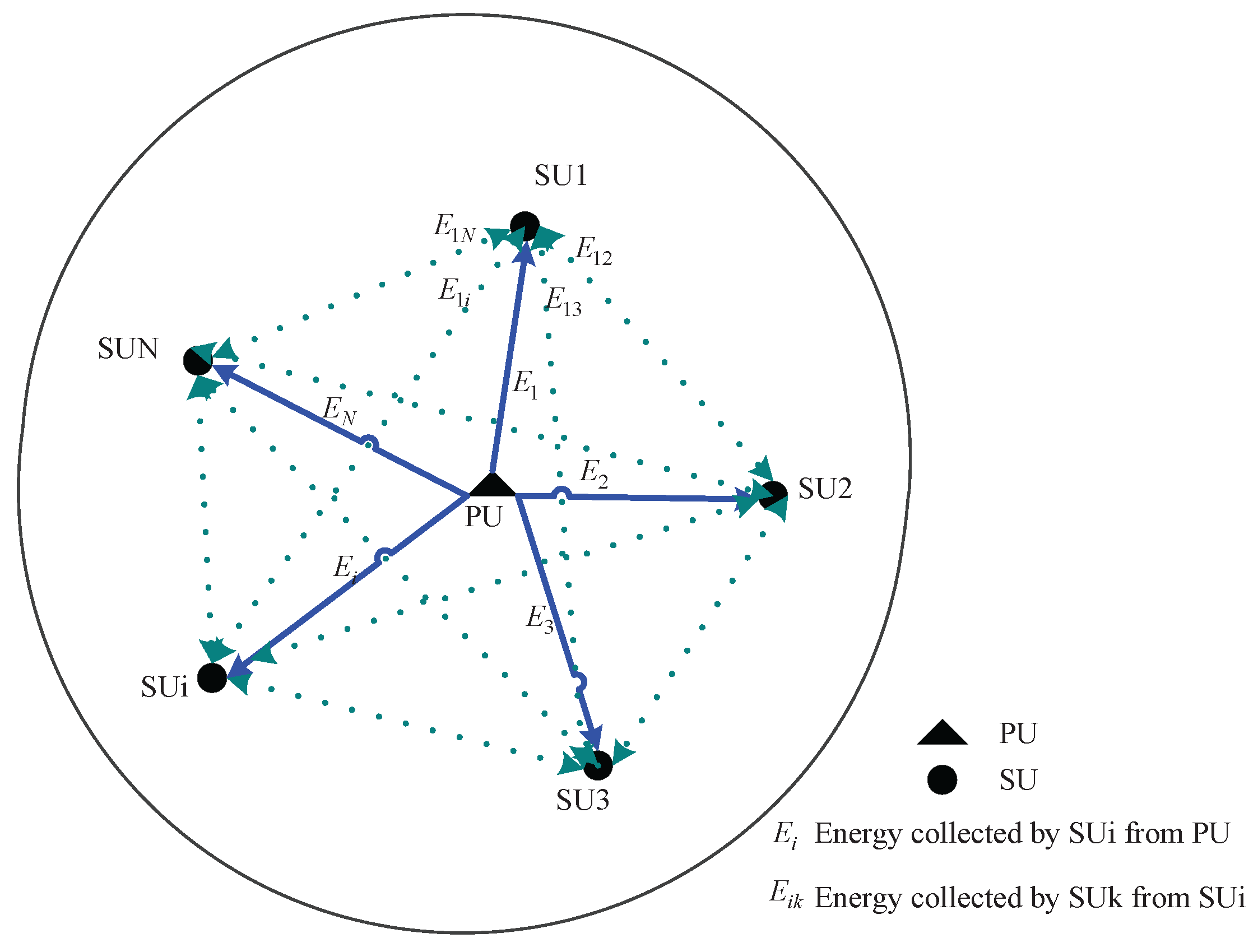
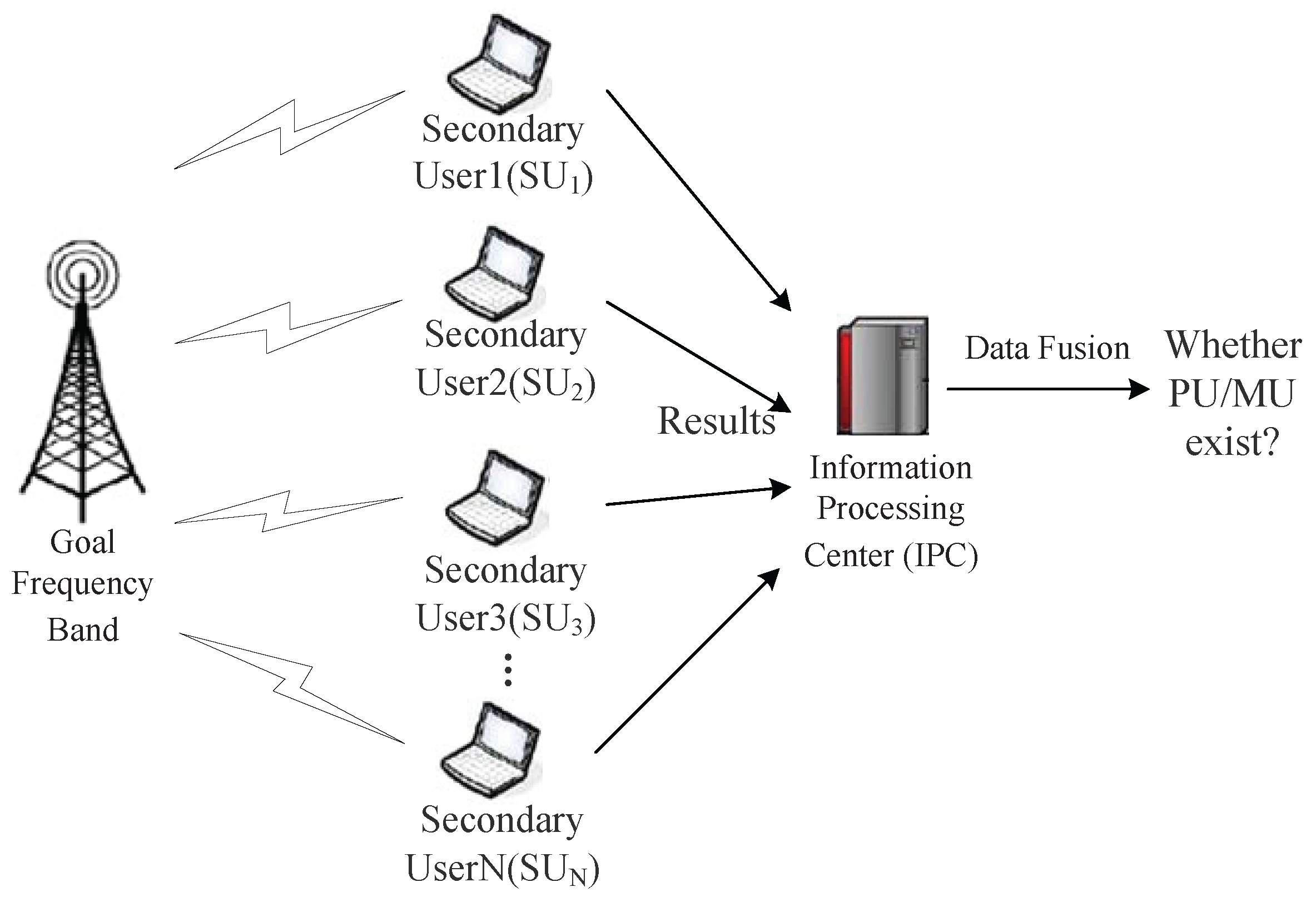
The data shown in Figure 2 assume that N SUs are randomly distributed in CRN. Based on the corresponding relation between received source signal energy and its location, the source signal collects received energy at each receiver, namely energy fingerprint, which is regarded as its exclusive identity label. Within one sensing period, SUs collect the energy of the source signal within the sensing band. We define $E_i$ as the energy collected at the $i_{th}$ SU from source signal node, where $i=1,2,\cdots ,N$, then the energy fingerprint of the source signal node can be described as:

$$\mathit{E}={(E_1,\cdots ,E_i,\cdots ,E_N)}^T$$

(9)

Similarly, we define $E_{ik}$ as energy from the $i_{th}$ SU to the $k_{th}$ SU (the theoretical energy value between two nodes can be calculated using the signal transmission model). Then energy fingerprints between the $i_{th}$ cognitive node and all SUs are defined as ${\mathit{m}}_i={(E_{i1},\cdots ,E_{ik},\cdots ,E_{iN})}^T$, where the value of $E_{ik}$ can be obtained using channel transmission model or actual measurement. In distributed cognitive radio networks, nodes that participate in the collaborative spectrum sensing can acquire sensing information of neighboring nodes by reporting channels (such as the energy values required by the algorithm in this paper). The channel transmission model or measured values are two kinds of means to obtain energy values. We use the channel transmission model to obtain the energy value and use the software platform to simulate the algorithm. When the algorithm is applied to the actual wireless scenarios, the measured energy values are indispensable.

All the energy fingerprints of SUs in CRN are combined into the sparse transforming matrix M:

$$\mathit{M}={({\mathit{m}}_1,\cdots ,{\mathit{m}}_i,\cdots ,{\mathit{m}}_N)}^T$$

(10)

Energy fingerprint $\mathit{E}$ can be represented according to sparse transforming basis $\mathit{M}$:

$$\mathit{E}=\sum _{i=1}^N{\mathit{m}}_i{\mu }_i=\mathit{M}\mathit{\mu }$$

(11)

where ${\mu }_i$ represents the degree of correlation between the $i_{th}$ SUs and source signal node, $\mathit{\mu }={({\mu }_1,\cdots ,{\mu }_i,\cdots ,{\mu }_N)}^T$. Generally, once SUs get closer to the source signal node, the signal energy fingerprint between it and other SUs becomes more similar. In other words, as the distance between SUs and the source signal node gets smaller, the degree of correlation ${\mu }_i$ becomes greater, otherwise ${\mu }_i$ will be smaller or even zero. Furthermore, the main constituents of energy fingerprint $\mathit{E}$ are described by a few close SUs’ energy fingerprints. Only several SUs has greater correlation coefficients, and the rest are zero or close to zero. It means that the degree of correlation vector μ is sparse.

According to Equation (4), defining CS information operator as ${\mathit{A}}^{{}^{\prime }}=\mathit{\Psi }\mathit{M}$ , thus measurement vector $\mathit{y}$ can be written as

$$\mathit{y}=\mathit{\Phi }\mathit{E}=\mathit{\Phi }\mathit{M}\mathit{\mu }={\mathit{A}}^{{}^{\prime }}\mathit{\mu }$$

(12)

where y is the measurement vector of each SU received signal strength (RSS), $\mathit{\Phi }$ is grid transfer relationship between each SU and PU source signal. The normalized correlation coefficient μ can be reconstructed by basic CS according to Equation (6).

Then the weighted value ${\omega }_i$ of each SU can be obtained as follows

$${\omega }_i=\frac{{\mu }_i}{{\sum }_{i=1}^N{\mu }_i}$$

(13)

Assume $(S_i\left(x\right),S_i\left(y\right))$ is coordinate of the $i_{th}$ SU, then 2-dimensional location of source signal node $\left(P\right(x),P(y\left)\right)$ can be estimated by using WCL

$$(P\left(x\right),P\left(y\right))=\sum _{i=1}^N{\omega }_i(S_i\left(x\right),S_i\left(y\right))$$

(14)

The following Figure 3 denotes the source node localization flowchart of the PU-CSL algorithm during one sensing period.

In fact, the correlation degree increases as nodes become closer to each other. However, there is also one point that needs to be clear: the proposed PU-CSL algorithm that integrally explores the correlation between source signal and SUs using CS. The correlation between source signal and SUs is the decisive factor to determine the result of the positioning. Hence we put the main focus on how to integrally explore the correlation between source signal and SUs and achieve higher localization accuracy.

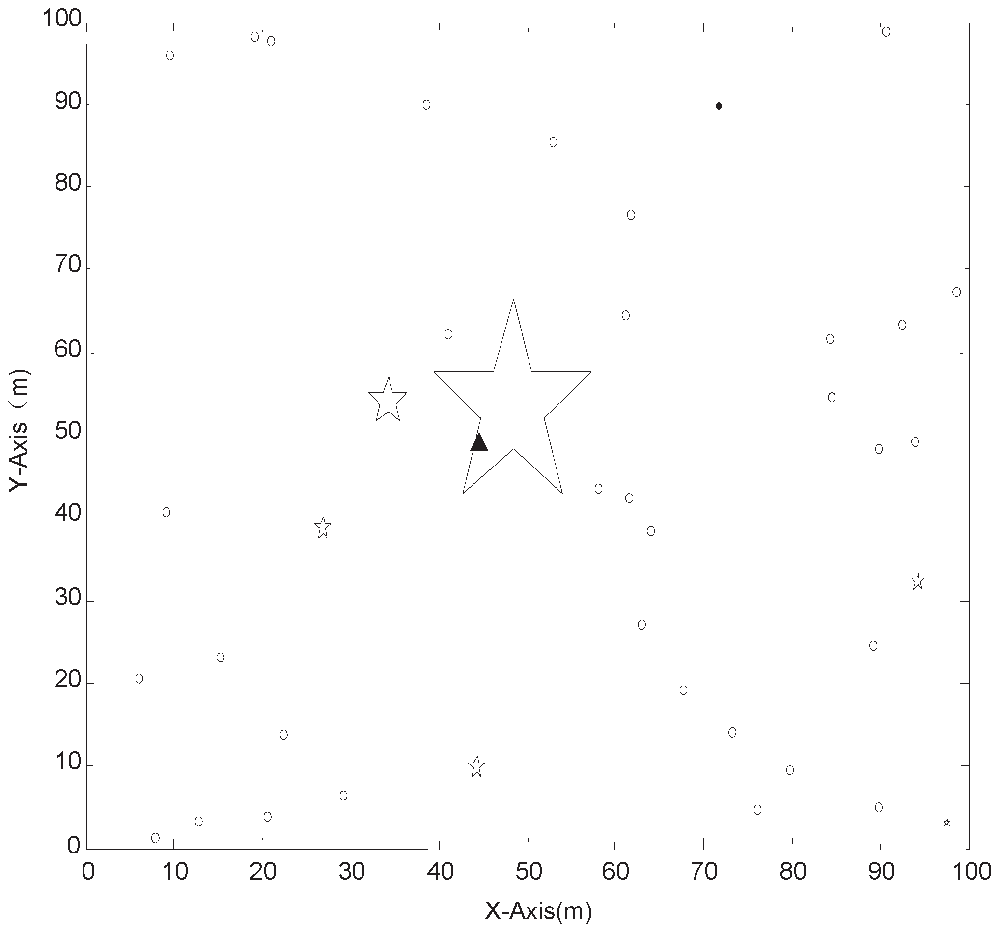
Figure 4 describes how the source node is linearly represented by 40 SUs which are randomly distributed in a quadrate sensing area of 100 × 100 m². The black solid triangles in the figure are the source node, the circles and five-pointed star show the SUs, the circle represents a SU whose correlation coefficient is zero, and the five-pointed star denotes the the SUs whose correlation coefficient is nonzero. There is positive correlation between the size of pentagram and the correlation coefficient of the node.

As can be seen from Figure 4, the greater the correlation coefficient of the node is, the closer the geometric position are to the source node. The SU with relatively small and even zero correlation coefficient is always far away from the source node.

More importantly, in the sensing area, few SUs have a large correlation coefficient. Most of the nodes’ correlation coefficients are zero or close to zero, that is, the vector that constitutes of all the correlation coefficient of SUs is sparse. The conclusion is consistent with the above theoretical analysis. Therefore, the degree of correlation between SUs and source node can be accurately reconstructed using CS theory, thus it is possible to estimate the location of the source node.

5. Simulation and Analysis of Localization Performance

The localization performance of the proposed PU-CSL scheme has been simulated and compared with RR-WCL scheme using MATLAB ( [13] has proved that the localization performance of RR-WCL is much better than W-Centroid, RR-WCL is then chosen as comparison). Here is the simulation environment. There is one source signal node, $N=40$. SUs are randomly distributed in a quadrate sensing localization area of $100\mathrm{m}\times 100\mathrm{m}$. The parameters of the signal model are respectively set as $P_t=40\mathrm{dBm}$, $\eta =2$, $d_0=1\mathrm{m}$. After balancing spectrum efficiency and observation times, the death rate α and birth rate β in the PU activity model [17] are both set as 1. The mean and standard deviation value of shadow fading factor $X_{\sigma }$ are respectively 0 and 4. The energy fingerprints of nodes are obtained based on signal loss model Equation (2), the correlation coefficients are reconstructed by CS using BP algorithm.

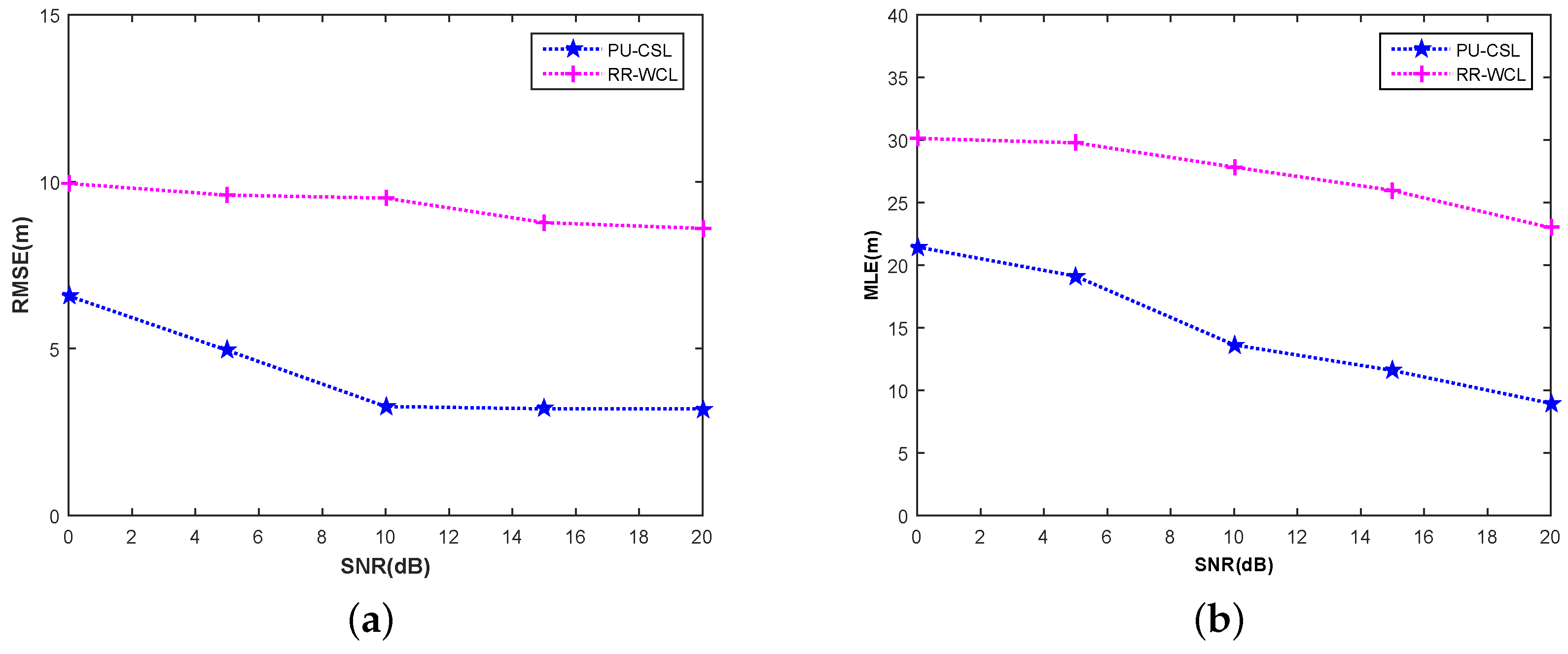
Figure 5 displays the comparative result of PU-CSL and RR-WCL concerning the root mean square error of location error (we recall the definition of root mean square error as RMSE = $\parallel X-\widehat{X}\parallel$, where X is the original observation and $\widehat{X}$ is the reconstructed signal) and MLE (the maximum location error is the maximum distance between the actual position and the predicted position of the node). The signal-to-noise ratio (SNR) is 0 dB∼20 dB and the amount of SUs N in spectrum sensing is 40.

Several points can be found from the curves. Firstly, the root mean square error and maximum location error of both algorithms continually decrease as $\mathrm{SNR}$ increases. This is because the energy fingerprints of the SUs and the source signal node become more similar when $\mathrm{SNR}$ is lower, which leads to better localization performance. Secondly, as $\mathrm{SNR}$ changed between $0\mathrm{dB}$ and $20\mathrm{dB}$ , the root mean square error and maximum location error of the PU-CSL respectively improved by 33.38%∼65.66% and 28.20%∼71.04% compared to the PR-WCL, which means that PU-CSL exhibits better anti-noise performance. Besides, under the condition of same $\mathrm{SNR}$, both of the root mean square error and maximum location error of PU-CSL are smaller than RR-WCL. Therefore, PU-CSL shows higher localization accuracy. Since RR-WCL merely concerns the degree of correlation between nodes and the source node, the proposed PU-CSL algorithm integrally explores the correlation between source signal and SUs using CS. Hence, the source signal node is preferably described by SUs with correlation property. However, PU-CSL achieves higher localization accuracy.

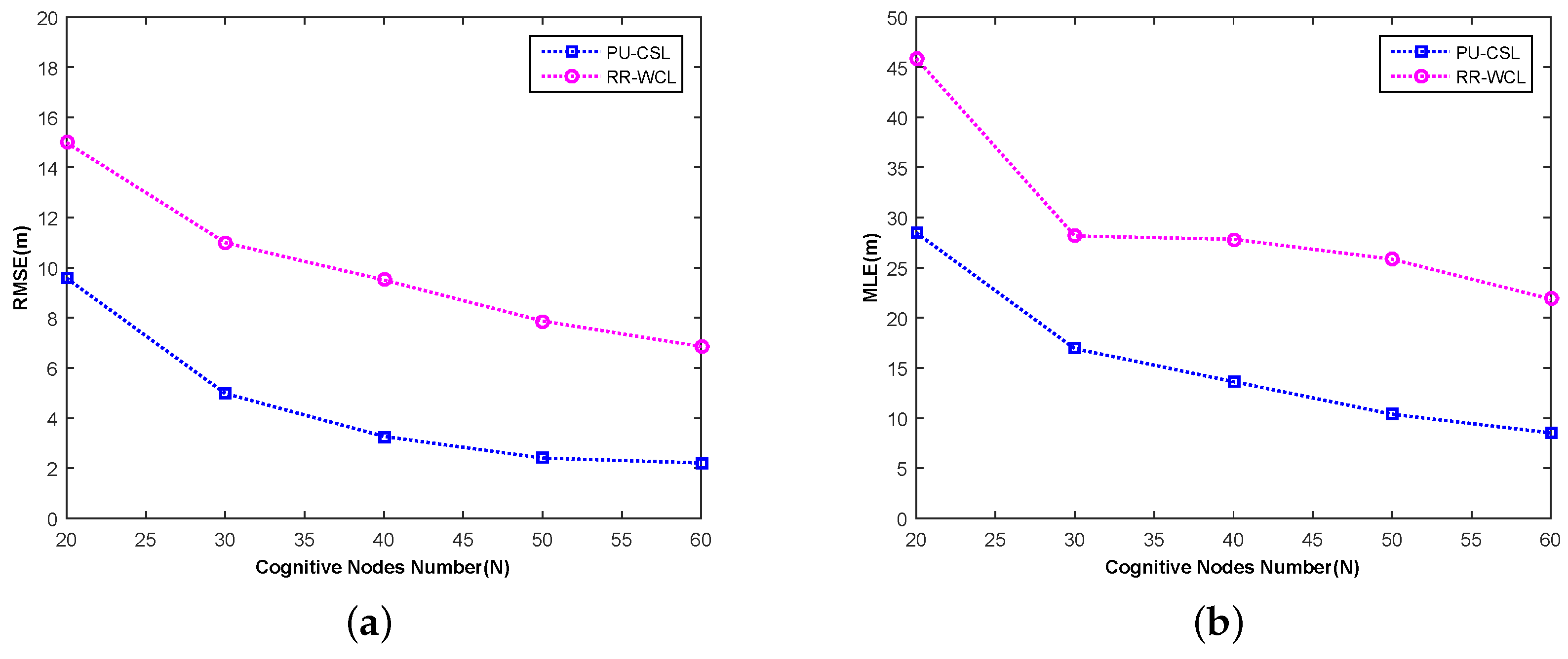
Figure 6 shows the localization performance with respect to the change of root mean square error and maximum location error as the number of SUs N changes, where $\mathrm{SNR}=10\mathrm{dB}$.

There are two aspects that can be inferred from Figure 6. Firstly, the root mean square error and maximum location error of both algorithms decrease with the increase of the amount of SUs. In other words, the more nodes getting involved in CSS, the higher localization accuracy of the source signal node is obtained. However, in actual CRN, as the number of SUs increases, the information sent to IPC also increases and request for ${\mathrm{IPC}}^{{}^{\prime }}$ data processing ability gets higher. Thus, in practice, we should choose a suitable number of cognitive nodes for the localization of source signal node, comprehensively considering the hardware cost and localization performance of the network in the meantime. Secondly, as the number of SUs changes between 20 and 60, the root mean square error and maximum location error of the PU-CSL algorithm respectively improved by 36.10%∼69.46% and 37.92%∼61.08% compared to the PR-WCL, which means that the PU-CSL exhibits better localization performance. Besides, with the same number of cognitive nodes, the PU-CSL outperforms the RR-WCL in localization performance. Being different from RR-WCL, PU-SCL explores the degree of correlation between source signal and SUs integrally at one time using CS. Therefore, it performs higher localization accuracy due to making more comprehensive consideration of the source localization.

6. Conclusions

The localization for source signal plays a significant role in resisting PUEA in CRN. This paper put forward a brand new primary user localization algorithm based on compressive sensing in cognitive radio networks (PU-CSL). PU-CSL considers received source signal strength as source fingerprints, using compression sensing to obtain correlation between SUs and source signal, constructing weighted coefficients of SUs based on the relevant information, and, finally, estimating source location by the weighted centroid algorithm. Experimental results show that the proposed PU-CSL scheme outperforms the RR-WCL scheme on localization and anti-noise performance. As PU-CSL integrally explores the geographical correlation between source signal and SUs using CS, the source signal is preferably described by SUs and the localization of the source node becomes more accurate.