1. Introduction
Big data describe data sets that grow so large that they become unpractical to be processed by traditional tools like database management systems, content management systems, advanced statistical analysis software, and so forth. The reason why they came into the attention of the research community is that the infrastructure to handle these data sets has become more affordable due to
Cloud Computing and
MapReduce [
1] based open-source frameworks. The vision of everyday people inspecting large amounts of data, easily interacting with graphical interfaces of software applications that handle
data mining tasks, has indeed enthused final users. On the other hand, those tools have to leverage people’s ability to answer analytical processes by inference through large amounts of data.
The problem with this data is not the complexity of the processes involved, but rather the quantity of data and the rate of collecting new data. The following two examples are slightly illustrative of this phenomenon.
In April 2009,
EBay was using two Data Warehouses, namely
Teradata and
Greenplum, the former having 6.5 PB of data in form of 17 trillion records already stored, and collecting more than 150 billion new records/day, leading to an ingest rate well over 50 TB/day [
2].
In May 2009,
Facebook estimates an amount of 2.5 PB of user data, with more than 15 TB of new data per day [
3].
As another matter of question, the presence of
graph-based data structures occurs almost everywhere starting with
social networks like
Facebook [
4],
MySpace [
5] and
NetFlix [
6], and ending with
transportation routes or
Internet infrastructure architectures. These graphs keep growing in size and there are several new things that people would like to infer from the many facets of information stored in these data structures. Graphs can have billions of vertices and edges. Citation graphs, affiliation graphs, instant messenger graphs, phone call graphs and so forth, are part of the so-called
social network analysis and mining initiative. Some recent works show that, despite the previously supposed sparse nature of those graphs, their density increases over time [
7,
8]. All considering, these trends tend towards the so-called
big Web data (e.g., [
9,
10]), the transposition of big data on the Web.
On the other hand,
Semantic Web technologies allow us to effectively support analysis of large-scale distributed data sets by means of the well-known
Resource Description Framework (RDF) model [
11], which, obviously represents data via a
graph-shaped approach. As a consequence, in the Semantic Web initiative, the most prominent kind of graph data are represented by
RDF graphs. This opens the door to a wide family of database-like applications, such as
keyword search over RDF data (e.g., [
12]).
While RDF graphs offer a meaningful data model for successfully representing, analyzing and mining large-scale graph data, the problem of
efficiently processing RDF graphs is still an open issue in database research (e.g., [
13,
14,
15]). Following this main consideration, in this paper, we focus on
the problem of computing traversals of RDF graphs, being computing traversals of such graphs very relevant in this area, e.g., for RDF graph analysis and mining over large-scale data sets. Our approach adopts the
Breadth First Search (BFS) strategy for visiting (RDF) graphs to be decomposed and processed according to the MapReduce framework. This with the goal of taking advantages from the powerful run-time support offered by MapReduce, hence reducing the computational overheads due to manage large RDF graphs efficiently. This approach is conceptually-sound, as similar initiatives have been adopted in the vest of viable solutions to
the problem of managing large-scale sensor-network data over distributed environments (e.g., [
16,
17]), like for the case of Cloud infrastructures and their integration with sensor networks. We also provide experimental results that clearly confirm the benefits coming from the proposed approach.
The remaining part of this paper is organized as follows. In
Section 2, we provide an overview of
Hadoop [
18], the software platform that incorporates MapReduce for supporting complex
e-science applications over large-scale distributed repositories.
Section 3 describes in more details principles and paradigms of MapReduce. In
Section 4, we provide definitions, concepts and examples on RDF graphs.
Section 5 contains an overview on state-of-the-art approaches that represent the knowledge basis of our research. In
Section 6, we provide our efficient algorithms for implementing BFS-based traversals of RDF graphs over MapReduce.
Section 7 contains the result of our experimental campaign according to which we assessed our proposed algorithm. Finally, in
Section 8, we provide conclusions of our research and depict possible future work in this scientific field.
2. Hadoop: An Overview
Hadoop is an open-source project from
Apache Software Foundation. Its core consists of the MapReduce programming model implementation. This platform was created for solving the problem of processing very large amounts of data, a mixture of complex and structured data. It is used with predilection in the situation where data-analytics-based applications require a large number of computations have to be executed. Similar motivations can be found in related research efforts focused on the issue of effectively and efficiently managing large-scale data sets over
Grid environments (e.g., [
19,
20,
21]).
The key characteristic of Hadoop is represented by the property of enabling the execution of applications on thousands of nodes and peta-bytes of data. A typical enterprise configuration is composed by tens or thousands of physical or virtual machines interconnected through a fast network. The machines run a POSIX compliant operating system and a Java virtual machine.
Cutting was the creator of the Hadoop framework, and two papers published by Google’s researchers had decisive influence on his work:
The Google File System [
22] and
MapReduce: Simplified Data Processing on Large Clusters [
1]. In 2005, he started to use an implementation of MapReduce in
Nutch [
23], an application software for web searching, and very soon the project becomes independent from
Nutch under the codename
Hadoop, with the aim of offering a framework for running many jobs within a cluster.
The language used for the development of the Hadoop framework was Java. The framework is providing the users with a Java API for developing MapReduce applications. In this way, Hadoop becomes very popular in the community of scientists whose name is linked to the big data processing.
Yahoo! is an important player in this domain, this company having for a longer period a major role in the design and implementation of the framework. Another big player is Amazon [
24], company currently offering a web service [
25] based on Hadoop that is using the infrastructure provided by the
Elastic Compute Cloud—EC2 [
26]. Meanwhile, Hadoop becomes very highly-popular, and, in order to sustain this allegation, it is sufficient just to mention the presence of other important players like
IBM,
Facebook,
The New York Times,
Netflix [
27] and
Hulu [
28] in the list of companies deploying Hadoop-based applications.
The Hadoop framework hides the details of processing jobs, leaving the developers liberty to concentrate on the application logic. The framework has the following characteristic features:
- (1)
accessible—it can be executed on large clusters or on Cloud computing services;
- (2)
robust—it was designed to run on commodity hardware; a major aspect considered during its development was the tolerance to frequent hardware failures and crash recovery;
- (3)
scalable—it scales easily for processing increased amount of data by transparently adding more nodes to the cluster;
- (4)
simple—it allows developers to write specific code in a short time.
There is quite a large application domain for Hadoop. Some examples include online e-commerce applications for providing better recommendations to clients looking after certain products, or finance applications for risk analysis and evaluation with sophisticated computational models whose results cannot be stored in a database.
Basically, Hadoop can be executed on each major OS: Linux, Unix, Windows, Mac OS. The platform officially supported for production is Linux only.
The framework is implementing a master-slave architecture used both for distributed data storage and for distributed computing. Hadoop framework running on a completely-configured cluster is composed of a set of daemons or internal modules executed on various machines of the cluster. These daemons have specific tasks, some of them running only on a single machine, others having instances running on several machines.
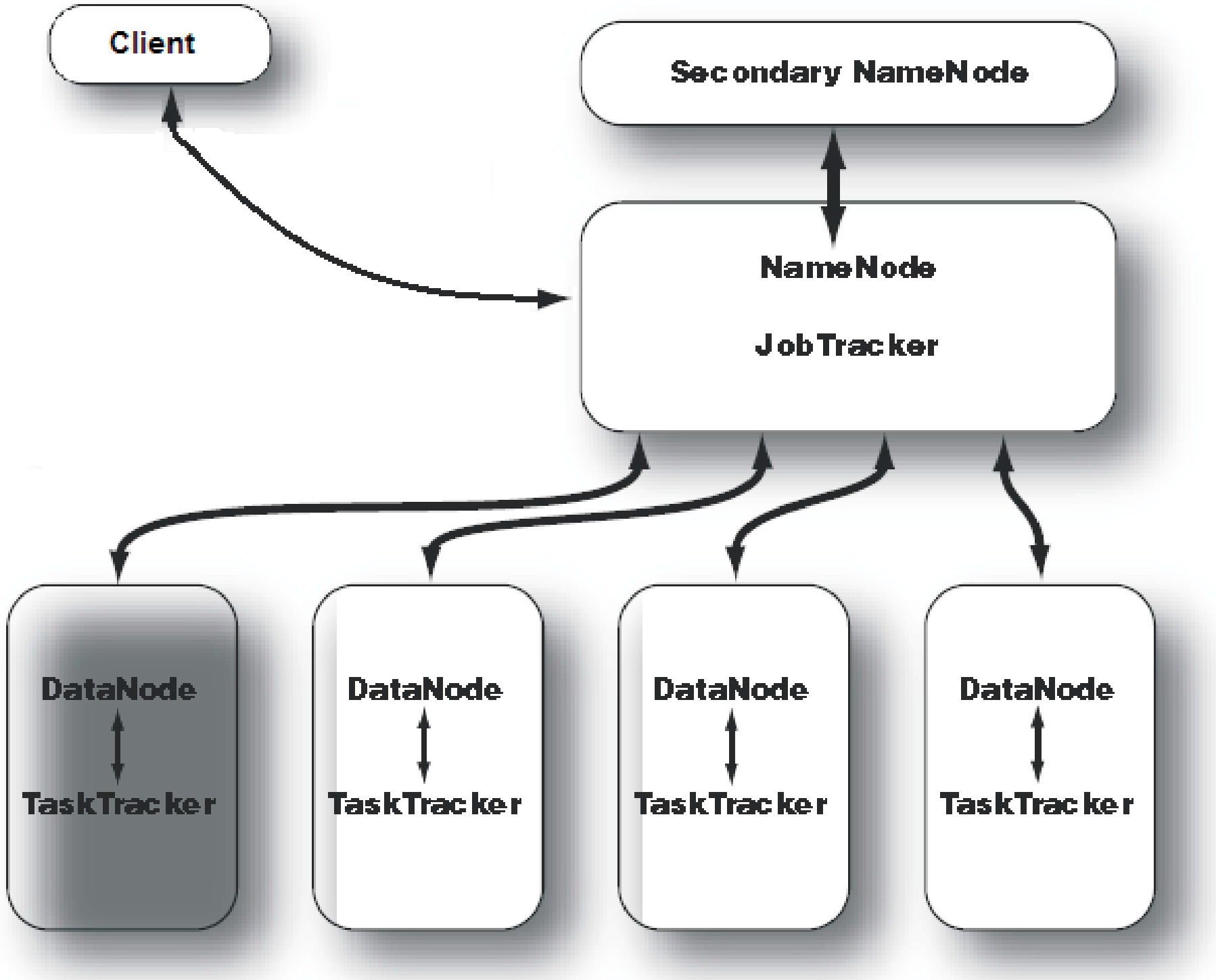
A sample Hadoop cluster architecture is depicted in
Figure 1. For a small cluster,
Secondary NameNode daemon can be hosted on a slave node, meanwhile, on a large cluster, it is customary to separate the
NameNode and
JobTracker daemons on different machines. In
Figure 1, a master node is running
NameNode and
JobTracker daemons and an independent node is hosting the
Secondary NameNode daemon, just in case of failure in the master node. Each slave machine hosts two daemons,
DataNode and
TaskTracker, in order to run computational tasks on the same node where input data are stored.
Figure 1.
Hadoop cluster architecture.
Figure 1.
Hadoop cluster architecture.
As regards the proper data storage solution, Hadoop’s ecosystem incorporates
HBase [
29]. HBase is a
distributed column-oriented database (e.g., [
30]), which also falls in the category of
NoSQL storage systems (e.g., [
31]), that founds on the underlying
Hadoop Distributed File System (HDFS) (e.g., [
32]) for common data processing routines. HBase has been proved to be highly scalable. HBase makes use of a specific model that is similar to
Google’s BigTable (e.g., [
33]), and it is designed to provide fast random access to huge amounts of structured data. As regards the main software architecture organization, HBase performs read/write (fast) routines on HDFS while data consumer and data producer applications interact with (big) data through HBase directly. Recently, due to its relevance, several studies have focused on HBase.
3. MapReduce: Principles of Distributed Programming over Large-Scale Data Repositories
MapReduce is both a programming model for expressing distributed computations on massive amounts of data and an execution framework for large-scale data processing on clusters of commodity servers [
1,
34]. MapReduce’s programming model was released to the computer science community in 2004, being described in [
1] after Google was already using this technology for a couple of years. MapReduce’s processing scheme soon became very popular, including a broad adoption due to its open-source implementation. A job from MapReduce programming model splits the input data set into several independent blocks that are processed in parallel.
There are two seminal ideas that are encountered in MapReduce, which we report in the following.
There is a previous well-known strategy in computer science for solving problems: divide-et-impera. According to this paradigm, when we have to solve a problem whose general solution is unknown, then the problem is decomposed in smaller sub-problems, the same strategy is applied for it, and the results/partial solutions corresponding to each sub-problem into a general solution are combined. The decomposing process continues until the size of the sub-problem is small enough to be handled individually.
The basic data structures are key-value pairs and lists. The design of MapReduce algorithms involves usage of key-value pairs over arbitrary data sets.
Map and Reduce concepts were inspired from functional programming. Lisp, in particular, introduces two functions with similar meaning, map and fold. Functional operations have the property of preserving data structures such that the original data remains unmodified and new data structures are created. The map function takes as arguments a function f and a list, and it applies the function f to each element of the input list, resulting in a new output list. The fold function has an extra argument compared to the map: beyond the function f and the input list, there is an accumulator. The function f is applied to each element of the input list, the result is added to previous accumulator, thus obtaining the accumulator value for the next step.
Although the idea seems to be very simple, implementation details of a
divide-and-conquer approach are not. There are several aspects with which practitioners must deal. Some are the following ones:
decomposition of the problem and allocation of sub-problems to workers;
synchronization among workers;
communication of the partial results and their merge for computing local solutions;
management of software/hardware failures;
management of workers’ failures.
The MapReduce framework hides the peculiarities of these details, thus allowing developers to concentrate on the main aspects for implementation of target algorithms.
Technically-wise, for each job, the programmer has to work with the following functions:
mapper,
reducer,
partitioner and
combiner. The
mapper and
reducer have the following signatures:
where […] denotes a list.
The input of a MapReduce’s job is fetched from the data stored in the target distributed file system. For each task of type map, a mapper is created. This is a method which, applied to each input key-value pair, returns a number of intermediary key-value pairs. The reducer is another method applied to a list of values associated with the same intermediary key in order to obtain a list of key-value pairs. Transparently to the programmer, the framework implicitly groups the values associated with intermediary keys between the mapper and the reducer.
The intermediary data reach the
reducer ordered by key, and there is no guarantee regarding the key order among different reducers. The
key-value pairs from each
reducer are stored in the distributed file system. The output values from each
reducer are stored also in
m files from the distributed file system, considered these latter as output files for each
reducer. Finally, the
map() and
reduce() functions run in parallel, such that the first
reduce() call cannot start before the last
map() function ends. This is an important separation point among different phases. Simplifying, at least the MapReduce developer has to implement interfaces of the two following functions:
hence allowing her/him to concentrate on the application logic while discarding the details of a high-performance, complex computational framework.
In the context of data processing and query optimization issues for MapReduce,
Bloom filters [
35] and
Snappy data compression [
36] play a leading role as they are very often used to further improve the efficiency of MapReduce. Indeed, they are not only conceptually-related to MapReduce but also very relevant for our research, as they are finally integrated in our implemented framework (see
Section 6). Bloom filters are
space-efficient probabilistic data structures initially thought to test whether an element is member of a set or not. Bloom filters have a 100%
recall rate, since false positive matches are possible, whereas false negative matches are not possible. It has been demonstrated that Bloom filters are very useful tools within MapReduce tasks, since, given the fact that they avoid false negatives, they allow for getting rid of irrelevant records during
map phases of MapReduce tasks, hence configuring themselves as a very reliable space-efficient solution for MapReduce. Snappy data compression is a
fast C++ data compression and decompression library proposed by
Google. It does not aim at maximizing compression, but, rather, it aims at achieving a very high compression speed at a reasonable compression ratio. Given its orthogonality, Snappy has been used not only with MapReduce but also in other Google projects like BigTable.
4. RDF Graphs: Definitions, Concepts, Examples
Since RDF graphs play a central role in our research, in this Section, we focus in a greater detail on definitions, concepts and algorithms of such very important data structures of the popular Semantic Web. RDF is a Semantic Web data model oriented to represent
information on resources available on the Web. To this end, a critical point is represented by the fact that RDF model
metadata about such Web resources, which can be defined as data that describe other data. Thanks to metadata, RDF can easily implements some very important functionalities over the Semantic Web, such as: resource representation, querying resource on the Web, discovering resources on the Web, resource indexing, resource integration, interoperability among resources and applications, and so forth. RDF is primarily meant for managing resources on the Web for applications, not for end-users, as to support
querying the Semantic Web (e.g., [
37]),
Semantic Web interoperability (e.g., [
38]),
complex applications (e.g., [
39]), and so forth.
Looking into more details, RDF is founded on the main assertion that resources are identified on the Web via suitable
Web identifiers like
Uniform Resource Identifiers (URI) and they are described in terms of
property-value pairs via
statements that specify these properties and values. In an RDF statement, the
subject identifies the resource (to be described), the
predicate models the property of the subject, and the
object reports the value of that property. Therefore, each RDF resource on the Web is modeled in terms of the triple (
subject,
predicate,
object). This way, since Web resources are typically connected among them, the Semantic Web represented via RDF easily generates the so-called RDF graphs. In such graphs, RDF models statements describing Web resources via nodes and arcs. In particular, in this graph-ware model, a statement is represented by: (
i) a node for the subject; (
ii) a node for the object; (
iii) an arc for the predicate, which is directed from the node modeling the subject to the node modeling the object. In terms of the popular
relational model, an RDF statement can be represented like a tuple (
subject,
predicate,
object) and, as a consequence, an RDF graph can be naturally represented via a
relational schema storing information on subjects, predicated and objects of the corresponding Web resources described by the RDF statements modeled by that graph (e.g., [
40]).
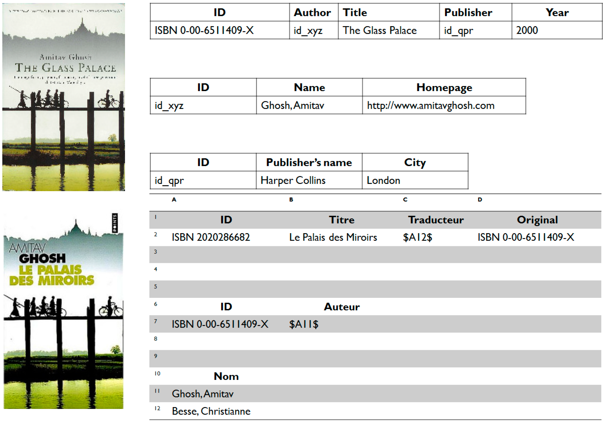
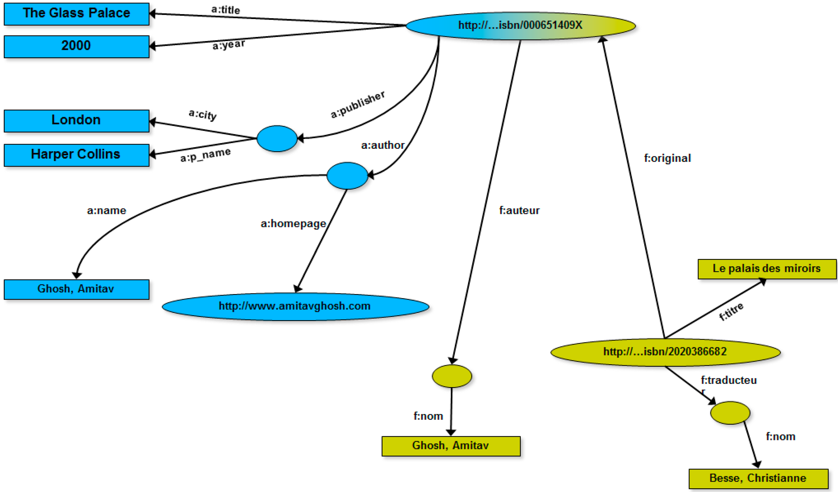
Figure 2.
Different Web media for the same book (
left); and their corresponding relational schemas (
right) [
41].
Figure 2.
Different Web media for the same book (
left); and their corresponding relational schemas (
right) [
41].
Figure 2, borrowed from [
41], shows an example where information on the Web regarding the book “
The Glass Palace”, by A. Ghosh, occurs in two different sites in the vest of different media, one about the English version of the book, and the other one about the French version of the book. According to this, the two different Web resources are represented by two different relational schemas (see
Figure 2).
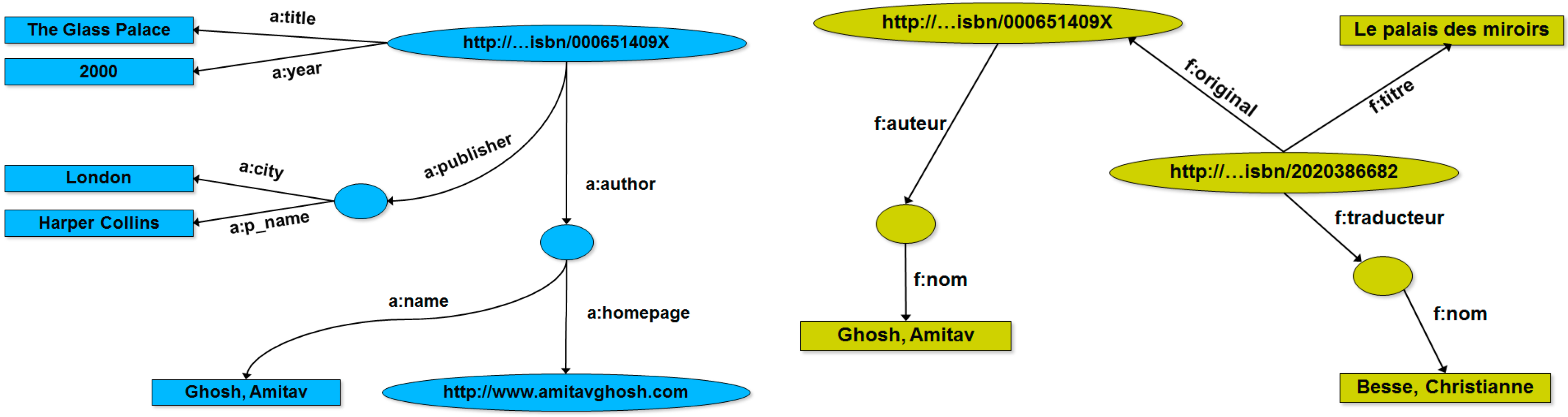
Figure 3, instead, shows the corresponding RDF graphs for the two different Web resources, respectively.
Figure 3.
The two RDF graphs corresponding to the two different Web media for the same book reported in
Figure 2 [
41].
Figure 3.
The two RDF graphs corresponding to the two different Web media for the same book reported in
Figure 2 [
41].
As highlighted before, one of the goals of RDF graphs is allowing the easy integration of correlated Web resources. This is, indeed, a typical case of Web resource integration because the two RDF graphs, even if different, describe two different media of the same resource. It is natural, as a consequence, to integrate the two RDF graphs in a unique (RDF) graph, even taking advantage from the “natural” topological nature of graphs, as shown in
Figure 4. In particular, the integration process is driven by recognizing the same URI that identifies the book resource.
Figure 4.
RDF graph obtained via integrating the two RDF graphs of
Figure 3 [
41].
Figure 4.
RDF graph obtained via integrating the two RDF graphs of
Figure 3 [
41].
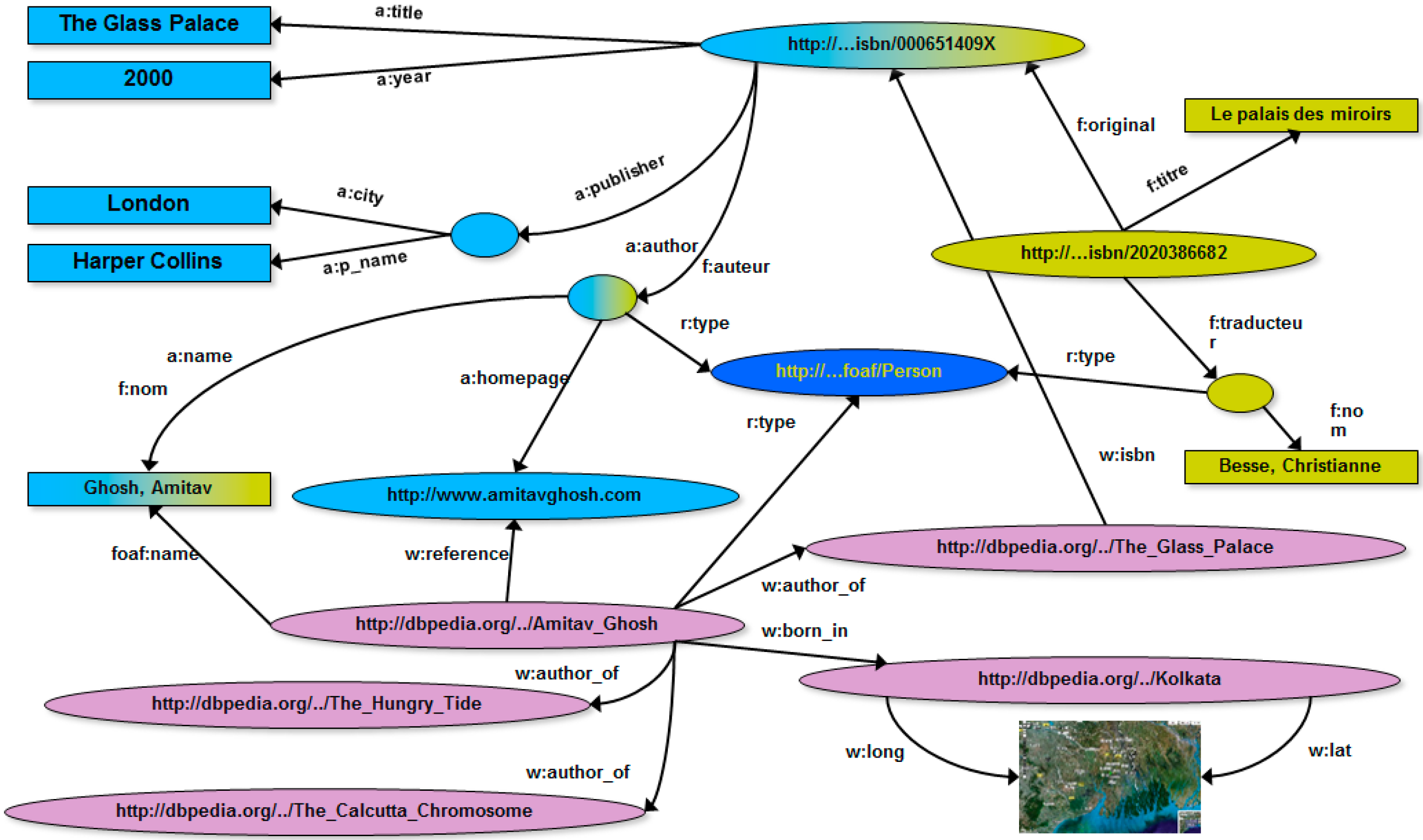
Another nice property of the RDF graph data model that makes it particularly suitable to Semantic Web is its “open” nature, meaning that any RDF graph can be easily integrated with
external knowledge on the Web about resources identified by the URIs it models. For instance, a common practice is that of integrating RDF graph with Web knowledge represented by
Wikipedia [
42] via ad-hoc tools (e.g.,
DBpedia [
43]). This contributes to move the actual Web towards the Web of data and knowledge.
Figure 5 shows the RDF graph of
Figure 4 integrated with knowledge extracted from Wikipedia via DBpedia.
Figure 5.
RDF graph obtained via integrating the RDF graph of
Figure 4 with Wikipedia knowledge extracted via DBpedia [
41].
Figure 5.
RDF graph obtained via integrating the RDF graph of
Figure 4 with Wikipedia knowledge extracted via DBpedia [
41].
It is worth noticing that, when RDF graphs are processed, applications can easily extract knowledge from them via so-called
RDF query language [
44] or other AI-inspired approaches (e.g., [
45]). In addition to this, computing traversal paths over such graphs is critical for a wide range of Web applications. To give an example, traversal paths can be used as “basic” procedures of powerful
analytics over Web Big Data (e.g., [
46]). This further gives solid motivation to our research.
6. BFS-Based Implementation of RDF Graph Traversals over MapReduce
There exist in literature two well-known approaches for representing a graph: through an
adjacency matrix, and through
adjacency lists. The former has the advantage of
constant lookup over graph data, with the drawback of an increased usage of memory (
, where
represents the number of vertices), also for sparse graphs. In practice, while the majority of graphs are not so dense, we end with a waste of space having a big matrix with few values (not all the cells of the matrix will be used to store a value). The latter stores, for every vertex, a list of vertices connected to it (called
adjacent nodes), thus reducing the overall memory requirement. This representation has also the advantage of being suited to feed a MapReduce job. As regards the proper RDF graph implementation as
Abstract Data Type (ADT), we exploited the well-known
Apache Jena RDF API [
74], which models the target RDF graph in terms of collection of
RDF nodes, which are connected via a
direct graph by means of
labelled relations.
There are several algorithms for visiting a graph, but BFS (see Algorithm 1) has been proven to be more suited for parallel processing. BFS algorithm cannot be expressed into a single MapReduce job directly, because the while construct at every step increments the frontier of exploration in the graph. Moreover, this frontier expansion permits the finding of the paths to every node explored from the source node. Since the BFS algorithm cannot be codified within a MapReduce job, we propose a novel approach to coordinate a series of MapReduce jobs that check when to stop the execution of these jobs. This is called convergence criterion. To this end, we propose feeding the output of a job as the input of the successive one, and to apply a way to count if further nodes must be explored via maintaining a global counter updated at each iteration that, in the standard BFS, is represented by the iterator’s position in the queue itself. In our proposed implementation, the only convergence criterion that we make use of is thus represented by counting the jobs that terminate (to this end, MapReduce’s DistributedCache is exploited), but of course other more complex criteria may be adopted in future research efforts (e.g., based on load balancing issues).
| Algorithm 1: BFS(u, n, L) |
Input: u – source node from which the visit starts; n – number of vertices; L – adjacency lists
Output: Q – list of visited nodes

Begin
  Q ← ∅;
  visited ← ∅;
  for (i = 0 to n – 1) do
    visited[i] = 0;
  endfor;
  visited[u] = 1;
  Q ← u;
  while (Q ≠ ∅) do
    u ← Q;
    for (each v ∈ Lu) do     // Lu is the adjacency list of u
      if (visited[v] == 0) then
        visited[v] = 1;
        Q ← v;
      endif;
    endfor;
  endwhile;
  return Q;
End;
|
Basically, in order to control the algorithmic flow and safely achieve the convergence criterion, the proposed algorithm adopts the well-known
colorability programming metaphor. According to this programming paradigm, graph processing algorithms can be implemented by assigning a color-code to each possible node’s state (in the
proper semantics of the target algorithm) and then superimposing certain actions for each specific node’s state. This paradigm is, essentially, an enriched
visiting strategy over graphs, and, in fact, BFS is only a possible instance of such strategy. To this end, the proposed approach makes use of suitable
metadata information (stored into text files), which models, for each node of the graph stored in a certain Cloud node, its adjacent list plus additional information about the node’s state. An example of these metadata is as follows:
1 3,2, | GREY | 1
10 12, | WHITE | ?
11 10, | WHITE | ?
12 NULL, | WHITE | ?
13 NULL, | WHITE | ?
14 6,12, | WHITE | ?
In more detail, for each row, stored metadata have the following semantics: (see the previous example—the description is field-based): (i) the first number is the node ID; (ii) the subsequent list of numbers represents the adjacent list for that node, and it is equal to NULL if empty; (iii) the subsequent color-code represents the state of the node; (iv) the last symbol states if the target node has been processed (i.e., then, it is equal to “1”) or not (i.e., then, it is equal to “?”). The adoption of this metadata information exposes the clear advantage of supporting portability and interoperability within Cloud environments widely.
Looking into code-wise details, the proposed algorithm consists of a series of iterations where each iteration represents a MapReduce job using the output from the previous MapReduce job until the convergence criterion is met. The Mapper job (see Algorithm 2) allows us to expand the frontier of exploration by selecting the new nodes to explore (the ones that in the standard BFS algorithm are inserted into the queue) and the ones already explored (or still not explored), as to complete the output.
| Algorithm 2: Map(key, value) |
Input: key – ID of the current node; value – node information
Output: void – a new node is emitted

Begin
  u ← (Node)value;
  if (u.color == GREY) then
    for (each v ∈ Lu) do     // Lu is the adjacency list of u
      v ← new Node();
      v.color == GREY;   // mark v as unexplored
      for (each c ∈ Pu) do     // Pu is the path list of u
        c.ID = u.ID;
        c.tag = u.tag;
        v.add(c);
      endfor;
      emit(v.ID,v);
    endfor;
    u.color = BLACK;     // mark u as explored
  endif;
  emit(key,u);
  return;
End;
|
The Reducer job (see Algorithm 3) allows us to (i) merge the data provided by the Mapper and re-create an adjacency list that will be used at the next step and (ii) update the counter for the convergence test. More in detail, in order to merge nodes with the same ID, a color priority method was devised so that, in the case of the generation of a node with the same ID with different color, the darkest one will be saved.
| Algorithm 3: Reduce(key, values) |
Input: key – ID of the current node; values – node information list
Output: void – updates for the current node are emitted

Begin
  newNode ← new Node();
  for (each u ∈ values) do
      merge(newNode.edgeList(),u.edgeList());     // merge the newNode’s edge list with u’s edge list
      merge(newNode.tagList(),u.tagList());     // merge the newNode’s tag list with u’s tag list
      newNode.setToDarkest(newNode.color,u.color);     // set color of newNode to the darkest color
  endfor;                                        // between the newNode’s color and the u’s color
  update(WHITE,GREY,BLACK);   // update the number of processed nodes having color WHITE, GREY, BLACK
  emit(key.newNode);     // emit updates for the current node
  return;
End;
|
By inspecting our proposed algorithm, it clearly turns that new nodes are generated via a series of MapReduce steps. This may increase
communication costs, but our experimental analysis proves that they are limited in impact. Indeed, in
Section 7, we show that our throughput performance analysis, which includes the impact of communication costs, exposes a good behavior. This demonstrates that communication costs do not impact on the overall performance in a relevant percentage amount. Despite this, further optimizations of communication routines should be considered as future work.
Finally, it should be noted that, while our proposed approach is general enough for being applied to
any kind of graph-like data (e.g., social networks, sensor networks, and so forth), it is specially focused on RDF graphs due to the prevalence of such graph-like data on the Web, as a major form of big Web data. Indeed, our main aim is that of taking advantage from the efficiency of MapReduce as to cope with the
volume of big Web data, following the strict requirements dictated by recent applications dealing with this kind of data (e.g., [
75,
76]).
7. Experimental Analysis and Results
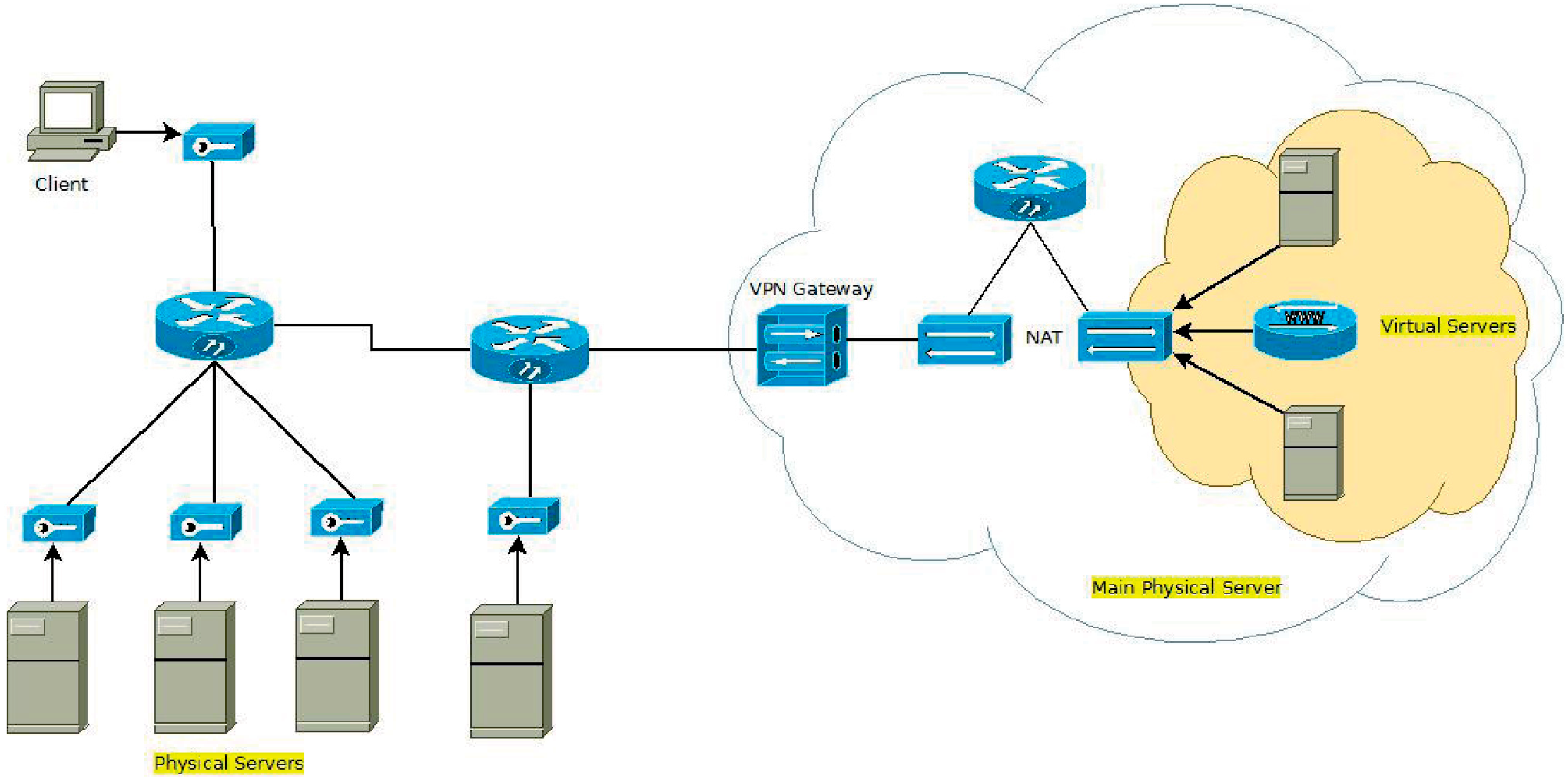
In this Section, we illustrate our experimental assessment and analysis that we devised in order to demonstrate the feasibility of our approach, and the effectiveness and the efficiency of our algorithms. The experimental environment used for our experiments is depicted in
Figure 6. In particular, the target cluster comprises five hosts having the hardware described in
Table 1.
Figure 6.
System environment.
Figure 6.
System environment.
Table 1.
Hardware in the cluster of the experimental environment.
Table 1.
Hardware in the cluster of the experimental environment.
| Core Num. | Core Speed (GHz) | HDD | RAM (GB) |
|---|
| 6 | 2.4 | 1 | 6 |
| 8 | 2.4 | 1 | 2 |
| 4 | 2.7 | 1 | 4 |
| 4 | 2.7 | 1 | 4 |
| 4 | 2.7 | 1 | 4 |
In our experimental campaign, we ran tests on top of our cluster in order to verify its functionality and throughput first. These tests give us a baseline that was helpful to tune the cluster through the various configuration options and the schema of tables themselves.
The Yahoo! Cloud Serving Benchmark (YCSB) [
77] was used to run comparable workloads against different storage systems. While primarily built to compare various systems, YCSB is also a reasonable tool for performing an HBase cluster burn-in or performance-oriented tests (e.g., [
78]). To this end, it is necessary to create some tables and load a bunch of test data (selected by the user or randomly generated) into these tables (generally, at least 10
8 rows of data should be loaded). In order to load data, we used the YCSB client tool [
77] by generating a synthetic dataset that comprises 10
12 rows. After loading the data, YCSB permits to run tests with the usage of the CRUD operations in a set of “workloads”. In the YCSB’s semantics, workloads are configuration files containing the percentage of operations to do, how many operations, how many threads should be used, and other useful experimental parameters.
We ran tests on both the default configuration and other tentative configurations by reaching a throughput of 1300 Op/s for reading-like operations and 3500 Op/s for writing-like operations, thus increasing by 50% the performance obtained with the default configurations. It is worth mentioning that, using both the Snappy compression scheme for reducing the size of data tables and Bloom filters for implementing the membership test in the adjacent lists (which may become very large in real-life RDF graphs) contributed in the performance gain heavily.
Table 2 reports the experimental results provided by this experiment, which comprises the impact of communication costs.
Table 2.
Throughput performance.
Table 2.
Throughput performance.
| | Reading-Like Operations | Writing-Like Operations |
|---|
| Throughput (Op/s) | 1300 | 3500 |
After the first series of experiments devoted to assess the throughput of the framework, we focused our attention on the data management capabilities of the framework by introducing an efficient schema and an efficient client capable of uploading and retrieving data efficiently, i.e., based on the effective schema designed. The first solution contemplated an RDBMS(Relational DataBase Management System)-like approach to the schema design while the second one was more akin to NoSQL paradigms. As it will be mentioned later, the second approach is the one that exposes the best during the retrieval phase, lagging behind the first approach for data uploading. Due to the fact that the performance difference, however, was negligible, the second approach was the one to be implemented. To both solutions, all the optimizations about performance increasing discovered during the “load test” phase were applied (i.e., table data Snappy-based compression and Bloom filters).
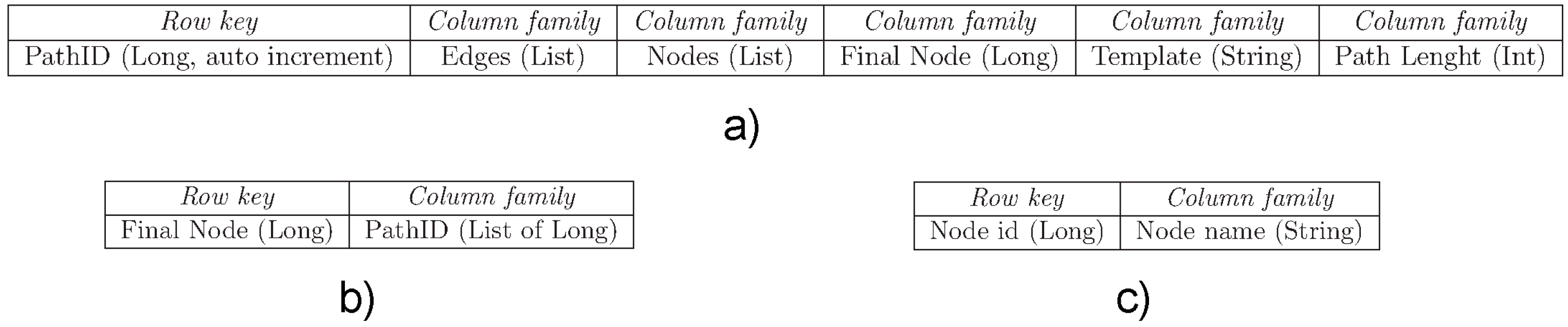
Therefore, we finally implemented three tables for HBase data storage (see
Figure 7). As shown in
Figure 7, the following tables have been devised: (i) table Path, shown in
Figure 7a, is a repository of paths containing all the data modeling a path (
i.e.,
Row key,
Column family,
etc.); (
ii) for each sink, table Sink-Path, shown in
Figure 7b, contains the list of the path IDs (related to the first table) that ends with that node; (
iii) for each node, table Node-Label, shown in
Figure 7c, contains the labels of each node.
Figure 7.
HBase configuration for the running experiment: (a) table Path; (b) table Sink-PathID; (c) table Node-Label.
Figure 7.
HBase configuration for the running experiment: (a) table Path; (b) table Sink-PathID; (c) table Node-Label.
On top of this HBase data storage, we ran simple operations like Get, Batch and Scan, of course being the framework running our proposed algorithm. This allowed us to retrieve one million (1M) of rows within 5.5 ms through
cold-cache experiments and within 1.3 ms through
warm-cache experiments.
Table 3 reports these results.
Table 3.
Data management performance.
Table 3.
Data management performance.
| | Cold-Cache Mode | Warm-Cache Mode |
|---|
| Retrieval Time for 1 M Rows (ms) | 5.5 | 1.3 |
Finally, by analyzing our experimental results, we conclude that our framework for computing BSF-based traversals of RDF graphs clearly exposes both effectiveness and efficiency. As future extension, in order to further improve performance, the proposed framework could be implemented on top of the well-known
Apache Spark analytical engine [
79], as Spark exposes an optimized in-memory computation scheme for large-scale data processing. This would allow us to improve response times.


