3.1. Motivation
Simulation results on several symmetric TSP benchmarks in [
28] illustrate that OBBO seems to be relatively good at optimal solutions when compared with BBO. However, these experiments expose two serious problems, which may indicate that the initial conclusion is questionable.
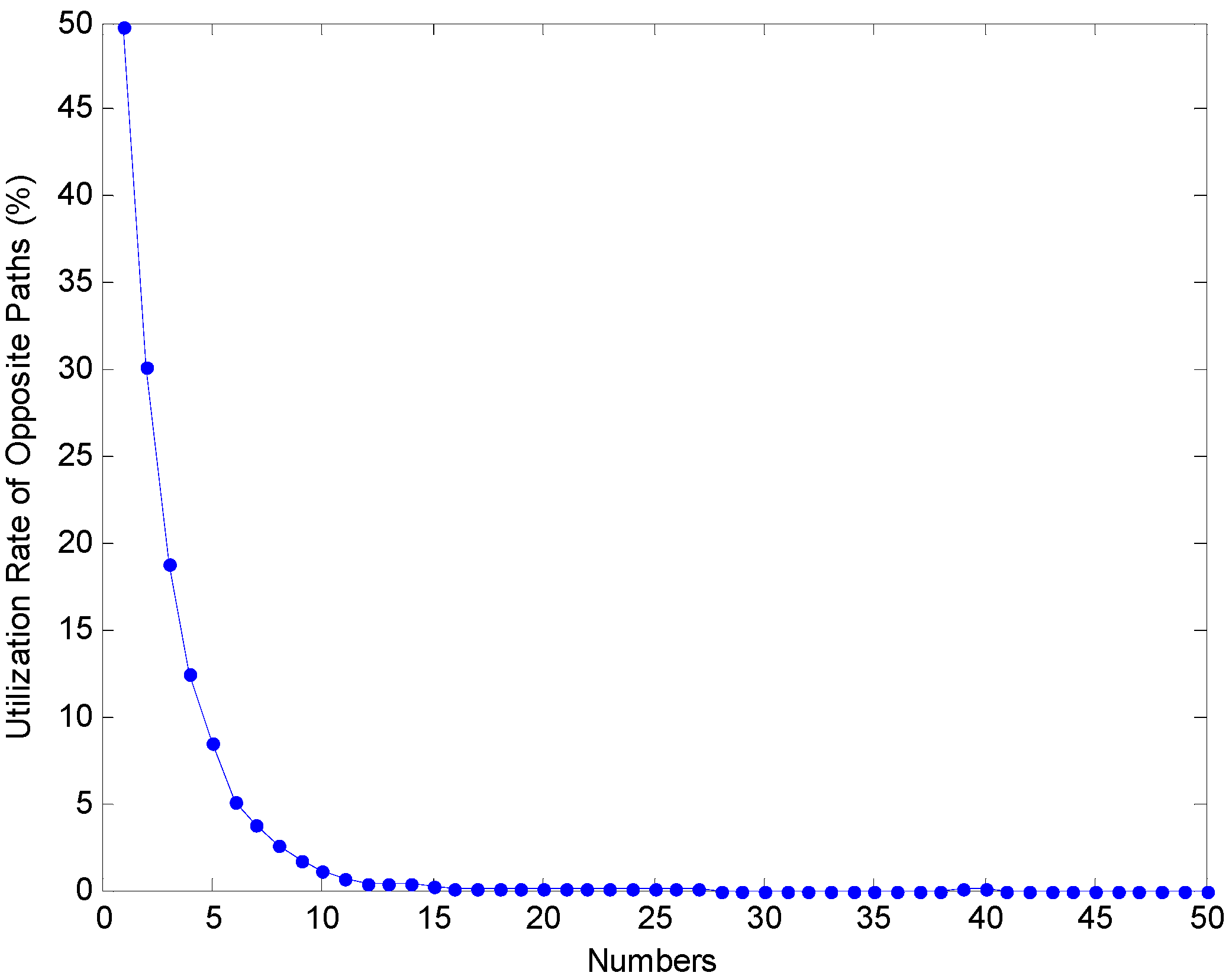
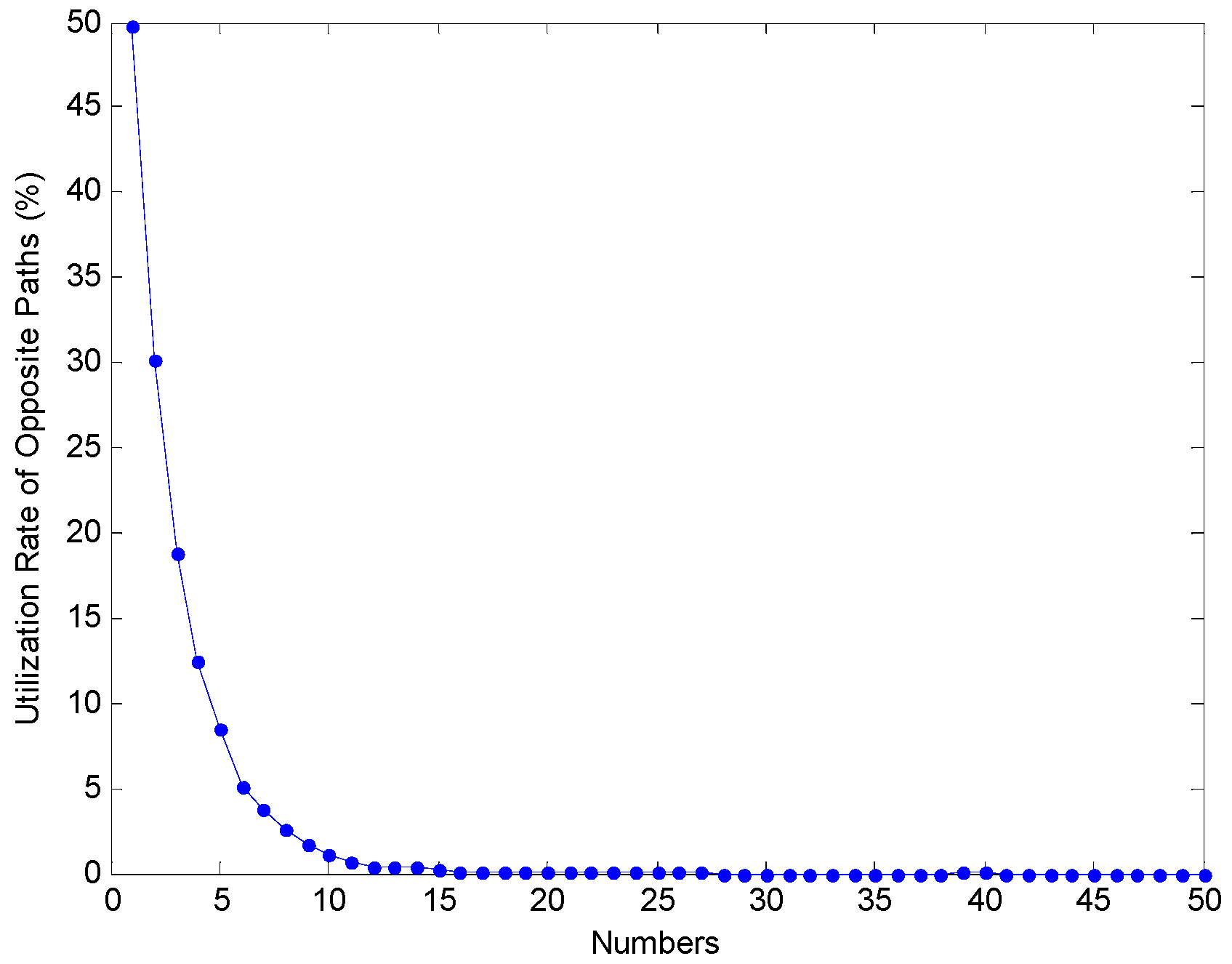
Although the terminal condition is set as a constant generation maximum for different comparison algorithms, such as 500 in that paper, the number of candidate solutions explored in a search space by different algorithms may be well-distinguished between each other. It is intuitively obvious that some opposite paths are explored and then considered in each generation for OBBO algorithm, but not for BBO algorithm. Obviously, to compare the performance of BBO and OBBO algorithm, it is unfair and inadvisable scheme, which instead by our termination criterion in
Section 4.1.
The other problem, hidden behind OBBO for TSP problems, is that the definition of opposite path is too simple to embody some important characteristics of the candidate path. According to our observations and understanding, the city sequences and the distances between adjacent cities are both the two most core features of a TSP path. It is to be noted clearly that the city sequences here means the relative order in TSP path alone. For example, we only concerned that city 25 is former than city 49, and latter than city 12 in a given TSP path (…, 12, 25, 49, …). However, we do not care about the coordinate of the cities 25, 49 and 12, not to mention the Euclidean distances between them. Furthermore, the Euclidean distance is directly computed based on the geometric coordinates of the nodes of the graph, and yet these TSP paths are differentiated by the sequences when only a graph is given. However, the authors used the former feature (city sequences) and ignored the latter one (distances between adjacent cities) unconsciously or consciously, when they defined the opposite path in [
28]. Usually, using the original definition of opposite path presented in [
28] will lead inevitably to the low utilization rate of opposite paths as shown in
Section 4.2.
It is obvious that the definition of opposite path can be considered as a key to promote the opposition-based soft computing for solving TSP problem. Therefore, an initial motivation of this paper is to further amend the definition of opposite path with the help of the Euclidean distances and city sequences in the graph.
Therefore, the next question is that how to use together with Euclidean distances and city sequences of a candidate path. We think Opposition-Based Learning using the Current Optimum, a significant important variation of OBL in continuous domain, might be a good choice by careful observation of these definitions. As mentioned previously, it was first proposed for function optimization as follows [
7].
Definition 3. Let
P = (
x1,
x2, …,
xD) be a point in
D-dimensional space, where
x1,
x2, …,
xD R and
xi [
ai,
bi],
i {1, 2, …,
D}. The opposite point using the current optimum
= (
,
, …,
) is completely defined by its coordinates
where
xco is the optimum solution in the current population.
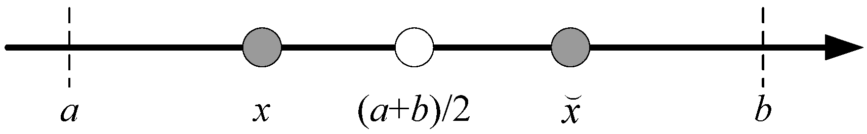
This definition has similarity, in style, with definition 1 proposed by Tizhoosh, but you will find that the opposite point using the current optimum may be outside the range of valid numbers defined by [ai, bi] if you analyze it carefully. Therefore, the possible solutions include recomputing based on Equation (3) until the new one falls in the range of valid numbers, reproducing a random point, and even using the left or right boundary of valid numbers as an alternative.
Figure 2 illustrates the opposite point using the current optimum
in one dimensional case.
Figure 2.
Opposite point using the current optimum defined in domain [a, b]. x is a candidate solution, is the opposite of x and is its opposite using the current optimum.
Figure 2.
Opposite point using the current optimum defined in domain [a, b]. x is a candidate solution, is the opposite of x and is its opposite using the current optimum.
The core idea of COOBL may be summarized as that the optimum solution in the current population, replacing the midpoint in a range of variables’ current interval, is used as symmetry point of the points and their opposite points. As a result, the opposite points using the current optimum will be in the neighborhood of the global optimum during the process of evolution, especially in the later stage.
In this paper, to redefine the opposite path in discrete domain, the candidate solution and the optimum solution in the current population will be also taken into consideration simultaneity in the similar way.
3.2. Definition of Opposite Path using the Current Optimum
In order to achieve a better solution of TSP efficiently, we modify the definition of opposite path as follows.
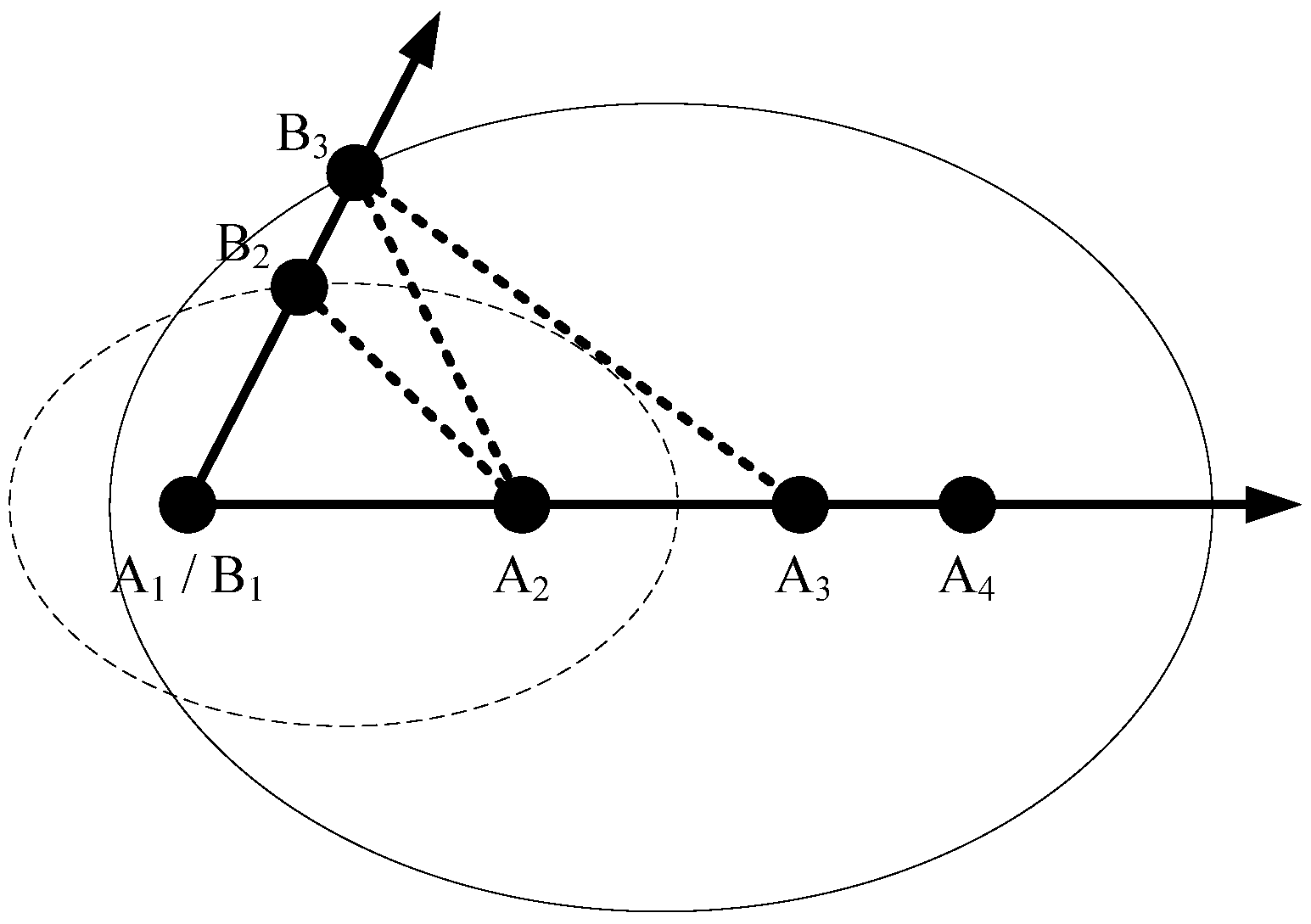
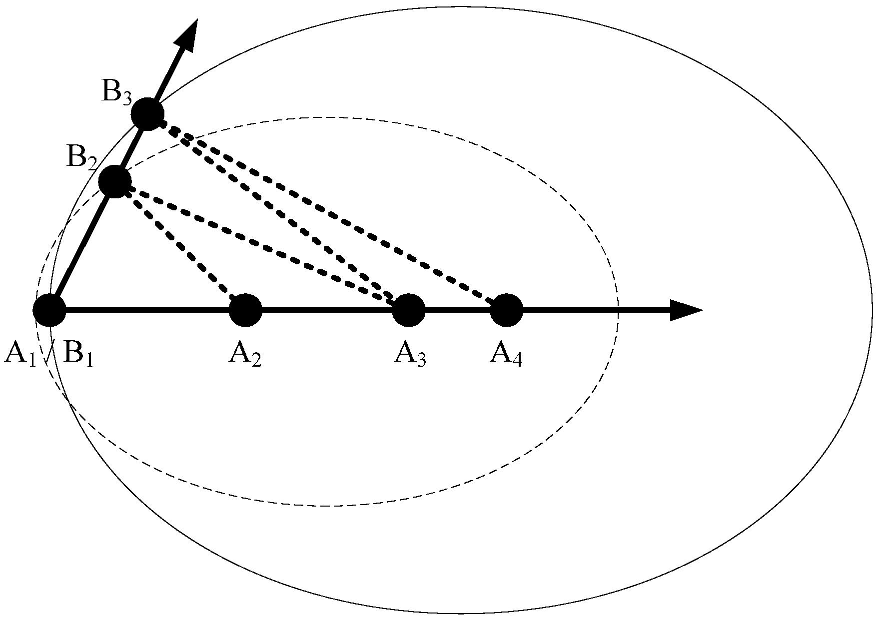
As in
Figure 3, it is supposed that,
n is the number of nodes in a graph and
m is the population size. In fact, this figure can decomposed into three parts to comprehend the novel definition of opposite path clearly, which are shown in
Figure 4. The first part, the optimal path in the current population
Pco = [A
1, A
2, …, A
1], as seen in
Figure 4a is translated into line A
1A
4 in
Figure 3. In addition, similarly, the candidate path
Pi = [B
1, B
2, …, B
1] as the second part of
Figure 3 is also translated into line B
1B
3. The clearly common ground between two important parts of
Figure 3 is that, they are curves in
Figure 4, instead, they are lines in
Figure 3. The only reason for the different expression of the same TSP paths is to simplify the most critical figure in this paper. Based on the similar reason, the third part of
Figure 3, all cities in the graph as seen in
Figure 4c, is ignored in
Figure 3. Of cause, you can image it is ubiquity for all cities in this graph in order to understand the following procedure easily.
Figure 3.
Novel definition of opposite path (Backward Ellipse).
Figure 3.
Novel definition of opposite path (Backward Ellipse).
Figure 4.
Component elements of opposite path (Backward Ellipse). (a) Optimal path in the current population. (b) Candidate path. (c) Cities in the graph.
Figure 4.
Component elements of opposite path (Backward Ellipse). (a) Optimal path in the current population. (b) Candidate path. (c) Cities in the graph.
Based on the preliminary and explanation above, the opposite path (Backward Ellipse), Pio = [O1, O2, …, O1], of any path Pi = [B1, B2, …, B1] can be defined according to the following procedure.
(1) A set of remaining nodes include all nodes in the graph, and a set of visited nodes is empty in initialization stage.
(2) Let k = 1. The start city, A1(B1) of optimal path Pco is also determined as the first node of path Pi and its opposite path Pio. Then A1(B1) is labeled as a visited node and deleted from the set of remaining nodes.
(3) Let k = k + 1. An ellipse is determined and denoted by Ek, in which the (k − 1)th node and kth node of the optimal path Pco are the left focus and the right focus of the ellipse, respectively, and the kth node of Pi is on the boundary of the ellipse Ek.
(4) The kth node Ok of opposite path Pio is the nearest node from the set of remaining nodes to the boundary of the ellipse Ek. Then the kth node is labeled as a visited node and deleted from the set of remaining nodes.
(5) Steps 3 and 4 above are iterated until all nodes are included in the set of visited nodes. Then the opposite path, Pio, of any path Pi is defined well.
As stated above, the ellipse Ek is determined by means of the (k − 1)th node, the kth node of the optimal path Pco and the kth node of Pi. The kth node of opposite path Pio is close to the boundary of the ellipse Ek. In other words, the kth node of Pi and the kth node of opposite path Pio have the same (or similar at least) distance from the (k − 1)th node and the kth node of the optimal path Pco. Further, the (k − 1)th node and the kth node of the optimal path Pco can take the place of the whole optimal path Pco. Then the path Pi and its corresponding opposite path Pio have the same (or similar at least) distance to the whole optimal path Pco in the current population in a sense.
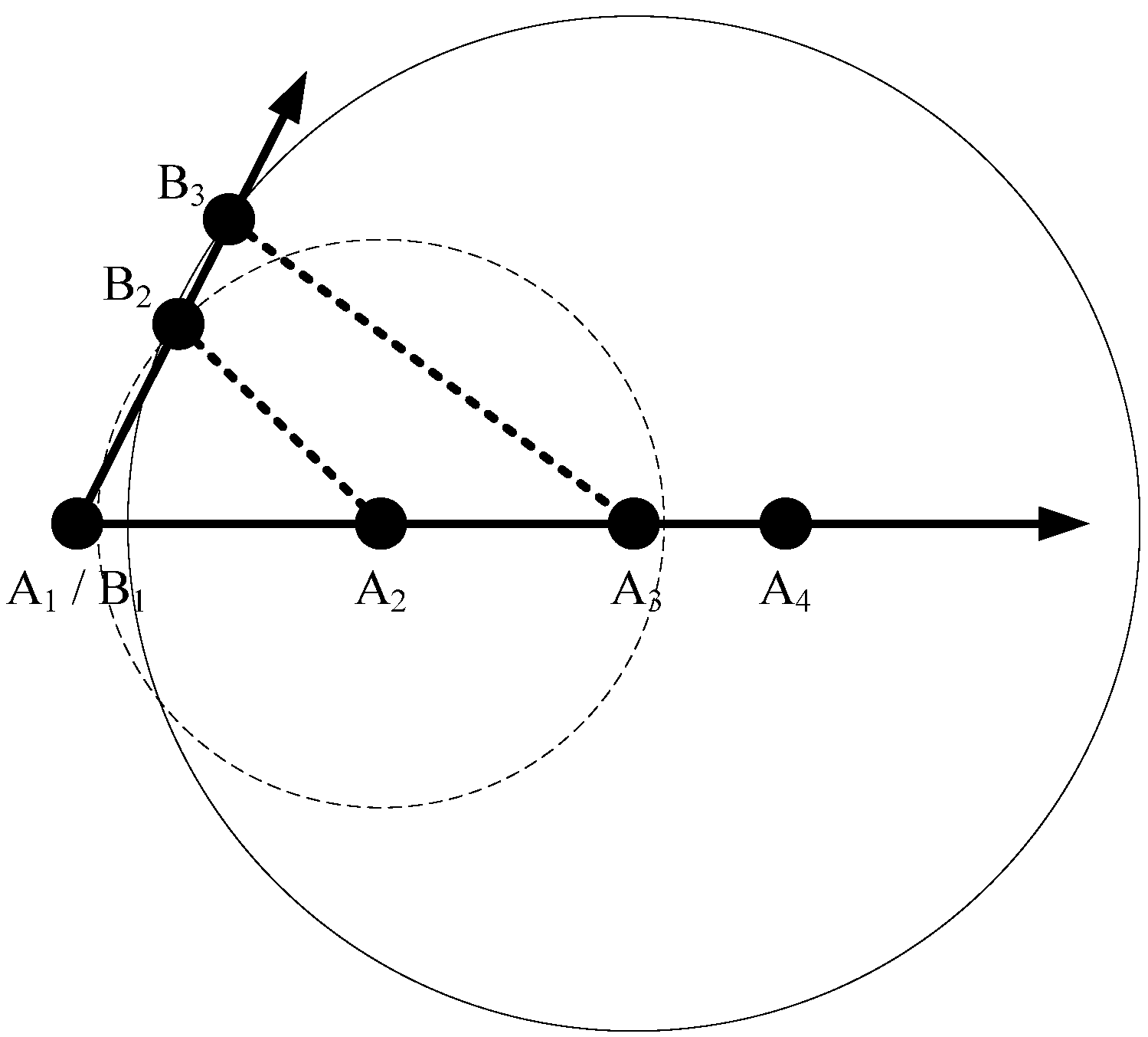
Quite similarly, we can define the other two methods, opposite path (Forward Ellipse) and opposite path (Circle), as shown in
Figure 5 and
Figure 6, respectively. For opposite path (Forward Ellipse), the ellipse
Ek is determined by means of the
kth node, the (
k + 1)th node of the optimal path
Pco and the
kth node of
Pi. For instance, the second node O
2 of opposite path
Pio and node B
2 of
Pi have the same/similar distance from nodes A
2 and A
3 of the optimal path
Pco. The third node O
3 of opposite path
Pio and node B
3 of
Pi have the same/similar distance from nodes A
3 and A
4 of the optimal path
Pco, and so on. For opposite path (Circle), the ellipse
Ek is degenerated into a circle
Ck, in which the center is the
kth node of the optimal path
Pco and the radius is the distance between the center and the
kth node of
Pi. For instance, the node B
2 of
Pi is located at the boundary of the circle
C2 and the second node O
2 of opposite path
Pio is selected around the boundary. The node B
3 is located at the boundary and the node O
3 is selected around the boundary of the circle
C3, and so on.
Figure 5.
Novel definition of opposite path (Forward Ellipse).
Figure 5.
Novel definition of opposite path (Forward Ellipse).
Figure 6.
Novel definition of opposite path (Circle).
Figure 6.
Novel definition of opposite path (Circle).
Without a doubt we introduce the information of the optimum solution in the current population, including the Euclidean distances and the node sequences, into all definitions of opposite path in this paper. The path and its corresponding opposite path have the similar distance to the current optimum in a sense. In addition, the node sequences of opposite path are nearly kept with the original path and optimal path in order, although the direction of opposite path may be slightly different with the original path. In a word, our definition method of opposite path, which is significantly different from [
28], considers both the node sequences of candidate paths and the distances between adjacent nodes at the same time. In my opinion, it may be a novel and promising attempt to applying the opposition-based soft computing in discrete domain.


