Improving Man-Optimal Stable Matchings by Minimum Change of Preference Lists ^†

Abstract

In the stable marriage problem, any instance admits the so-called man-optimal stable matching, in which every man is assigned the best possible partner. However, there are instances for which all men receive low-ranked partners even in the man-optimal stable matching. In this paper we consider the problem of improving the man-optimal stable matching by changing only one man’s preference list. We show that the optimization variant and the decision variant of this problem can be solved in time $O\left(n^3\right)$ and $O\left(n^2\right)$, respectively, where n is the number of men (women) in an input. We further extend the problem so that we are allowed to change k men’s preference lists. We show that the problem is W[1]-hard with respect to the parameter k and give $O\left(n^{2k+1}\right)$-time and $O\left(n^{k+1}\right)$-time exact algorithms for the optimization and decision variants, respectively. Finally, we show that the problems become easy when $k=n$; we give $O(n^{2.5}logn)$-time and $O\left(n^2\right)$-time algorithms for the optimization and decision variants, respectively.

1. Introduction

An instance of the stable marriage problem [1] consists of the same number n of men and women, and each person’s preference list. In a preference list, each person ranks all the members of the opposite sex in a strict order. A matching is a set of n disjoint man–woman pairs in which each person appears exactly once. A blocking pair for a matching M is a man–woman pair each of whom prefers the other to his/her partner in M. A matching is stable if it contains no blocking pair.

It is known that there exists at least one stable matching in any instance, and one can be found by the Gale–Shapley algorithm (GS) in $O\left(n^2\right)$ time [1,2]. The stable matching found by GS is called the man-optimal stable matching that has an extreme property that every man is assigned the best possible partner among all the stable matchings. In applications for asymmetric settings, such as assigning residents to hospitals or students to schools, it is common to formulate the problem by setting residents or students to the men’s side, so that those people can receive benefit. Nevertheless, there are instances for which all (or almost all) men are assigned low-ranked partners even in the man-optimal stable matching, (e.g., a worst case instance for GS given in Figure 1, which originates from [2]). For such instances, the merit of using the man-optimal mechanism cannot be sufficiently exploited.

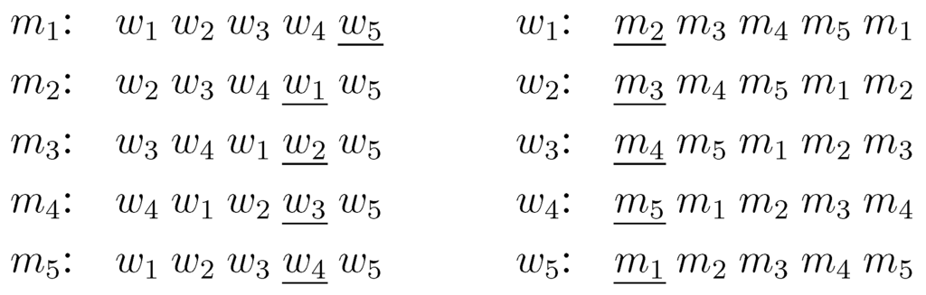
Figure 1. Worst case example for the Gale–Shapley algorithm for $n=5$. Partners in the man-optimal stable matching are underlined. Each preference list is ordered from left to right in increasing order of the rank, i.e., the leftmost person is the most preferable and the rightmost person is the least preferable.

To overcome this drawback, we consider the problem of improving the man-optimal stable matching by allowing small changes in preference lists. In this paper we first allow only one man’s preference list to be changed, and consider optimization and decision variants. In the optimization variant, we are asked to find a man and a way of changing his list that cause the maximum improvement. In the decision variant, we ask if we can obtain a positive improvement. For both problems, we impose a restriction that no man should be assigned a worse partner than the man-optimal partner in the original instance. We show that these problems can be solved in time $O\left(n^3\right)$ and $O\left(n^2\right)$, respectively. We then extend the problem so that we are allowed to change k men’s preference lists. We show that the optimization variant is W[1]-hard with respect to the parameter k. We also give $O\left(n^{2k+1}\right)$-time and $O\left(n^{k+1}\right)$-time exact algorithms for the optimization and decision variants, respectively. Finally, we show that the problems become easy when $k=n$, i.e., we are allowed to change the preference lists of any number of men. We give $O(n^{2.5}logn)$-time and $O\left(n^2\right)$-time algorithms for the optimization and decision variants, respectively.

Our problem can also be viewed as an issue of coalition strategy by men. Knowing all the preference lists, men are trying to maximize their total profit by submitting falsified preference lists, while bounding the number of such liars and guaranteeing that no one becomes worse off. Results of this paper show the computational complexities of obtaining an optimal strategy depending on the number k of liars. Strategic issue in the stable marriage problem is an extensively studied topic (see [3] for example).

2. Preliminaries

2.1. Problem Definitions

Let I be an instance of the stable marriage problem. In this paper, we consider only complete preference lists with no ties. The rank of a woman w in man m’s preference list, denoted $r_m\left(w\right)$, is one plus the number of women that precede w in m’s list. For a matching M and a person p, let $M\left(p\right)$ be p’s partner in M. The score of m in M is the rank of his partner in M, i.e., $r_m\left(M\left(m\right)\right)$. The score of M is the sum of the scores of all men, i.e., ${\sum }_m{r}_m\left(M\left(m\right)\right)$. The man-optimal score of I, denoted $MO\left(I\right)$, is the score of the man-optimal stable matching $M_0$ of I.

Let k be a positive integer. If $\tilde{I}$ is an instance obtained by changing the preference lists of at most k men in I in some way, then we say that $\tilde{I}$ is a k-neighbor of I. Suppose that $\tilde{I}$ is a k-neighbor obtained by changing the preference lists of $\widetilde{m_1},\widetilde{m_2},\dots ,\widetilde{m_{\ell }}$ ($\ell \le k$) and let $\widetilde{M_0}$ be the man-optimal stable matching for $\tilde{I}$. The man-optimal score of $\tilde{I}$ with respect to I, denoted $M{O}_I\left(\tilde{I}\right)$, is the score of $\widetilde{M_0}$ where $\widetilde{m_1},\widetilde{m_2},\dots ,\widetilde{m_{\ell }}$’s scores are measured in terms of their preference lists in I. (Intuitively, their scores are measured in their true preference lists.) We say that $\tilde{I}$ is proper if each man receives at least as good a partner in $\widetilde{M_0}$ as in $M_0$, i.e., $r_m(\widetilde{M_0}(m))\le r_m\left(M_0\left(m\right)\right)$ for each m, where $\widetilde{m_1},\widetilde{m_2},\dots ,\widetilde{m_{\ell }}$’s scores are measured in their preference lists in I.

The problem MAX MAN-OPT IMPROVE(k) (MMI(k) for short) is, given a stable marriage instance I, to find a proper k-neighbor $\tilde{I}$ of I such that $MO\left(I\right)-M{O}_I\left(\tilde{I}\right)$ is maximized. The problem POSITIVE MAN-OPT IMPROVE(k) (PMI(k) for short) is to determine if there is a proper k-neighbor $\tilde{I}$ of I such that $MO\left(I\right)-M{O}_I\left(\tilde{I}\right)>0$.

2.2. Reduced Lists and Rotation Digraphs

In constructing algorithms and proving W[1]-hardness, we use reduced lists and rotation digraphs. These are defined on an instance I and its stable matching M, and are constructed in the following way: For each man m and each woman w below $M\left(m\right)$ in m’s preference list, delete w from m’s list and m from w’s list. The resulting preference lists are called the woman-oriented reduced lists with respect to I and M, denoted $R{L}_{I,M}$. (We may simply call them the reduced lists if there is no ambiguity). Note that for each woman w, $M\left(w\right)$ lies at the top of w’s reduced list since M is stable. For each woman w, let $nex{t}_{I,M}\left(w\right)$ be the man at the second position of w’s reduced list (if any). The woman-oriented rotation digraph with respect to I and M (or simply the rotation digraph) is a digraph $D_{I,M}=(V,A)$ where V is the set of men and A includes an arc $(M\left(w\right),nex{t}_{I,M}\left(w\right))$ (i.e., a directed edge from $M\left(w\right)$ to $nex{t}_{I,M}\left(w\right)$) for each woman w such that $nex{t}_{I,M}\left(w\right)$ exists. Suppose that there is a directed cycle $m_0,m_1,\dots ,m_{r-1}$ ($r\ge 2$) in $D_{I,M}$, and let $w_i=M\left(m_i\right)$ for all i ($0\le i\le r-1$). Then we call an ordered list of pairs $\rho =(m_0,w_0),(m_1,w_1),\dots ,(m_{r-1},w_{r-1})$ a rotation exposed in M. If we modify M by removing the pairs of rotation ρ and adding $(m_i,w_{i-1\text{mod}r})$ for each i, then the resulting matching is also stable [2]. In this case we say that the new matching is obtained by eliminating the rotation ρ from M. Note that by eliminating a rotation, every man in the rotation obtains a better partner, while every woman in the rotation obtains a worse partner. It is also known that M is the man-optimal stable matching of I if and only if there is no rotation exposed in M (or equivalently, $D_{I,M}$ has no directed cycle) [2].

3. Changing One Man’s Preference List

3.1. Optimization Variant

Let I be a given instance and $M_0$ be its man-optimal stable matching. Let us fix a man m whose preference list is to be changed. The following proposition, due to Huang [3], is useful for our purpose. Recall that a preference list is ordered from left to right in increasing order of the rank.

Proposition 3.1 

[3] Let $P_L\left(m\right)M_0\left(m\right)P_R\left(m\right)$ be m’s preference list in I, where $P_L\left(m\right)$ ($P_R\left(m\right)$) denotes the left (right) part of $M_0\left(m\right)$ in m’s list. Let $I^{\prime }$ be an instance constructed in the following way: Take any number of women from $P_L\left(m\right)$, move them to the right of $M_0\left(m\right)$, and arbitrarily permute each of the (new) left and right parts of $M_0\left(m\right)$. Let $M_0^{\prime }$ be the man-optimal stable matching for $I^{\prime }$. Then in $M_0^{\prime }$ no man is worse off than in $M_0$ (with respect to preference order of I).

Then we can claim that there is an optimal solution in which $M_0\left(m\right)$ lies at the top of m’s list for the following reason: Note that m cannot be matched with a woman worse than $M_0\left(m\right)$ by the requirement of the problem. On the other hand, it is shown in [2] (page 56, Theorem 1.7.1) that m cannot get a better man-optimal partner by falsifying his preference list. Hence, in any feasible solution, m must be matched with $M_0\left(m\right)$. If $M_0\left(m\right)$ is not at the top of m’s list in some feasible solution, we can move women on the left of $M_0\left(m\right)$ to the right of $M_0\left(m\right)$ without increasing the man-optimal score, by Proposition 3.1. Hence our claim holds. Since m is matched with $M_0\left(m\right)$ in a feasible solution, the order of women other than $M_0\left(m\right)$ in m’s list is not important. Hence all we need to do is to move $M_0\left(m\right)$ to the top of m’s list, which implies the following simple Algorithm 1.

Example. 

We give an example of the execution of Algorithm 1 for instance I given in Figure 1. The man-optimal stable matching $M_0$ is given in Figure 1 and $MO\left(I\right)=21$. At line 2, we first consider $m_1$. At line 3, we construct an instance $I_{m_1}$ by moving $w_5$ to the top of $m_1$’s list. By applying GS, we find that the man-optimal stable matching of $I_{m_1}$ is $M_{m_1}=\{(m_1,w_5),(m_2,w_2),(m_3,w_3),(m_4,w_4),(m_5,w_1)\}$ and $M{O}_I\left(I_{m_1}\right)=9$. Next, we consider $m_2$. The instance $I_{m_2}$ is constructed by moving $w_1$ to the top of $m_2$’s list. The man-optimal stable matching of $I_{m_2}$ is also $M_0$ and $M{O}_I\left(I_{m_2}\right)=21$. By continuing this, we can find that $M{O}_I\left(I_{m_3}\right)=M{O}_I\left(I_{m_4}\right)=M{O}_I\left(I_{m_5}\right)=21$. Hence, Algorithm 1 outputs $I_{m_1}$ since $M{O}_I\left(I_{m_1}\right)$ is the smallest.

   ☐

Algorithm 1:

1: Find the man-optimal stable matching M0 of I.

2: for each man m do

3:  Modify I by moving M0(m) to the top of m’s list. Let Im be the resulting instance.

4:  Apply GS to Im and find its man-optimal stable matching Mm.

5: end for

6: Let m* be a man such that the score of Mm* is minimum.

7: Output Im* .

Since GS runs in time $O\left(n^2\right)$, line 1 and the body of the for loop can be executed in time $O\left(n^2\right)$. Since there are n men, the overall time complexity of Algorithm 1 is $O\left(n^3\right)$.

Theorem 3.2 

MMI(1) can be solved in $O\left(n^3\right)$ time.

3.2. Decision Variant

Note that a direct application of Algorithm 1 solves PMI(1) in $O\left(n^3\right)$ time. We improve this to $O\left(n^2\right)$ using a structural property of stable matchings. Let I be an input. From the discussion in Section 3.1, it suffices to consider the instance $I_m$ for each man m (see the description of Algorithm 1 for the definition of $I_m$.) It is not hard to see that the man-optimal stable matching $M_0$ of I is also stable in $I_m$ for any m. Hence, if $M_0$ is not the man-optimal stable matching of $I_m$ for some m, then the man-optimal stable matching of $I_m$ is better than $M_0$, so the answer is “yes”; otherwise, the answer is “no”. To check whether $M_0$ is the man-optimal stable matching of $I_m$ or not in time $O\left(n\right)$ per man, we use the woman-oriented rotation digraphs defined in Section 2.2.

Given I, we construct the rotation digraph $D_{I,M_0}$ with respect to the man-optimal stable matching $M_0$. Clearly it is acyclic. For a man m, we construct the instance $I_m$ (defined before) and the rotation digraph $D_{I_m,M_0}$ (recall that $M_0$ is stable in $I_m$ and hence $D_{I_m,M_0}$ is defined). From the discussion in Section 2.2, we know that $M_0$ is the man-optimal stable matching of $I_m$ if and only if $D_{I_m,M_0}$ contains no cycle. Hence our task can be reduced to checking if $D_{I_m,M_0}$ contains a cycle. The pseudocode of our algorithm is given as Algorithm 2:

Algorithm 2:

1: Find the man-optimal stable matching M0 of I.

2: Construct DI,M0 .

3: for each man m do

4:  Modify I by moving M0(m) to the top of m’s list. Let Im be the resulting instance.

5:  Construct DIm,M0 .

6:  if DIm,M0 contains a cycle then

7:   Output “yes” and terminate.

8:  end if

9: end for

10: Output “no”.

Example. We give an example of the execution of Algorithm 2 for instance I of Figure 1. The man-optimal stable matching $M_0$ is depicted in Figure 1. In constructing the reduced lists $R{L}_{I,M_0}$, we delete $w_5$ from $m_2,m_3,m_4$, and $m_5$’s lists, and $m_2,m_3,m_4$, and $m_5$ from $w_5$’s list. Hence $R{L}_{I,M_0}$ is as follows:

m1:  w1 w2 w3 w4 w5	w1:  m2 m3 m4 m5 m1
m2:  w2 w3 w4 w1	w2:  m3 m4 m5 m1 m2
m3:  w3 w4 w1 w2	w3:  m4 m5 m1 m2 m3
m4:  w4 w1 w2 w3	w4:  m5 m1 m2 m3 m4
m5:  w1 w2 w3 w4	w5:  m1

The rotation digraph $D_{I,M_0}$ has four arcs $(m_2,m_3)$, $(m_3,m_4)$, $(m_4,m_5)$, and $(m_5,m_1)$, as illustrated in Figure 2(a).

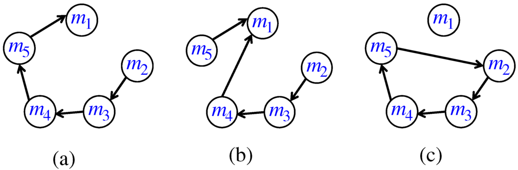
Figure 2. Rotation digraphs.

For a better exposition, let us first choose $m_5$ at line 3. To construct $I_{m_5}$, we move $w_4$ to the top of $m_5$’s list. We then delete $w_1$, $w_2$, and $w_3$ from $m_5$’s list and $m_5$ from $w_1$, $w_2$, and $w_3$’s lists in $R{L}_{I,M_0}$, and we obtain the following $R{L}_{I_{m_5},M_0}$:

m1:  w1 w2 w3 w4 w5	w1:  m2 m3 m4 m1
m2:  w2 w3 w4 w1	w2:  m3 m4 m1 m2
m3:  w3 w4 w1 w2	w3:  m4 m1 m2 m3
m4:  w4 w1 w2 w3	w4:  m5 m1 m2 m3 m4
m5:  w4	w5:  m1

To construct the rotation digraph $D_{I_{m_5},M_0}$, we remove an arc $(m_4,m_5)$ from $D_{I,M_0}$ and add $(m_4,m_1)$ because $nex{t}_{I,M_0}\left(w_3\right)=m_5$ but $nex{t}_{I_{m_5},M_0}\left(w_3\right)=m_1$. The resulting $D_{I_{m_5},M_0}$ is depicted in Figure 2(b). This digraph $D_{I_{m_5},M_0}$ contains no cycle and hence we proceed to the next man.

Next, suppose that we choose $m_1$ at line 3. Then $R{L}_{I_{m_1},M_0}$ is as follows:

m1:  w5	w1:  m2 m3 m4 m5
m2:  w2 w3 w4 w1	w2:  m3 m4 m5 m2
m3:  w3 w4 w1 w2	w3:  m4 m5 m2 m3
m4:  w4 w1 w2 w3	w4:  m5 m2 m3 m4
m5:  w1 w2 w3w4	w5:  m1

To construct the rotation digraph $D_{I_{m_1},M_0}$, we remove an arc $(m_5,m_1)$ from $D_{I,M_0}$ and add $(m_5,m_2)$ and obtain $D_{I_{m_1},M_0}$ in Figure 2(c). Since $D_{I_{m_1},M_0}$ contains a cycle, Algorithm 2 outputs “yes” and terminates.    ☐

Lines 1 and 2 can be performed in time $O\left(n^2\right)$. Checking whether $D_{I_m,M_0}$ contains a directed cycle or not can be done by a standard topological sorting algorithm in time linear in the size of $D_{I_m,M_0}$. Since each vertex of $D_{I_m,M_0}$ has outdegree at most one, the size of $D_{I_m,M_0}$ is $O\left(n\right)$ and line 6 can be done in $O\left(n\right)$ time. Shortly, we show that $D_{I_m,M_0}$ can be constructed from $D_{I,M_0}$ in time $O\left(n\right)$. Then the overall time complexity of Algorithm 2 is $O\left(n^2\right)$.

Note that the reduced lists $R{L}_{I_m,M_0}$ can be constructed from $R{L}_{I,M_0}$ by deleting each woman w who precedes $M_0\left(m\right)$ from m’s preference list, and correspondingly m from w’s list. If m is not $nex{t}_{I,M_0}\left(w\right)$, then $nex{t}_{I_m,M_0}\left(w\right)=nex{t}_{I,M_0}\left(w\right)$. Otherwise, i.e., if $nex{t}_{I,M_0}\left(w\right)=m$, then the man (say, $m^{\prime }$) at the third position of $R{L}_{I,M_0}$ (if any) will be at the second position of $R{L}_{I_m,M_0}$, i.e., $nex{t}_{I_m,M_0}\left(w\right)=m^{\prime }$. Accordingly we must replace the directed edge $(M_0\left(w\right),m)$ by $(M_0\left(w\right),m^{\prime })$. By doing this for every such w, we can obtain $D_{I_m,M_0}$ in time $O\left(n\right)$.

Theorem 3.3 

PMI(1) can be solved in $O\left(n^2\right)$ time.

4. Changing k Men’s Preference Lists

4.1. Hardness Result

In this section, we show W[1]-hardness of MMI(k). This hardness implies that MMI(k) probably does not admit an FPT algorithm with parameter k, i.e., an $O\left(f\right(k)·p(n\left)\right)$-time algorithm where f is any function and p is a polynomial.

Theorem 4.1 

MMI(k) with parameter k is W[1]-hard.

Proof. 

The Densest k Subgraph problem (DkS) [4] is the following problem. We are given a graph G and a positive integer k. The task is to find an induced subgraph of G with k vertices that contains the maximum number of edges. It is known that DkS is W[1]-hard with parameter k [5]. We give an FPT-reduction from DkS to MMI(k).

Given an instance $(G,k_1)$ of DkS, we construct an instance $(I,k_2)$ of MMI(k) as follows. First, we let $k_2=k_1$. Next, we construct I from $G=(V,E)$. For each vertex $v_i\in V$, we construct a man $m_i$ and a woman $w_i$. For each edge $(v_i,v_j)\in E$, we construct two men $m_{i,j}$ and $m_{i,j}^{\prime }$ and two women $w_{i,j}$ and $w_{i,j}^{\prime }$. For a vertex $v_i\in V$, let $E_i\subseteq E$ be the set of edges incident to $v_i$ and $W_i$ be the set of women $w_{i,j}$ corresponding to $E_i$. Each person’s preference list is constructed as follows, where $L\left(W_i\right)$ is an arbitrarily ordered list of women in $W_i$ and “⋯” means an arbitrarily ordered list of those people who do not appear explicitly in the list.

mi:  L(Wi) wi …	(1 ≤ i ≤ |V|)	wi:  mi …	(1 ≤ i ≤ |V|)
mi,j:  $w_{i,j}^{\prime }$ wi,j …	((i, j) ∈ E)	wi,j:  mi,j mi mj $m_{i,j}^{\prime }$ …	((i, j) ∈ E)
$m_{i,j}^{\prime }$:  wi,j $w_{i,j}^{\prime }$ …	((i, j) ∈ E)	$w_{i,j}^{\prime }$:  $m_{i,j}^{\prime }$ mi, j …	((i,j) ∈ E)

It is not hard to see that the man-optimal stable matching $M_0$ of I consists of pairs $(m_i,w_i)$ for $1\le i\le \left|V\right|$ and $(m_{i,j},w_{i,j})$ and $(m_{i,j}^{\prime },w_{i,j}^{\prime })$ for $(i,j)\in E$. Note that if we ignore the “⋯” part in the above preference lists, each man is matched with the last woman and each woman is matched with the first man in $M_0$. Hence these are the woman-oriented reduced lists with respect to I and $M_0$, i.e., $R{L}_{I,M_0}$.

Clearly, the reduction can be performed in time polynomial in $\left|G\right|$. To complete the proof, we show that G has an induced subgraph with $k_1$ vertices and at least s edges if and only if there is a proper $k_2$-neighbor $\tilde{I}$ of I such that $MO\left(I\right)-M{O}_I\left(\tilde{I}\right)\ge 2s$. Since $k_1=k_2$, in the following we use k to denote $k_1$ and $k_2$ just for simplicity. First, suppose that G has an induced subgraph with k vertices and at least s edges, and let $S(\subseteq V)$ be the set of those k vertices. Then, for each $v_i\in S$, we modify $m_i$’s preference list by moving his man-optimal partner $w_i$ to the top of the list, and let $\tilde{I}$ be the resulting instance. We will show that, by doing this, $m_{i,j}$ and $m_{i,j}^{\prime }$’s scores in the man-optimal stable matching of $\tilde{I}$ are decreased by one respectively, if $v_i,v_j\in S$ and $(v_i,v_j)\in E$. Since there are at least s such edges, the score is decreased by at least $2s$ in total.

Recall that $w_{i,j}$’s reduced list in $R{L}_{I,M_0}$ is “$m_{i,j}$ $m_i$ $m_j$ $m_{i,j}^{\prime }$”. Since $v_i,v_j\in S$ and $m_i$ and $m_j$’s preference lists are modified as mentioned above, $w_{i,j}$’s reduced list in $R{L}_{\tilde{I},M_0}$ becomes “$m_{i,j}$ $m_{i,j}^{\prime }$”, i.e., $nex{t}_{\tilde{I},M_0}\left(w_{i,j}\right)=m_{i,j}^{\prime }$. Note that $w_{i,j}^{\prime }$’s reduced list “$m_{i,j}^{\prime }$ $m_{i,j}$” is unchanged. Then we have a directed cycle $m_{i,j}{m}_{i,j}^{\prime }$ of length two in $D_{\tilde{I},M_0}$ and if we eliminate this rotation, the scores of $m_{i,j}$ and $m_{i,j}^{\prime }$ will each be decreased by one. Note that we can repeat this argument independently for each edge.

Next, suppose that there is a proper k-neighbor $\tilde{I}$ of I such that $MO\left(I\right)-M{O}_I\left(\tilde{I}\right)\ge 2s$ and let $\widetilde{M_0}$ be the man-optimal stable matching of $\tilde{I}$. First, note that in $\widetilde{M_0}$, each man is matched with a woman on the reduced lists $R{L}_{I,M_0}$ because by the condition of the problem, no man can be worse off in $\widetilde{M_0}$ than in $M_0$. Since $\widetilde{M_0}$ is a perfect matching, we know that $\widetilde{M_0}\left(m_i\right)=w_i$ for each i ($1\le i\le \left|V\right|$) and either “$\widetilde{M_0}\left(m_{i,j}\right)=w_{i,j}$ and $\widetilde{M_0}\left(m_{i,j}^{\prime }\right)=w_{i,j}^{\prime }$” or “$\widetilde{M_0}\left(m_{i,j}\right)=w_{i,j}^{\prime }$ and $\widetilde{M_0}\left(m_{i,j}^{\prime }\right)=w_{i,j}$” for each $(v_i,v_j)\in E$. Therefore, only the case of “$\widetilde{M_0}\left(m_{i,j}\right)=w_{i,j}^{\prime }$ and $\widetilde{M_0}\left(m_{i,j}^{\prime }\right)=w_{i,j}$”, the scores of $m_{i,j}$ and $m_{i,j}^{\prime }$ will each be decreased by one. This can happen only when $m_{i,j}^{\prime }$ becomes $nex{t}_{\tilde{I},M_0}\left(w_{i,j}\right)$, that is, $m_i$ and $m_j$ are removed from $w_{i,j}$’s reduced list. This implies that $w_i$ precedes $w_{i,j}$ in $m_i$’s reduced list and $w_j$ precedes $w_{i,j}$ in $m_j$’s reduced list. Therefore, both $m_i$ and $m_j$’s lists are modified in $\tilde{I}$. Since $MO\left(I\right)-M{O}_I\left(\tilde{I}\right)\ge 2s$, there are at least s such pairs $(i,j)$. Let S be the set of vertices $v_i$ such that $m_i$’s preference list is modified in constructing $\tilde{I}$. Then $\left|S\right|\le k$ and by the above discussion, S induces at least s edges, which completes the proof.    ☐

4.2. Optimization Variant

From the discussion in Section 3.1, it seems that it would suffice to choose k men whose preference lists are to be modified, and move their man-optimal partners to the top of their respective preference lists. If this is true, we obtain an $O\left(n^{k+2}\right)$-time algorithm since there are $O\left(n^k\right)$ combinations of selecting k men and for each of them, we run GS whose time complexity is $O\left(n^2\right)$. However, the following example (Figure 3) shows that this is not true.

Nevertheless, the following lemma allows the search space to be bounded.

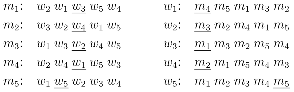
Figure 3. A counter example for the naive algorithm where $k=2$. Man-optimal partners are underlined. An optimal solution is obtained by moving $w_4$ and $w_5$ to the top in $m_4$’s and $m_5$’s preference lists respectively, as a result of which the score decreases by seven. Any choice of two men and moving their man-optimal partners to the top decreases the score by at most five.

Lemma 4.2 

For an instance I, let $I_{opt}$ be an optimal solution and $M_{opt}$ be the man-optimal stable matching of $I_{opt}$. Let S ($\left|S\right|\le k$) be the set of men whose preference lists are modified in $I_{opt}$. Let $\tilde{I}$ be the instance obtained from I by moving $M_{opt}\left(m\right)$ to the top of m’s list for each $m\in S$. Then $M_{opt}$ is stable, and in fact man-optimal stable, for $\tilde{I}$.

Proof. 

Suppose that $M_{opt}$ has a blocking pair in $\tilde{I}$. Each $m\in S$ cannot be a part of a blocking pair because $M_{opt}\left(m\right)$ lies at the top of m’s list. But men not in S and all the women have the same preference list in $I_{opt}$ and $\tilde{I}$, so if $(m^{\prime },w^{\prime })$ is a blocking pair for $M_{opt}$ in $\tilde{I}$, then $(m^{\prime },w^{\prime })$ is also a blocking pair for $M_{opt}$ in $I_{opt}$, a contradiction. Hence $M_{opt}$ is stable for $\tilde{I}$.   ☐

Now suppose that $M_{opt}$ is not man-optimal for $\tilde{I}$ and let $M^{\prime }(\ne M_{opt})$ be the man-optimal stable matching for $\tilde{I}$. Since $M_{opt}$ matches every man in S to his top choice in $\tilde{I}$, so does $M^{\prime }$. Thus some of the men not in S (whose preference lists are the same in I and $\tilde{I}$) obtain better partners in $M^{\prime }$ than in $M_{opt}$. This means that $M{O}_I\left(\tilde{I}\right)<M{O}_I\left(I_{opt}\right)$, which contradicts the optimality of $I_{opt}$.

By the definition of the problem, each man is matched in $M_{opt}$ to the woman $M_0\left(m\right)$ or a woman preceding $M_0\left(m\right)$. Hence by Lemma 4.2, if we fix the set of ℓ men whose preference lists are to be modified, it suffices to bring, for each selected man m, $M_0\left(m\right)$ or a woman preceding $M_0\left(m\right)$ to the top. Furthermore, we know that there is no stable matching for $I_{opt}$ in which every man in S is matched to a woman strictly better than his man-optimal partner in $M_0$ [2]. Hence for at least one man $m^{*}$ in S, $M_{opt}\left(m^{*}\right)=M_0\left(m^{*}\right)$.

Putting these observations together, we have the following Algorithm 3. Let X be the set of men in a given instance.

Note that the operation of line 6 includes the case of leaving $m_i$’s preference list unchanged. Therefore at least one execution of Algorithm 3, i.e., an execution for which $m^{*}$ in the above discussion is selected in line 2 as m and the rest of the $\ell -1$ men in S are selected in line 4, creates $\tilde{I}$ in Lemma 4.2 and hence finds an optimal solution. The overall running time of Algorithm 3 is $O(n^2+n·\left(\genfrac{}{}{0pt}{}{n-1}{k-1}\right)·n^{k-1}·n^2)=O\left(n^{2k+1}\right)$.

Theorem 4.3 

MMI(k) can be solved in $O\left(n^{2k+1}\right)$ time.

Algorithm 3:

1: Find the man-optimal stable matching M0 of I.

2: for each man m do

3:  Moving M0(m) to the top of m’s list.

4:  for each choice of k ‒ 1 men (m1, … , mk‒1) from X ‒ {m} do

5:   for each combination of k ‒ 1 women (w1, … , wk‒1) such that each wi is M0(mi) or precedes M0(mi) in mi’s list of I do

6:    Move wi to the top of mi’s preference list.

7:   end for

8:   Apply GS to the current instance and find its man-optimal stable matching.

9:  end for

10: end for

11: Output the instance that minimizes the man-optimal score.

4.3. Decision Variant

A straightforward extension of Section 3.2 and Section 4.2 is as follows. We first find the man-optimal stable matching $M_0$ and construct the reduced list $R{L}_{I,M_0}$ and the rotation digraph $D_{I,M_0}$ using $O\left(n^2\right)$ time. For each of the $O\left(n^{2k-1}\right)$ possible modifications of preference lists, we modify $D_{I,M_0}$ in time $O\left(kn\right)$ and check if the resulting graph contains a directed cycle in time $O\left(n\right)$. If at least one execution creates a directed cycle, then the answer is “yes”, otherwise “no”. This results in the time complexity of $O(n^2+n^{2k-1}(kn+n))=O\left(k{n}^{2k}\right)$.

We can reduce the search space significantly using the following idea. Suppose that input I is a “yes”-instance of PMI(k), and let $I_{opt}$ be its optimal solution (when I is viewed as an MMI(k) instance). Let S ($\left|S\right|\le k$) be the set of men whose preference lists are modified in $I_{opt}$. From the discussion in Section 4.2, we can assume that in the preference list of one man $m^{*}$, $M_0\left(m^{*}\right)$ is moved to the top in $I_{opt}$, and in the preference list of other men $m(\in S-\left\{m^{*}\right\})$, $M_0\left(m\right)$ or a woman preceding $M_0\left(m\right)$ is moved to the top. Clearly, the rotation digraph $D_{I_{opt},M_0}$ must contain a directed cycle. Now, define $S^{\prime }(\subseteq S)$ as $S^{\prime }=\left\{m\right|M_0\left(m\right)$ is moved to the top of m’s list in $I_{opt}\}$ and consider the instance $\overline{I}$ constructed from I by moving $M_0\left(m\right)$ to the top of m’s list for each $m\in S^{\prime }$ (and leaving m’s preference list for each $m\notin S^{\prime }$ unchanged). By the construction of reduced lists and rotation digraphs, it is not hard to see that $D_{\overline{I},M_0}$ is identical to $D_{I_{opt},M_0}$ and hence $D_{\overline{I},M_0}$ contains a directed cycle. (This can be seen as follows: If a man m is in $S^{\prime }$ or not in S, then m’s preference list is the same in $I_{opt}$ and $\overline{I}$. If a man m is in $S-S^{\prime }$, then the set of women preceding $M_0\left(m\right)$ in m’s preference list is the same in $I_{opt}$ and $\overline{I}$.) Therefore, it suffices, for each combination of choosing $i(\le k)$ men, to move their man-optimal partners to the top of the lists, to modify the rotation digraph accordingly in $O\left(in\right)$ time, and to check if the resulting digraph contains a directed cycle in $O\left(n\right)$ time. The overall time complexity is

$$\begin{array}{ccc}\hfill O(n^2+\sum _{i=1}^k(\left(\genfrac{}{}{0pt}{}{n}{i}\right)(in+n)))& =& O(\sum _{i=1}^k\frac{n!}{(n-i)!i!}·in)\hfill \\ \hfill & =& O(\sum _{i=1}^k(\left(\genfrac{}{}{0pt}{}{n-1}{i-1}\right)n^2))\hfill \\ \hfill & =& O(n^{k+1}).\hfill \end{array}$$

Theorem 4.4 

PMI(k) can be solved in $O\left(n^{k+1}\right)$ time.

5. Changing n Men’s Preference Lists

In this section, we show that MMI(k) and PMI(k) become easy if we are allowed to change any number of men’s preference lists. We first consider the optimization variant. Consider an instance I and its man-optimal stable matching $M_0$. By the requirement of the problem, in a new matching each man m should be matched with the woman $M_0\left(m\right)$ or a woman preceding $M_0\left(m\right)$ in m’s list in I; in other words, each man should be matched with a woman on the reduced lists $R{L}_{I,M_0}$. Let $M^{*}$ be a minimum score perfect matching with this property. If we move $M^{*}\left(m\right)$ to the top of m’s list for each m, we are done because $M^{*}$ is clearly the man-optimal stable matching of the resulting instance.

It is easy to find $M^{*}$: We construct the edge-weighted bipartite graph $G=(V,U,E)$ where V and U are the sets of men and women respectively, and $(m,w)\in E$ if and only if w appears on m’s reduced list in $R{L}_{I,M_0}$. The weight of $(m,w)$ is the rank of w in m’s list in I, that is, $r_m\left(w\right)$. We can obtain $M^{*}$ by finding a minimum cost perfect matching in G, which can be done in $O(n^{2.5}logn)$ time [6,7]. Since finding $M_0$ and constructing $R{L}_{I,M_0}$ can be done in $O\left(n^2\right)$ time, the overall time complexity is $O(n^{2.5}logn)$.

Theorem 5.1 

MMI(n) can be solved in $O(n^{2.5}logn)$ time.

As for the decision variant, we do not need to find a minimum cost perfect matching but it suffices to check if $M_0$ can be Pareto improved. We can do this by constructing the digraph $G=(V,A)$, where each vertex of G corresponds to a woman in a given instance I. For each man m, we include an arc from $M_0\left(m\right)$ to each woman preceding $M_0\left(m\right)$ in m’s preference list. It is not hard to see that $M_0$ can be Pareto improved if and only if G contains a directed cycle. As mentioned in the analysis of the time complexity of Algorithm 2 in Section 3.2, we can check whether G contains a directed cycle or not by a topological sorting algorithm in time linear in the size of G. Since the size of G is $O\left(n^2\right)$, it is not hard to see that the overall time complexity is $O\left(n^2\right)$.

Theorem 5.2 

PMI(n) can be solved in $O\left(n^2\right)$ time.

6. Conclusions

In this paper we considered the problem of changing at most k men’s preference lists to improve man-optimal stable matchings. We have proved that the problem is W[1]-hard with the parameter k. We also presented $O\left(n^{2k+1}\right)$-time and $O\left(n^{k+1}\right)$-time exact algorithms for the optimization and decision variants, respectively. Finally, we have presented $O(n^{2.5}logn)$-time and $O\left(n^2\right)$-time algorithms for the optimization and decision variants, respectively, when $k=n$. Since the problem is important when k is small, it is interesting future work to reduce the time complexity of MMI(1) from $O\left(n^3\right)$ to $o\left(n^3\right)$. Another future work is to determine whether PMI(k) is NP-complete or not.

References

- Gale, D.; Shapley, L.S. College admissions and the stability of marriage. Am. Math. Mon. 1962, 69, 9–15. [Google Scholar] [CrossRef]
- Gusfield, D.; Irving, R.W. The Stable Marriage Problem: Structure and Algorithms; MIT Press: Boston, MA, USA, 1989. [Google Scholar]
- Huang, C.-C. Cheating by Men in the Gale-Shapley Stable Matching Algorithm. In Proceedings of the ESA 2006, Zurich, Switzerland, 11–13 September 2006; pp. 418–431.
- Bhaskara, A.; Charikar, M.; Chlamtac, E.; Feige, U.; Vijayaraghavan, A. Detecting High Log-densities–an O(n1/4) Approximation for Densest k-Subgraph. In Proceedings of the STOC 2010, Cambridge, USA, 5–8 June 2010; pp. 201–210.
- Komusiewicz, C.; Sorge, M. Finding dense subgraphs of sparse graphs. Proc. IPEC 2012 2012, 7535, 242–251. [Google Scholar]
- Burkard, R.; Dell’Amico, M.; Martello, S. Assignment Problems; SIAM: Philadelphia, PA, USA, 2008. [Google Scholar]
- Gabow, H.N.; Tarjan, R.E. Faster scaling algorithms for network problems. SIAM J. Comput. 1989, 18, 1013–1036. [Google Scholar] [CrossRef]
© 2013 by the authors. Licensee MDPI, Basel, Switzerland. This article is an open access article distributed under the terms and conditions of the Creative Commons Attribution license ( http://creativecommons.org/licenses/by/3.0/).