An Open-Source Implementation of the Critical-Line Algorithm for Portfolio Optimization

Abstract

Portfolio optimization is one of the problems most frequently encountered by financial practitioners. The main goal of this paper is to fill a gap in the literature by providing a well-documented, step-by-step open-source implementation of Critical Line Algorithm (CLA) in scientific language. The code is implemented as a Python class object, which allows it to be imported like any other Python module, and integrated seamlessly with pre-existing code. We discuss the logic behind CLA following the algorithm’s decision flow. In addition, we developed several utilities that support finding answers to recurrent practical problems. We believe this publication will offer a better alternative to financial practitioners, many of whom are currently relying on generic-purpose optimizers which often deliver suboptimal solutions. The source code discussed in this paper can be downloaded at the authors’ websites (see Appendix).

1. Introduction

Since the work of Markowitz [1], portfolio optimization has become one of the most critical operations performed in investment management. In Modern Portfolio Theory, this operation consists in computing the Efficient Frontier, defined as the set of portfolios that yield the highest achievable mean excess return (in excess of the risk-free rate) for any given level of risk (measured in terms of standard deviation). This portfolio optimization problem receives two equivalent formulations: (i) Minimizing the portfolio’s standard deviation (or variance) subject to a targeted excess return or (ii) Maximize the portfolio’s excess return subject to a targeted standard deviation (or variance). Because the solution to both formulations in the same, we will focus on (i) for the remainder of the paper.

Every financial firm is constantly faced with the problem of optimizing a portfolio. Wealth managers determine optimal holdings in order to achieve a strategic goal. Mutual funds attempt to beat a benchmark by placing active bets, based on some tactical superior knowledge with regard to the future expected returns or their covariance. Multi-manager hedge funds must allocate capital to portfolio managers, based on their performance expectations. Portfolio managers allocate capital to a variety of bets, incorporating their views about the future state of the economy. Risk managers may compute the portfolio that delivers the best hedge against a position that cannot be liquidated, etc. The current size of the global asset management industry is estimated to be in excess of US $58 trillion at year-end 2011. Thus, robust portfolio optimization software is a necessity of the first order [2].

Most practitioners are routinely faced with the problem of optimizing a portfolio subject to inequality conditions (a lower and an upper bound for each portfolio weight) and an equality condition (that the weights add up to one). There is no analytic solution to this problem, and an optimization algorithm must be used. Markowitz [3,4] developed a method for computing such a solution, which he named the “critical line algorithm” or CLA. Wolfe [5] developed a Simplex version of CLA to deal with inequality constraints on linear combinations of the optimal weights. These more general constraints make Wolfe’s algorithm more flexible. However, the standard portfolio optimization problem does not require them, making CLA the approach favored by most practitioners.

Given the importance of CLA, one would expect a multiplicity of software implementations in a wide range of languages. Yet, we are aware of only one published source-code for CLA, by Markowitz and Todd [6]. This is written in Excel’s Microsoft Visual Basic for Applications (VBA-Excel), and it is the descendant of a previous implementation in an experimental programming language called EAS-E [7]. Steuer et al. [8] point out the inconveniences of working with VBA-Excel, most notably its low computational performance and its limitation to covariance matrices with a maximum order of (256 × 256). In addition, the VBA-Excel spreadsheet has to be manually adjusted for different problems, which prevents its industrial use (Kwak [9] explains that VBA-Excel implementations are ubiquitous in the financial world, posing a systemic risk. Citing an internal JP Morgan investigation, he mentions that a faulty Excel implementation of the Value-at-Risk model may have been partly responsible for the US $6 billion trading loss suffered by JP Morgan in 2012, popularly known as the “London whale” debacle). Hence, it would be highly convenient to have the source code of CLA in a more scientific language, such as C++ or Python.

A number of authors seem to have implemented CLA in several languages, however their code does not appear to be publicly available. For example, Hirschberger et al. [10] mention their implementation of CLA in Java. These authors state: “For researchers intending to investigate mid- to large-scale portfolio selection, good, inexpensive and understandable quadratic parametric programming software, capable of computing the efficient frontiers of problems with up to two thousand securities without simplifications to the covariance matrix, is hardly known to be available anywhere”. This insightful paper discusses the computational efficiency of their CLA implementation, and makes valuable contributions towards a better understanding of CLA’s properties. However, it does not provide the source code on which their calculations were based.

Niedermayer et al. [11] implemented CLA in Fortran 90, and concluded that their algorithm was faster than Steuer et al. [8] by a factor of 10,000, on a universe of 2000 assets. These authors also state that “no publicly available software package exists that computes the entire constrained minimum variance frontier”. Like other authors, they discuss the performance of their implementation, without providing the actual source code.

To our knowledge, CLA is the only algorithm specifically designed for inequality-constrained portfolio optimization problems, which guarantees that the exact solution is found after a given number of iterations. Furthermore, CLA does not only compute a single portfolio, but it derives the entire efficient frontier. In contrast, gradient-based algorithms will depend on a seed vector, may converge to a local optimum, are very sensitive to boundary constraints, and require a separate run for each member of the efficient frontier. The Scipy library offers an optimization module called optimize, which bears five constrained optimization algorithms: The Broyden-Fletcher-Goldfarb-Shanno method (BFGS), the Truncated-Newton method (TNC), the Constrained Optimization by Linear Approximation method (COBYLA), the Sequential Least Squares Programming method (SLSQP) and the Non-Negative Least Squares solver (NNLS). Of those, BFGS and TNC are gradient-based and typically fail because they reach a boundary. COBYLA is extremely inefficient in quadratic problems, and is prone to deliver a solution outside the feasibility region defined by the constraints. NNLS does not cope with inequality constraints, and SLSQP may reach a local optimum close to the original seed provided. Popular commercial optimizers include AMPL, NAG, TOMLAB and Solver. To our knowledge, none of them provide a CLA implementation. Barra offers a product called Optimizer, which “incorporates proprietary solvers developed in-house by MSCI’s optimization research team”. The details of these algorithms are kept confidential, and documentation is only offered to customers, so we have not been able to determine whether this product includes an implementation of CLA. The lack of publicly available CLA software, commercially or open-source, means that most researchers, practitioners and financial firms are resorting to generic linear or quadratic programming algorithms that have not been specifically designed to solve the constrained portfolio optimization problem, and will often return suboptimal solutions. This is quite astounding, because as we said most financial practitioners face this problem with relatively high frequency.

The main goal of this paper is to fill this gap in the literature by providing a well-documented, step-by-step open-source implementation of CLA in a scientific language (All code in this paper is provided “as is”, and contributed to the academic community for non-business purposes only, under a GNU-GPL license. Users explicitly renounce to any claim against the authors. The authors retain the commercial rights of any for-profit application of this software, which must be pre-authorized in written by the authors). We have chosen Python because it is free, open-source, and it is widely used in the scientific community in general, and has more than 26,000 extension modules currently available (To be precise, our code has been developed using the EPD 7.3 product (Enthought Python Distribution), which efficiently integrates all the necessary scientific libraries). An additional reason is that the Python language stresses readability. Its “pseudocode” appearance makes it a good choice for discussion in an academic paper. Because the procedure published in [11] seems to be the most numerically efficient, our implementation will follow closely their analysis. We have solved a wide range of problems using our code, and ensured that our results exactly match those of the VBA-Excel implementation in [6].

CLA was developed by Harry Markowitz to optimize general quadratic functions subject to linear inequality constraints. CLA solves any portfolio optimization problem that can be represented in such terms, like the standard Efficient Frontier problem. The posterior mean and posterior covariance derived by Black-Litterman [12] also lead to a quadratic programming problem, thus CLA is also a useful tool in that Bayesian framework. However, the reader should be aware of portfolio optimization problems that cannot be represented in quadratic form, and therefore cannot be solved by CLA. For example, the authors of this paper introduced in [13] a Sharpe ratio Efficient Frontier framework that deals with moments higher than 2, and thus has not a quadratic representation. For that particular problem, the authors have derived a specific optimization algorithm, which takes skewness and kurtosis into account.

The rest of the paper is organized as follows: Section 2 presents the quadratic programming problem we solve by using the CLA. Readers familiar with this subject can go directly to Section 3, where we will discuss our implementation of CLA in a class object. Section 4 expands the code by adding a few utilities. Section 5 illustrates the use of CLA with a numerical example. Section 6 summarizes our conclusions. Results can be validated using the Python code in the Appendix.

2. The Problem

Consider an investment universe of n assets with observations characterized by a (nx1) vector of means $\mu$ and a (nxn) positive definite covariance matrix $\Sigma$. The mean vector $\mu$ and covariance matrix $\Sigma$ are computed on time-homogeneous invariants, i.e., phenomena that repeat themselves identically throughout history regardless of the reference time at which an observation is made. Time-homogeneity is a key property that our observations must satisfy, so that we do not need to re-estimate $\mu ,\Sigma$ for a sufficiently long period of time. For instance, compounded returns are generally accepted as good time-homogeneous invariants for equity, commodity and foreign-exchange products. In the case of fixed income products, changes in the yield-to-maturity are typically used. In the case of derivatives, changes in the rolling forward at-the-money implied volatility are usually considered a good time-homogeneous invariant (see [14] for a comprehensive discussion of this subject). The numerical example discussed in Section 5 is based on equity products, hence the mean vector $\mathsf{\mu }$ and covariance matrix $\Sigma$ are computed on compounded returns.

Following [11], we solve a quadratic programming problem subject to linear constraints in inequalities and one linear constraint in equality, and so we need some nomenclature to cover those inputs:

• $N=\left\{1,2,\dots ,n\right\}$ is a set of indices that number the investment universe.
• $\omega$ is the (nx1) vector of asset weights, which is our optimization variable.
• l is the (nx1) vector of lower bounds, with ${\omega }_i\ge l_i, \forall i\in N$.
• u is the (nx1) vector of upper bounds, with ${\omega }_i\le u_i, \forall i\in N$.
• $F\subseteq N$ is the subset of free assets, where $l_i<{\omega }_i<u_i$. In words, free assets are those that do not lie on their respective boundaries. F has length $1\le k\le n$.
• $B\subset N$ is the subset of weights that lie on one of the bounds. By definition, $B\cup F=N$.

Accordingly, we can construct $\mu$ and $\Sigma$ as a block array and matrix.

$$\Sigma =\left[\begin{array}{cc}{\Sigma }_F& {\Sigma }_{FB}\\ {\Sigma }_{BF}& {\Sigma }_B\end{array}\right], \mu =\left[\begin{array}{c}{\mu }_F\\ {\mu }_B\end{array}\right], \omega =\left[\begin{array}{c}{\omega }_F\\ {\omega }_B\end{array}\right]$$

(1)

where ${\Sigma }_F$ denotes the (kxk) covariance matrix among free assets, ${\Sigma }_B$ the ((n − k)x(n − k)) covariance matrix among assets lying on a boundary condition, and ${\Sigma }_{FB}$ the (kx(n − k)) covariance between elements of F and B, which obviously is equal to ${\Sigma }_{BF}\prime$ (the transpose of ${\Sigma }_{BF}$) since $\Sigma$ is symmetric. Similarly, ${\mu }_F$ is the (kx1) vector of means associated with F, ${\mu }_B$ is the ((n − k)x1) vector of means associated with B, ${\omega }_F$ is the (kx1) vector of weights associated with F, ${\omega }_B$ is the ((n − k)x1) vector of weights associated with B.

The solution to the unconstrained problem (“Unconstrained problem” is a bit of a misnomer, because this problem indeed contains two linear equality constraints: Full investment (the weights add up to one) and target portfolio mean. What is meant is to indicate that no specific constraints are imposed on individual weights) consists in minimizing the Lagrange function with respect to the vector of weights $\omega$ and the multipliers $\gamma$ and $\lambda$:

$$L\left[\omega ,\gamma ,\lambda \right]=\frac{1}{2}{\omega }^{\prime }\Sigma \mathsf{\omega }-\mathsf{\gamma }\left({\omega }^{\prime }{1}_n-1\right)-\lambda \left({\omega }^{\prime }\mu -{\mu }_p\right)$$

(2)

where $1_n$ is the (nx1) vector of ones and ${\mu }_p$ is the targeted excess return. The method of Lagrange multipliers applies first order necessary conditions on each weight and Lagrange multiplier, leading to a linear system of n + 2 conditions. See [14] for an analytical solution to this problem.

As the constrained problem involves conditions in inequalities, the method of Lagrange multipliers cannot be used. One option is to apply Karush-Kuhn-Tucker conditions. Alternatively, we can “divide and conquer” the constrained problem, by translating it into a series of unconstrained problems. The key concept is that of turning point. A solution vector ${\omega }^{*}$ is a turning point if in its vicinity there is another solution vector with different free assets. This is important because in those regions of the solution space away from turning points the inequality constraints are effectively irrelevant with respect to the free assets. In other words, between any two turning points, the constrained solution reduces to solving the following unconstrained problem on the free assets.

$$L\left[\omega ,\gamma ,\lambda \right]=\frac{1}{2}{{\omega }_F}^{\prime }{\Sigma }_F{\mathsf{\omega }}_F+\frac{1}{2}{{\omega }_F}^{\prime }{\Sigma }_{FB}{\mathsf{\omega }}_B+\frac{1}{2}{{\omega }_B}^{\prime }{\Sigma }_{BF}{\mathsf{\omega }}_F+\frac{1}{2}{{\omega }_B}^{\prime }{\Sigma }_B{\mathsf{\omega }}_B-\mathsf{\gamma }\left({{\omega }_F}^{\prime }{1}_k+{{\omega }_B}^{\prime }{1}_{n-k}-1\right)-\lambda \left({{\omega }_F}^{\prime }{\mu }_F+{{\omega }_B}^{\prime }{\mu }_B-{\mu }_p\right)$$

(3)

where ${\mathsf{\omega }}_B$ is known and does not change between turning points. Markowitz [3] focused his effort in computing the optimal portfolio at each turning point is because the efficient frontier can be simply derived as a convex combination between any two neighbor turning points (In the unconstrained case, this is sometimes referred to as the “two mutual funds theorem”. In the constrained case, it still holds between any two neighbor turning points, because as we argued earlier, between them the constrained problem reduces to an unconstrained problem on the free assets). Hence, the only remaining challenge is the determination of the turning points, to which end we dedicate the following section.

3. The Solution

We have implemented CLA as a class object in Python programming language. The only external library needed for this core functionality is Numpy, which in our code we instantiate with the shorthand np. The class is initialized in Snippet 1. The inputs are:

• mean: The (nx1) vector of means.
• covar: The (nxn) covariance matrix.
• lB: The (nx1) vector that sets the lower boundaries for each weight.
• uB: The (nx1) vector that sets the upper boundaries for each weight.

Implied is the constraint that the weights will add up to one. The class object will contain four lists of outputs:

• w: A list with the (nx1) vector of weights at each turning point.
• l: The value of $\lambda$ at each turning point.
• g: The value of $\gamma$ at each turning point.
• f: For each turning point, a list of elements that constitute F.

Snippet 1. CLA initialization.

class CLA:

 def__init__(self, mean, covar, lB, uB):

  # Initialize the class

  self.mean = mean

  self.covar = covar

  self.lB = lB

  self.uB = uB

  self.w = [] # solution

  self.l = [] # lambdas

  self.g = [] # gammas

  self.f = [] # free weights

The key insight behind Markowitz’s CLA is to find first the turning point associated with the highest expected return, and then compute the sequence of turning points, each with a lower expected return than the previous. That first turning point consists in the smallest subset of assets with highest return such that the sum of their upper boundaries equals or exceeds one. We have implemented this search for the first turning point through a structured array. A structured array is a Numpy object that, among other operations, can be sorted in a way that changes are tracked. We populate the structured array with items from the input mean, assigning to each a sequential id index. Then we sort the structured array in descending order. This gives us a sequence for searching for the first free asset. All weights are initially set to their lower bounds, and following the sequence from the previous step, we move those weights from the lower to the upper bound until the sum of weights exceeds one. The last iterated weight is then reduced to comply with the constraint that the sum of weights equals one. This last weight is the first free asset, and the resulting vector of weights the first turning point. See Snippet 2 for the actual implementation of this initialization operation.

Snippet 2. Algorithm initialization.

def initAlgo(self):

  # Initialize the algo

  #1) Form structured array

  a = np.zeros((self.mean.shape[0]), dtype = [('id', int), ('mu', float)])

  b = [self.mean[i][0] for i in range(self.mean.shape[0])] # dump array into list

  a[:] = zip(range(self.mean.shape[0]), b) # fill structured array

  #2) Sort structured array

  b = np.sort(a, order = 'mu')

  #3) First free weight

  i,w = b.shape[0], np.copy(self.lB)

  while sum(w) < 1:

   i-=1

   w[b[i][0]] = self.uB[b[i][0]]

  w[b[i][0]] += 1 − sum(w)

  return [b[i][0]], w

The transition from one turning point to the next requires that one element is either added to or removed from the subset of free assets, F. Because $\lambda$ and $\omega \prime \mu$ are linearly and positively related, this means that each subsequent turning point will lead to a lower value for $\lambda$. This recursion of adding or removing one asset from F continues until the algorithm determines that the optimal expected return cannot be further reduced. In the first run of this iteration, the choice is simple: F has been initialized with one asset, and the only option is to add another one (F cannot be an empty set, or there would be no optimization). Snippet 3 performs this task.

Snippet 3. Determining which asset could be added to F.

#2) case b): Free one bounded weight

    l_out = None

    if len(f) < self.mean.shape[0]:

     b = self.getB(f)

     for i in b:

      covarF, covarFB, meanF, wB = self.getMatrices(f + [i])

      covarF_inv = np.linalg.inv(covarF)

      l,bi = self.computeLambda(covarF_inv, covarFB, meanF, wB, meanF.shape[0] − 1, \

       self.w[−1][i])

      if (self.l[−1] == None or l < self.l[−1]) and l > l_out:l_out, i_out = l,i

In this part of the code, we search within B for a candidate asset i to be added to F. That search only makes sense if B is not an empty set, hence the first if. Because F and B are complementary sets, we only need to keep track of one of them. In the code, we always derive B from F, thanks to the functions getB and diffLists, detailed in Snippet 4.

Snippet 4. Deriving B from F.

def getB(self, f):

  return self.diffLists(range(self.mean.shape[0]), f)

#---------------------------------------------------------------

def diffLists(self, list1, list2):

  return list(set(list1) − set(list2))

Snippet 3 invokes a function called getMatrices. This function prepares the necessary matrices to determine the value of $\lambda$ associated with adding each candidate i to F. In order to do that, it needs to reduce a matrix to a collection of columns and rows, which is accomplished by the function reduceMatrix. Snippet 5 details these two functions.

Snippet 5. Preparing ${\Sigma }_F,{\Sigma }_{FB},{\mu }_F,{\omega }_B$.

def getMatrices(self, f):

  # Slice covarF, covarFB, covarB, meanF, meanB, wF, wB

  covarF = self.reduceMatrix(self.covar, f, f)

  meanF = self.reduceMatrix(self.mean, f, [0])

  b = self.getB(f)

  covarFB = self.reduceMatrix(self.covar, f, b)

  wB = self.reduceMatrix(self.w[−1], b, [0])

  return covarF, covarFB, meanF, wB

#---------------------------------------------------------------

def reduceMatrix(self, matrix, listX, listY):

  # Reduce a matrix to the provided list of rows and columns

  if len(listX) == 0 or len(listY) == 0:return

  matrix_ = matrix[:, listY[0]:listY[0] + 1]

  for i in listY[1:]:

   a = matrix[:, i:i + 1]

   matrix_ = np.append(matrix_, a, 1)

  matrix__ = matrix_[listX[0]:listX[0] + 1, :]

  for i in listX[1:]:

   a = matrix_[i:i+1, :]

   matrix__ = np.append(matrix__, a, 0)

  return matrix__

Using the matrices provided by the function getMatrices, $\lambda$ can be computed as:

$$\begin{gathered} \begin{array}{l} \lambda =\frac{1}{C}\left[\left(1-1_{n-k}^{\prime }{\omega }_B+1_k^{\prime }{\Sigma }_F^{-1}{\Sigma }_{FB}{\omega }_B\right){\left({\Sigma }_F^{-1}{1}_k\right)}_i-\left(1_k^{\prime }{\Sigma }_F^{-1}{1}_k\right)\left(b_i+{\left({\Sigma }_F^{-1}{\Sigma }_{FB}{\omega }_B\right)}_i\right)\right]\\ \mathrm{with}\\ C=-\left(1_k^{\prime }{\Sigma }_F^{-1}{1}_k\right){\left({\Sigma }_F^{-1}{\mu }_F\right)}_i+\left(1_k^{\prime }{\Sigma }_F^{-1}{1}_k\right){\left({\Sigma }_F^{-1}{1}_k\right)}_i \\ {b}_i=\{\begin{array}{c}{u}_i if C_i>0\\ l_i if C_i<0\end{array}\end{array} \end{gathered}$$

(4)

A proof of these expressions can be found in [11]. Equation (4) is implemented in function computeLambda, which is shown is Snippet 6. We have computed some intermediate variables, which can be re-used at various points in order to accelerate the calculations. With the value of $\lambda$, this function also returns $b_i$, which we will need in Snippet 7.

Snippet 6. Computing λ.

def computeLambda(self, covarF_inv, covarFB, meanF, wB, i, bi):

  #1) C

  onesF = np.ones(meanF.shape)

  c1 = np.dot(np.dot(onesF.T, covarF_inv), onesF)

  c2 = np.dot(covarF_inv, meanF)

  c3 = np.dot(np.dot(onesF.T, covarF_inv), meanF)

  c4= np.dot(covarF_inv, onesF)

  c = −c1*c2[i] + c3*c4[i]

  if c == 0:return

  #2) bi

  if type(bi) == list:bi = self.computeBi(c, bi)

  #3) Lambda

  if wB == None:

   # All free assets

   return float((c4[i] − c1*bi)/c), bi

  else:

   onesB = np.ones(wB.shape)

   l1 = np.dot(onesB.T, wB)

   l2 = np.dot(covarF_inv, covarFB)

   l3 = np.dot(l2, wB)

   l2 = np.dot(onesF.T, l3)

   return float(((1 − l1 + l2)*c4[i] − c1*(bi + i3[i]))/c), bi

Snippet 7. Deciding between the two alternative actions.

#4) decide lambda

   if l_in > l_out:

    self.l.append(l_in)

    f.remove(i_in)

    w[i_in] = bi_in # set value at the correct boundary

   else:

    self.l.append(l_out)

    f.append(i_out)

   covarF, covarFB, meanF, wB = self.getMatrices(f)

   covarF_inv = np.linalg.inv(covarF)

In Snippet 3, we saw that the value of $\lambda$ which results from each candidate i is stored in variable l. Among those values of l, we find the maximum, store it as l_out, and denote as i_out our candidate to become free. This is only a candidate for addition into F, because before making that decision we need to consider the possibility that one item is removed from F, as follows.

After the first run of this iteration, it is also conceivable that one asset in F moves to one of its boundaries. Should that be the case, Snippet 8 determines which asset would do so. Similarly to the addition case, we search for the candidate that, after removal, maximizes $\lambda$ (or to be more precise, minimizes the reduction in $\lambda$, since we know that $\lambda$ becomes smaller at each iteration). We store our candidate for removal in the variable i_in, and the associated $\lambda$ in the variable l_in.

Snippet 8. Determining which asset could be removed from F.

#1) case a): Bound one free weight

   l_in = None

   if len(f) > 1:

    covarF, covarFB, meanF, wB = self.getMatrices(f)

    covarF_inv = np.linalg.inv(covarF)

    j = 0

    for i in f:

     l, bi = self.computeLambda(covarF_inv, covarFB, meanF, wB, j, [self.lB[i], self.uB[i]])

     if l > l_in:l_in, i_in, bi_in = l, i, bi

     j += 1

All auxiliary functions used in Snippet 8 have been discussed earlier. At this point, we must take one of two alternative actions: We can either add one asset to F, or we can remove one asset from F. The answer is whichever gives the greater value of $\lambda$, as shown in Snippet 7. Recall that in Snippet 6 the function computeLambda had also returned $b_i$. This is the boundary value that we will assign to a formerly free weight (now a member of B).

We finally know how to modify F in order to compute the next turning point, but we still need to compute the actual turning point that results from that action. Given the new value of $\lambda$, we can derive the value of $\gamma$, which together determine the value of the free weights in the next turning point, ${\omega }_F$.

$$\begin{gathered} \gamma =-\lambda \frac{1_k^{\prime }{\Sigma }_F^{-1}{\mu }_F}{1_k^{\prime }{\Sigma }_F^{-1}{1}_k}+\frac{1-1_{n-k}^{\prime }{\omega }_B+1_k^{\prime }{\Sigma }_F^{-1}{\Sigma }_{FB}{\omega }_B}{1_k^{\prime }{\Sigma }_F^{-1}{1}_k} \\ {\omega }_F=-{\Sigma }_F^{-1}{\Sigma }_{FB}{\omega }_B+\gamma {\Sigma }_F^{-1}{1}_k+\lambda {\Sigma }_F^{-1}{\mu }_F \end{gathered}$$

(5)

Equation (5) is evaluated by the function computeW, which is detailed in Snippet 9.

Snippet 9. Computing the turning point associated with the new F.

def computeW(self, covarF_inv, covarFB, meanF, wB):

  #1) compute gamma

  onesF = np.ones(meanF.shape)

  g1 = np.dot(np.dot(onesF.T, covarF_inv), meanF)

  g2 = np.dot(np.dot(onesF.T, covarF_inv), onesF)

  if wB == None:

   g, w1 = float(−self.l[−1]*g1/g2 + 1/g2), 0

  else:

   onesB = np.ones(wB.shape)

   g3 = np.dot(onesB.T, wB)

   g4 = np.dot(covarF_inv, covarFB)

   w1 = np.dot(g4, wB)

   g4 = np.dot(onesF.T, w1)

   g = float(−self.l[−1]*g1/g2 + (1 − g3 + g4)/g2)

  #2) compute weights

  w2 = np.dot(covarF_inv, onesF)

  w3 = np.dot(covarF_inv, meanF)

  return −w1 + g*w2 + self.l[−1]*w3, g

Again, we are computing some intermediate variables for the purpose of re-using them, thus speeding up calculations. We are finally ready to store these results, as shown in Snippet 10. The last line incorporates the exit condition, which is satisfied when $\lambda =0$, as it cannot be further reduced.

Snippet 10. Computing and storing a new solution.

#5) compute solution vector

  wF, g = self.computeW(covarF_inv, covarFB, meanF, wB)

  for i in range(len(f)):w[f[i]] = wF[i]

  self.w.append(np.copy(w)) # store solution

  self.g.append(g)

  self.f.append(f[:])

  if self.l[−1] == 0:break

The algorithm then loops back through Snippets 3–10, until no candidates are left or the highest lambda we can get is negative (We also depart here from [11], who keep searching for turning points with negative $\lambda$). When that occurs, we are ready to compute the last solution, as follows. Each turning point is a minimum variance solution subject to a certain target portfolio mean, but at some point we must also explicitly add the global minimum variance solution, denoted Minimum Variance Portfolio. This possibility is not considered by [11], but it is certainly a necessary portfolio computed by [6]. The analysis would be incomplete without it, because we need the left extreme of the frontier, so that we can combine it with the last computed turning point. When the next $\lambda$ is negative or it cannot be computed, no additional turning points can be derived. It is at that point that we must compute the Minimum Variance portfolio, which is characterized by $\lambda =0$ and a vector ${\mu }_F$ of zeroes. Snippet 11 prepares the relevant variables, so that the function computeW returns that last solution.

Snippet 11. Computing the Minimum Variance portfolio.

if (l_in == None or l_in < 0) and (l_out == None or l_out < 0):

   #3) compute minimum variance solution

   self.l.append(0)

   covarF, covarFB, meanF, wB = self.getMatrices(f)

   covarF_inv = np.linalg.inv(covarF)

   meanF = np.zeros(meanF.shape)

4. A Few Utilities

The CLA class discussed in Section 3 computes all turning points plus the global Minimum Variance portfolio. This constitutes the entire set of solutions, and from that perspective, Section 3 presented an integral implementation of Markowitz’s CLA algorithm. We think that this functionality can be complemented with a few additional methods designed to address problems typically faced by practitioners.

4.1. Search for the Minimum Variance Portfolio

The Minimum Variance portfolio is the leftmost portfolio of the constrained efficient frontier. Even if it did not coincide with a turning point, we appended it to self.w, so that we can compute the segment of efficient frontier between the Minimum Variance portfolio and the last computed turning point. Snippet 12 exemplifies a simple procedure to retrieve this portfolio: For each solution stored, it computes the variance associated with it. Among all those variances, it returns the squared root of the minimum (the standard deviation), as well as the portfolio that produced it. This portfolio coincides with the solution computed in Snippet 11.

Snippet 12. The search for the Minimum Variance portfolio.

def getMinVar(self):

  # Get the minimum variance solution

  var = []

  for w in self.w:

   a = np.dot(np.dot(w.T, self.covar), w)

   var.append(a)

  return min(var)**.5, self.w[var.index(min(var))]

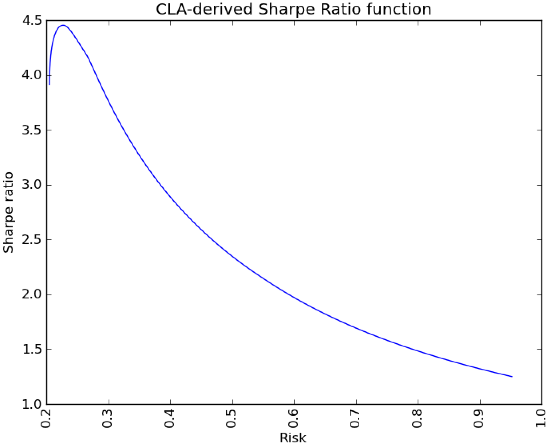
4.2. Search for the Maximum Sharpe Ratio Portfolio

The turning point with the maximum Sharpe ratio does not necessarily coincide with the maximum Sharpe ratio portfolio. Although we have not explicitly computed the maximum Sharpe ratio portfolio yet, we have the building blocks needed to construct it. Every two neighbor turning points define a segment of the efficient frontier. The weights that form each segment result from the convex combination of the turning points at its edges.

For $\alpha \in \left[0,1\right]$, $\omega =\alpha {\omega }_0+\left(1-\alpha \right){\omega }_1$ gives the portfolios associated with the segment of the efficient frontier delimited by ${\omega }_0$ and ${\omega }_1$. The Sharpe ratio is a strongly unimodal function of $\lambda$ (see [15] for a proof). We know that $\lambda$ is a strictly monotonic function of $\alpha$, because $\lambda$ cannot increase as we transition from ${\omega }_0$ to ${\omega }_1$. The conclusion is that the Sharpe ratio function is also a strongly unimodal function of $\alpha$. This means that we can use the Golden Section algorithm to find the maximum Sharpe ratio portfolio within the appropriate segment (The Golden Section search is a numerical algorithm for finding the minimum or maximum of a real-valued and strictly unimodal function. This is accomplished by sequentially narrowing the range of values inside which the minimum or maximum exists. Avriel [16] introduced this technique, and [17] proved its optimality). Snippet 13 shows an implementation of such algorithm. The goldenSection function receives as arguments:

• obj: The objective function on which the extreme will be found.
• a: The leftmost extreme of search.
• b: The rightmost extreme of search.
• **kargs: Keyworded variable-length argument list.

Snippet 13. Golden section search algorithm.

def goldenSection(self, obj, a, b, **kargs):

  # Golden section method. Maximum if kargs['minimum'] == False is passed

  from math import log,ceil

  tol, sign, args = 1.0e −9, 1, None

  if 'minimum' in kargs and kargs['minimum'] == False:sign = −1

  if 'args' in kargs:args = kargs['args']

  numIter = int(ceil(−2.078087*log(tol/abs(b − a))))

  r = 0.618033989

  c = 1.0 − r

  # Initialize

  x1 = r*a + c*b; x2 = c*a + r*b

  f1 = sign*obj(x1, *args); f2 = sign*obj(x2, *args)

  # Loop

  for i in range(numIter):

   if f1 > f2:

    a = x1

    x1 = x2; f1 = f2

    x2 = c*a + r*b; f2 = sign*obj(x2, *args)

   else:

    b = x2

    x2 = x1; f2 = f1

    x1 = r*a + c*b; f1 = sign*obj(x1, *args)

  if f1 < f2:return x1, sign*f1

  else:return x2, sign*f2

The extremes of the search are delimited by the neighbor turning points, which we pass as a keyworded variable length argument (kargs). kargs is a dictionary composed of two optional arguments: “minimum” and “args”. Our implementation of the Golden Section algorithm searches for a minimum by default, however it will search for a maximum when the user passes the optional argument “minimum” with value False. “args” contains a non-keyworded variable-length argument, which (if present) is passed to the objective function obj. This approach allows us to pass as many arguments as the objective function obj may need in other applications. Note that, for this particular utility, we have imported two additional functions from Python’s math library: log and ceil.

We ignore which segment contains the portfolio that delivers the global maximum Sharpe ratio. We will compute the local maximum of the Sharpe ratio function for each segment, and store the output. Then, the global maximum will be determined by comparing those local optima. This operation is conducted by the function getMaxSR in Snippet 14. evalSR is the objective function (obj) which we pass to the goldenSection routine, in order to evaluate the Sharpe ratio at various steps between ${\omega }_0$ and ${\omega }_1$. We are searching for a maximum between those two turning points, and so we set kargs = {'minimum':False, 'args':(w0, w1)}.

Snippet 14. The search for Maximum Sharpe ratio portfolio.

def getMaxSR(self):

  # Get the max Sharpe ratio portfolio

  #1) Compute the local max SR portfolio between any two neighbor turning points

  w_sr, sr = [], []

  for i in range(len(self.w) − 1):

   w0 = np.copy(self.w[i])

   w1 = np.copy(self.w[i + 1])

   kargs = {'minimum':False, 'args':(w0, w1)}

   a, b = self.goldenSection(self.evalSR, 0, 1, **kargs)

   w_sr.append(a*w0 + (1 − a)*w1)

   sr.append(b)

  return max(sr), w_sr[sr.index(max(sr))]

#---------------------------------------------------------------

def evalSR(self, a, w0, w1):

  # Evaluate SR of the portfolio within the convex combination

  w = a*w0 + (1 − a)*w1

  b = np.dot(w.T, self.mean)[0,0]

  c = np.dot(np.dot(w.T, self.covar), w)[0,0]**.5

  return b/c

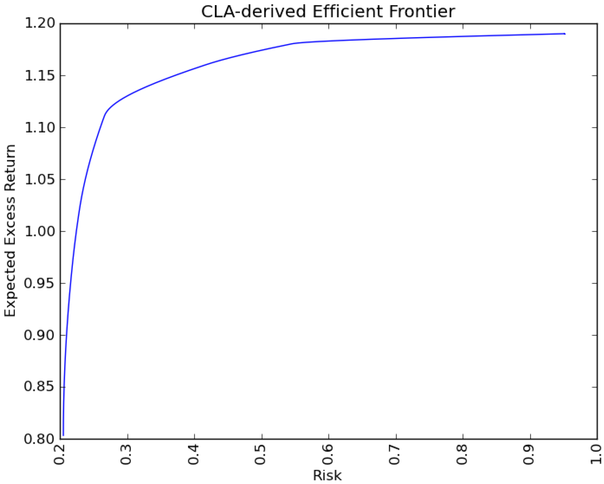
4.3. Computing the Efficient Frontier

As argued earlier, we can compute the various segments of the efficient frontier as a convex combination between any two neighbor turning points. This calculation is carried out by the function efFrontier in Snippet 15. We use the Numpy function linspace to uniformly partition the unit segment, excluding the value 1. The reason for this exclusion is, the end of one convex combination coincides with the beginning of another, and so the uniform partition should contain that value 0 or 1, but not both. When we reach the final pair of turning points, we include the value 1 in the uniform partition, because this is the last iteration and the resulting portfolio will not be redundant. efFrontier outputs three lists: Means, Standard Deviations and the associated portfolio weights. The number of items in each of these lists is determined by the argument points.

Snippet 15. Computing the Efficient Frontier.

def efFrontier(self, points):

  # Get the efficient frontier

  mu, sigma, weights = [], [], []

  a = np.linspace(0, 1, points/len(self.w))[:−1] # remove the 1, to avoid duplications

  b = range(len(self.w) − 1)

  for i in b:

   w0, w1 = self.w[i], self.w[i + 1]

   if i == b[−1]:a = np.linspace(0, 1, points/len(self.w)) # include the 1 in the last iteration

   for j in a:

    w = w1*j + (1 − j)*w0

    weights.append(np.copy(w))

    mu.append(np.dot(w.T, self.mean)[0, 0])

    sigma.append(np.dot(np.dot(w.T, self.covar), w)[0, 0]**.5)

  return mu, sigma, weights

5. A Numerical Example

We will run our Python implementation of CLA on the same example that accompanies the VBA-Excel implementation by [6]. Table 1 provides the vector of expected returns and the covariance matrix of returns. We set as boundary conditions that $0\le {\omega }_i\le 1, \forall i=1,\dots ,n$, and the implicit condition that $\sum _{i=1}^n{\omega }_i=1$.

Table 1. Covariance Matrix, Vector of Expected Returns and boundary conditions.

L Bound	0	0	0	0	0	0	0	0	0	0
U Bound	1	1	1	1	1	1	1	1	1	1
Mean	1.175	1.19	0.396	1.12	0.346	0.679	0.089	0.73	0.481	1.08
Cov	0.4075516
	0.0317584	0.9063047
	0.0518392	0.0313639	0.194909
	0.056639	0.0268726	0.0440849	0.1952847
	0.0330226	0.0191717	0.0300677	0.0277735	0.3405911
	0.0082778	0.0093438	0.0132274	0.0052667	0.0077706	0.1598387
	0.0216594	0.0249504	0.0352597	0.0137581	0.0206784	0.0210558	0.6805671
	0.0133242	0.0076104	0.0115493	0.0078088	0.0073641	0.0051869	0.0137788	0.9552692
	0.0343476	0.0287487	0.0427563	0.0291418	0.0254266	0.0172374	0.0462703	0.0106553	0.3168158
	0.022499	0.0133687	0.020573	0.0164038	0.0128408	0.0072378	0.0192609	0.0076096	0.0185432	0.1107929

Table 1. Covariance Matrix, Vector of Expected Returns and boundary conditions.

L Bound	0	0	0	0	0	0	0	0	0	0
U Bound	1	1	1	1	1	1	1	1	1	1
Mean	1.175	1.19	0.396	1.12	0.346	0.679	0.089	0.73	0.481	1.08
Cov	0.4075516
	0.0317584	0.9063047
	0.0518392	0.0313639	0.194909
	0.056639	0.0268726	0.0440849	0.1952847
	0.0330226	0.0191717	0.0300677	0.0277735	0.3405911
	0.0082778	0.0093438	0.0132274	0.0052667	0.0077706	0.1598387
	0.0216594	0.0249504	0.0352597	0.0137581	0.0206784	0.0210558	0.6805671
	0.0133242	0.0076104	0.0115493	0.0078088	0.0073641	0.0051869	0.0137788	0.9552692
	0.0343476	0.0287487	0.0427563	0.0291418	0.0254266	0.0172374	0.0462703	0.0106553	0.3168158
	0.022499	0.0133687	0.020573	0.0164038	0.0128408	0.0072378	0.0192609	0.0076096	0.0185432	0.1107929

Snippet 16 shows a simple example of how to use the CLA class. We have stored the data in a csv file, with the following structure:

• Row 1: Headers
• Row 2: Mean vector
• Row 3: Lower bounds
• Row 4: Upper bounds
• Row 5 and successive: Covariance matrix

Snippet 16. Using the CLA class.

def main():

 import numpy as np

 import CLA

 #1) Path

 path='H:/PROJECTS/Data/CLA_Data.csv'

 #2) Load data, set seed

 headers=open(path,'r').readline().split(',')[:-1]

 data=np.genfromtxt(path,delimiter=',',skip_header=1) # load as numpy array

 mean=np.array(data[:1]).T

 lB=np.array(data[1:2]).T

 uB=np.array(data[2:3]).T

 covar=np.array(data[3:])

  #3) Invoke object

 cla=CLA.CLA(mean,covar,lB,uB)

 cla.solve()

 print cla.w # print all turning points

 #4) Plot frontier

 mu,sigma,weights=cla.efFrontier(100)

 plot2D(sigma, mu, 'Risk', 'Expected Excess Return', 'CLA-derived Efficient Frontier')

 #5) Get Maximum Sharpe ratio portfolio

 sr,w_sr = cla.getMaxSR()

 print np.dot(np.dot(w_sr.T, cla.covar), w_sr)[0, 0]**.5, sr

 print w_sr

 #6) Get Minimum Variance portfolio

 mv, w_mv = cla.getMinVar()

 print mv

 print w_mv

 return

#---------------------------------------------------------------

# Boilerplate

if __name__ == '__main__':main()

The key lines of code are:

• cla = CLA.CLA(mean, covar, lB, uB): This creates a CLA object named cla, with the input parameters read from the csv file.
• cla.solve(): This runs the solve method within the CLA class (see the Appendix), which comprises all the Snippets listed in Section 3 (Snippets 1–11).

Once the cla.solve() method has been run, results can be accessed easily:

• cla.w contains a list of all turning points.
• cla.l and cla.g respectively contain the values of $\lambda$ and $\gamma$ for every turning point.
• cla.f contains the composition of F used to compute every turning point.

Table 2 reports these outputs for our particular example. Note that sometimes an asset may become free, and yet the turning point has the weight for that asset resting precisely at the same boundary it became free from. In that case, the solution may seem repeated, when in fact what is happening is that the same portfolio is the result of two different F sets.

Table 2. Return, Risk, λ and composition of the 10 turning points.

CP Num	Return	Risk	Lambda	X(1)	X(2)	X(3)	X(4)	X(5)	X(6)	X(7)	X(8)	X(9)	X(10)
1	1.190	0.952	58.303	0.000	1.000	0.000	0.000	0.000	0.000	0.000	0.000	0.000	0.000
2	1.180	0.546	4.174	0.649	0.351	0.000	0.000	0.000	0.000	0.000	0.000	0.000	0.000
3	1.160	0.417	1.946	0.434	0.231	0.000	0.335	0.000	0.000	0.000	0.000	0.000	0.000
4	1.111	0.267	0.165	0.127	0.072	0.000	0.281	0.000	0.000	0.000	0.000	0.000	0.520
5	1.108	0.265	0.147	0.123	0.070	0.000	0.279	0.000	0.000	0.000	0.006	0.000	0.521
6	1.022	0.230	0.056	0.087	0.050	0.000	0.224	0.000	0.174	0.000	0.030	0.000	0.435
7	1.015	0.228	0.052	0.085	0.049	0.000	0.220	0.000	0.180	0.000	0.031	0.006	0.429
8	0.973	0.220	0.037	0.074	0.044	0.000	0.199	0.026	0.198	0.000	0.033	0.028	0.398
9	0.950	0.216	0.031	0.068	0.041	0.015	0.188	0.034	0.202	0.000	0.034	0.034	0.383
10	0.803	0.205	0.000	0.037	0.027	0.095	0.126	0.077	0.219	0.030	0.036	0.061	0.292

Table 2. Return, Risk, λ and composition of the 10 turning points.

CP Num	Return	Risk	Lambda	X(1)	X(2)	X(3)	X(4)	X(5)	X(6)	X(7)	X(8)	X(9)	X(10)
1	1.190	0.952	58.303	0.000	1.000	0.000	0.000	0.000	0.000	0.000	0.000	0.000	0.000
2	1.180	0.546	4.174	0.649	0.351	0.000	0.000	0.000	0.000	0.000	0.000	0.000	0.000
3	1.160	0.417	1.946	0.434	0.231	0.000	0.335	0.000	0.000	0.000	0.000	0.000	0.000
4	1.111	0.267	0.165	0.127	0.072	0.000	0.281	0.000	0.000	0.000	0.000	0.000	0.520
5	1.108	0.265	0.147	0.123	0.070	0.000	0.279	0.000	0.000	0.000	0.006	0.000	0.521
6	1.022	0.230	0.056	0.087	0.050	0.000	0.224	0.000	0.174	0.000	0.030	0.000	0.435
7	1.015	0.228	0.052	0.085	0.049	0.000	0.220	0.000	0.180	0.000	0.031	0.006	0.429
8	0.973	0.220	0.037	0.074	0.044	0.000	0.199	0.026	0.198	0.000	0.033	0.028	0.398
9	0.950	0.216	0.031	0.068	0.041	0.015	0.188	0.034	0.202	0.000	0.034	0.034	0.383
10	0.803	0.205	0.000	0.037	0.027	0.095	0.126	0.077	0.219	0.030	0.036	0.061	0.292

We can also access the utilities described in Section 4. For instance, the instruction mu, sigma, weights = cla.efFrontier(100) in Snippet 16 computes 100 points of the Efficient Frontier, and plots them using the auxiliary function in Snippet 17. If the optional argument pathChart is not used, the chart is plotted, but if a path is provided, the chart is saved as a file in that destination.

Snippet 17. The efficient frontier.

def plot2D(x, y, xLabel = '', yLabel = '', title = '', pathChart = None):

 import matplotlib.pyplot as mpl

 fig = mpl.figure()

 ax = fig.add_subplot(1, 1, 1) # one row, one column, first plot

 ax.plot(x, y, color = 'blue')

 ax.set_xlabel(xLabel)

 ax.set_ylabel(yLabel, rotation = 90)

 mpl.xticks(rotation = 'vertical')

 mpl.title(title)

 if pathChart == None:

  mpl.show()

 else:

  mpl.savefig(pathChart)

 mpl.clf() # reset pylab

 return

Figure 1 plots the efficient frontier, using the plot2D function provided in Snippet 17. Figure 2 plots the Sharpe ratio as a function of risk. Visually, the maximum Sharpe ratio portfolio is located around a risk of 0.2, and reaches a level close to 4.5. This can be easily verified by running the instruction sr, w_sr = cla.getMaxSR(), which returns a Sharpe ratio of 4.4535 for a portfolio with risk 0.2274. Similarly, running the instruction mv, w_mv = cla.getMinVar() reports a Minimum Variance portfolio with a risk of 0.2052.

Figure 1. The Efficient Frontier

Figure 1. The Efficient Frontier

Figure 2. Sharpe ratio as a function of risk.

Figure 2. Sharpe ratio as a function of risk.

VBA-Excel’s double data type is based on a modified IEEE 754 specification, which offers a precision of 15 significant figures ([18]). Our Python results exactly match the outputs obtained when using the implementation of [6], to the highest accuracy offered by VBA-Excel.

6. Conclusions

Portfolio optimization is one of the problems most frequently encountered by financial practitioners. Following Markowitz [1], this operation consists in identifying the combination of assets that maximize the expected return subject to a certain risk budget. For a complete range of risk budgets, this gives rise to the concept of Efficient Frontier. This problem has an analytical solution in the absence of inequality constraints, such as lower and upper bounds for portfolio weights.

In order to cope with inequality constraints, [3,4] introduced the Critical Line Algorithm (CLA). To our knowledge, CLA is the only algorithm specifically designed for linear inequality-constrained quadratic portfolio optimization problems, which guarantees that the exact solution is found after a given number of iterations. Furthermore, CLA does not only compute a single portfolio, but it derives the entire efficient frontier. In the context of portfolio optimization problems, this approach is clearly more adequate than generic-purpose quadratic programming algorithms.

Given these two facts that portfolio optimization is a critical task, and that CLA provides an extremely efficient solution method, one would expect a myriad of software implementations to be available. Yet, to our surprise, we are only aware of one open-source, fully documented implementation of CLA, by [6]. Unfortunately, that implementation was done in VBA-Excel. This requires manual adjustments to a spreadsheet, which inevitably narrows its applicability to small-scale problems. Consequently, we suspect that most financial practitioners are resorting to generic-purpose quadratic programming software to optimize their portfolios, which often delivers suboptimal solutions.

The main goal of this paper is to fill this gap in the literature by providing a well-documented, step-by-step open-source implementation of CLA in a scientific language. The code is implemented as a Python class object, which allows it to be imported like any other Python module, and integrated seamlessly with pre-existing code. Following the explanation provided in this paper, our class can also be easily translated to other languages, such as C, C++ or Fortran-90. We have discussed the logic behind CLA following the algorithm’s decision flow. In addition, we have developed several utilities that facilitate the answering of recurrent practical problems. Our results match the output of [6] at the highest accuracy offered by Excel.

References

1. Markowitz, H.M. Portfolio selection. J. Financ. 1952, 7, 77–91. [Google Scholar]
2. Beardsley, B.; Donnadieu, H.; Kramer, K.; Kumar, M.; Maguire, A.; Morel, P.; Tang, T. Capturing Growth in Adverse Times: Global Asset Management 2012. Research Paper, The Boston Consulting Group, Boston, MA, USA, 2012. [Google Scholar]
3. Markowitz, H.M. The optimization of a quadratic function subject to linear constraints. Nav. Res. Logist. Q. 1956, 3, 111–133. [Google Scholar] [CrossRef]
4. Markowitz, H.M. Portfolio Selection: Efficient Diversification of Investments, 1st ed.; John Wiley and Sons: New York, NY, USA, 1959. [Google Scholar]
5. Wolfe, P. The simplex method for quadratic programming. Econometrica 1959, 27, 382–398. [Google Scholar] [CrossRef]
6. Markowitz, H.M.; Todd, G.P. Mean Variance Analysis in Portfolio Choice and Capital Markets, 1st ed.; John Wiley and Sons: New York, NY, USA, 2000. [Google Scholar]
7. Markowitz, H.M.; Malhotra, A.; Pazel, D.P. The EAS-E application development system: principles and language summary. Commun. ACM 1984, 27, 785–799. [Google Scholar] [CrossRef]
8. Steuer, R.E.; Qi, Y.; Hirschberger, M. Portfolio optimization: New capabilities and future methods. Z. Betriebswirtschaft 2006, 76, 199–219. [Google Scholar] [CrossRef]
9. Kwak, J. The importance of Excel. The Baseline Scenario, 9 February 2013. Available online: http://baselinescenario.com/2013/02/09/the-importance-of-excel/ (accessed on 21 March 2013).
10. Hirschberger, M.; Qi, Y.; Steuer, R.E. Quadratic Parametric Programming for Portfolio Selection with Random Problem Generation and Computational Experience. Working Paper, Terry College of Business, University of Georgia, Athens, GA, USA, 2004. [Google Scholar]
11. Niedermayer, A.; Niedermayer, D. Applying Markowitz’s Critical Line Algorithm. Research Paper Series, Department of Economics, University of Bern, Bern, Switzerland, 2007. [Google Scholar]
12. Black, F.; Litterman, R. Global portfolio optimization. Financ. Anal. J. 1992, 48, 28–43. [Google Scholar] [CrossRef]
13. Bailey, D.H.; López de Prado, M. The sharpe ratio efficient frontier. J. Risk 2012, 15, 3–44. [Google Scholar] [CrossRef]
14. Meucci, A. Risk and Asset Allocation, 1st ed.; Springer: New York, NY, USA, 2005. [Google Scholar]
15. Kopman, L.; Liu, S. Maximizing the Sharpe Ratio. MSCI Barra Research Paper No. 2009-22. MSCI Barra: New York, NY, USA, 2009. [Google Scholar]
16. Avriel, M.; Wilde, D. Optimality proof for the symmetric Fibonacci search technique. Fibonacci Q. 1966, 4, 265–269. [Google Scholar]
17. Dalton, S. Financial Applications Using Excel Add-in Development in C/C++, 2nd ed.; John Wiley and Sons: New York, NY, USA, 2007; pp. 13–14. [Google Scholar]
18. Kiefer, J. Sequential minimax search for a maximum. Proc. Am. Math. Soc. 1953, 4, 502–506. [Google Scholar] [CrossRef]
19. David, H. Bailey’s Research Website. Available online: www.davidhbailey.com (accessed on 21 March 2013).
20. Marcos López de Prado’s Research Website. Available online: www.quantresearch.info (accessed on 21 March 2013).