1. Introduction
Discerning the major components of a point cloud is of importance for finding patterns in the cloud and for compressing it. Principal Component Analysis (PCA) is a widely used successful tool to determine the direction, spread, and dimensionality of point clouds [
1,
2]). In its standard formulation, PCA is based on analysis in the square of the
norm applicable to data from distributions with finite second-order moments. This results in excellent performance when the point cloud has Gaussian structure or the structure of a distribution close to Gaussian. However, point clouds obtained under conditions other than benign laboratory conditions often contain significant numbers of outliers and the points may follow a heavy-tailed distribution that does not have finite second-order moments, which strongly limits the accuracy of standard PCA or prevents it from being applicable.
To remedy this situation, robust PCAs [
3,
4,
5,
6] and especially robust PCAs involving the
norm [
7,
8,
9,
10] have been investigated over the past few years. In most of the
reformulations of PCA that have been proposed, the
norm is applied only to parts of the PCA process. An analytical connection with heavy-tailed statistics is not present in any of these reformulations. Much of the previous work on
methods for PCA and in other areas has been carried out under the assumption of sparsity of the principal components or of the error. But the principal components and the error are often not sparse. While an assumption of sparsity is common in many areas (for example, in compressed sensing) and can lead to meaningful analytical and computational results in those areas, it restricts the set of situations that a reformulated PCA can address. Finally, neither standard PCA nor any of the reformulated robust PCAs are able to provide reliable information for distributions with two or more irregularly spaced main directions (spokes, such as from superimposing several classical distributions).
We hypothesize that
-based concepts such as singular values, inner products, orthogonal projection, averaging and second-order moments (variances and covariances) in the reformulated PCAs that have been investigated in the recent literature are limiting factors in the applicability of these PCAs to realistic outlier-rich point clouds that occur in geometric modeling, image analysis, object and face recognition, data mining, network analysis and many other areas. To remedy this situation, we carry out here a fundamental reformulation of the PCA approach in a framework based not just in part but in total on the
norm. The
norm is chosen because it is an appropriate norm when the data cloud has a significant number of outliers, either artificial outliers or outliers of a heavy-tailed statistical distribution. While analysis of multivariate heavy-tailed distributions is still underdeveloped, there has been progress [
11,
12,
13,
14]). Our
approach here is related to the approach by which
splines, a new class of splines that preserve shape for highly irregular data, have been created over the past 12 years [
15,
16,
17,
18,
19].
2. Standard PCA and Recently Developed Robust PCAs
In its standard formulation [
2], PCA is designed to create uncorrelated components (“orthogonal solutions”). There are variants of PCA that create correlated components (“oblique solutions”), but we do not consider them here. Principal components are normally calculated using the singular value decomposition of the data matrix, an efficient and stable numerical procedure. Standard PCA can be summarized as follows:
Calculate the mean of the point cloud and subtract it out of the data.
Set up the matrix X of the data that result from Step 1. The rows of X are the data vectors.
Calculate the singular values of X, that is, the diagonal elements of the matrix Σ in the singular value decomposition . (These singular values are the eigenvalues of the covariance matrix of the data.)
Order the components (the columns of the matrix V in the singular value decomposition) in descending order of the singular values.
Select basis vectors to be the components corresponding to the largest singular values.
Conduct further processing (for example, project the data onto the basis consisting of the vectors selected in Step 5).
Step 3 makes the limitations of standard PCA apparent. For the singular values to be meaningful, the covariance matrix of the continuum distribution from which the samples come needs to exist, that is, be finite. There are heavy-tailed distributions for which covariance matrices exist and others for which they do not. When there are a significant number of outliers in the data, an assertion that the covariance matrix of the continuum distribution exists can be dubious. A large number of outliers in the data is often an indication that the data come from a continuum heavy-tailed distribution for which the covariance matrix may not exist (has infinite entries). While the covariance matrix of a finite sample always exists, it is meaningful only if the covariance matrix of the underlying continuum distribution exists. In the remainder of this section, we discuss four robust variants of PCA that are currently in use.
Candès
et al. [
7] use the “nuclear norm” of a matrix in their robust PCA. The nuclear norm of a matrix
P, denoted by
, is the sum of the singular values of
P. Let
denote the sum of the absolute values of the entries of a matrix
E. Let
D be the data matrix,
P be the matrix of principal components, and
E be the error matrix. Candès
et al. formulate the robust PCA problem as minimization of
under assumptions that
P is of low rank and
E is sparse. Here,
λ is a prescribed parameter based on the size of the data set [
7]. Using an
norm to replace an
norm in a computational method is often a good procedure for robustifying the method. Minimization of expression (
1) is seemingly based on the
norm, since both of the norms that occur in the objective-functional portion of expression (1) consist of sums of absolute values. However, the nuclear norm is not an
metric but only a “pseudo-
” metric because the singular values on which it is based are created by an
-based process. Moreover, the arithmetic mean used to center the data is also an
, not an
quantity. It is our hypothesis that a procedure that avoids use of singular values, which are
quantities, and is based completely on the
metric will provide more accurate output information about realistic outlier-rich data than robust PCAs that are based on the use of singular values.
Kwak [
10] proposes maximizing the
norm of the product of a vector and the data matrix and provides face recognition results that indicate success. This method uses inner products (a matrix or a vector times a matrix), which are
operations that do not exist in an
space. Here again, we surmise that a procedure that avoids use of all
quantities and is based completely on the
metric will have better performance.
Croux and Ruiz-Gazen [
4] calculate robust estimates of the eigenvalues and eigenvectors of the covariance matrix without estimating the covariance matrix itself. Their method is based on a projection-pursuit approach developed by Li and Chen [
20]. In this approach, one searches for directions for which the data, projected onto these directions, have maximal dispersion. This dispersion is measured not by the variance but by a robust scale estimator
. For data
, the estimate of the first eigenvector is defined to be
and the associated eigenvalue is
Subsequent eigenvectors are determined by searching in an analogous manner over subspaces orthogonal to all subspaces already found. Croux and Ruiz-Gazen [
4] made the projection-pursuit process of Li and Chen more efficient by approximating on each step a full-space search for the vector
a by a search over a finite set while retaining a high finite-sample breakdown point.
Finally, Ke and Kanade [
8,
9] seek a
factorization of the data matrix
such that
is minimized. This method uses the
norm but also involves
inner products (matrix multiplication). The minimization of expression (
4) is non-convex, so Ke and Kanade calculate
U and
V iteratively with a random initialization of
U, optimizing one matrix while keeping the other one fixed, in the following manner. Given
,
is defined to be
The next
U, that is,
is defined to be
These two
minimization problems can be decomposed into independent minimization problems that Ke and Kanade solve by linear programming or, approximately, by quadratic programming.
In addition to the issues mentioned above, currently available robust PCAs are not able to meaningfully handle data from distributions with multiple, irregularly spaced main directions or “spokes,” that is, directions in which the level surfaces of the probability density function extend further out from the central point than in neighboring directions, a situation that is increasingly common for some physical and a lot of non-physical (sociological, cognitive, human-behavior,
etc.) data. These PCAs provide only one main direction that accounts for the largest variability in the data and additional orthogonal directions that account for the remaining variability. But these directions may provide very little information about the data. In the literature, one extension of PCA that detects orthogonal spokes using a union-of-subspaces model is available [
21]. However, this extension does not involve the
norm and is therefore not robust when a significant number of outliers is present. It is possible that “superstructure” could be added to standard PCA and to robust PCAs to allow them to calculate multiple non-orthogonal spokes, but such generalizations of these methods are not yet available in the literature. There is nevertheless a need to develop a method that can calculate the directions and spreads of multiple major components.
In the next section, we consider how to reformulate the PCA approach in a framework based exclusively on the norm and heavy-tailed distributions, without using any -based concepts, in a way that allows calculation of the directions and spreads of single and of multiple major components. Our reformulation occurs in a manner that differs from previous -based robust PCAs not merely in algorithmic structure but also in theory. The theory that we propose relies on the linkage between heavy-tailed distributions and the norm, a linkage that is not discussed in the previous literature about robust PCAs.
3. 2D Major Component Detection and Analysis
Reformulation of the PCA approach in the
norm involves more than adjusting individual steps in the standard PCA process that was outlined in
Section 2. One must now accomplish the objective of determining the main directions and the magnitudes of the spread of the point cloud in those directions without the tools (singular values, inner products, orthogonal projection, averaging and second-order moments) of the standard
-based approach.
The
Major Component Detection and Analysis (
MCDA) that we propose consists of the following two steps:
Calculate the central point of the data and subtract it out of the data.
Calculate the main directions of the point cloud that results from Step 1 and the magnitudes of radial extension in those directions.
Post-processing analogous to Step 6 of standard PCA will be part of a fully developed
MCDA in the future but will not be discussed in this paper.
The point cloud under consideration is denoted by
. The distance between points
x and
y in the data space is denoted by
. Since the
norm requires fewer operations than the
norm (see Remark 1 below), we will use the
norm to define the distance function in the data space for the description of the algorithm in the present section and for the computational experiments discussed in
Section 4. However,
MCDA works with any distance function in the data space that the user wishes to choose, for example, the
norm. The distance function does need not to satisfy the triangle inequality but does need to allow definition of angular coordinates. All
norms,
, allow definition of angular coordinates. We do not require orthogonality of the main directions of the distribution but do allow orthogonality to be imposed based on outside information, for example, when we wish to identify major components of a point cloud that is known to be from a distribution with orthogonal main directions or when the data are geometric data with orthogonal main directions in a Euclidean space.
Remark 1 Minimization of a “linear” functional (sum of absolute values of linear components) is a linear programming problem that is generally more expensive to solve than minimization of a corresponding functional (sum of squares of linear components), which is carried out by solving one linear system. Not surprisingly, therefore, the MCDA that we will develop will be more expensive than standard -based PCA. However, as a functional for measuring distance in the data space, the norm is not an minimization problem but rather simply a defined metric. As a metric in the data space, the norm, which is a sum of absolute values, is computationally much cheaper than the norm, which is a square root of a sum of products. Rotation in -normed space consists of adding and/or subtracting quantities from the coordinates while rotation in -normed space involves the more expensive operations of calculation of multiple sums of products. This situation suggests that using the norm in the data space is meaningful. Even when the natural norm in the data space is the norm, using the computationally cheaper norm as an approximation of the norm (rather than vice versa as has traditionally been the case) is a meaningful choice. The fact that -based methods are more expensive than -based methods in many higher-level situations does not change the fact that the metric is much less expensive than the metric at the lowest level of measuring distance in a data space.
3.1. MCDA Step 1: Calculation of the Central Point
We define the multivariate median to be the point
that minimizes
In standard PCA, the central point is calculated by minimizing (
7) with the square of the
norm as the distance function
d. This yields the multidimensional average, which costs
(sequential) operations. However, many heavy-tailed distributions, including the Student
t distribution with 1 degree of freedom that we will use in the computational experiments in this paper, do not have an average. When the continuum distribution from which a sample is drawn does not have an average, using the average of the data points in that sample for any purpose whatsoever is wrong. When
d is the
norm,
is the coordinate-wise median, an estimator of the central point [
22], that consists of scalar medians (one for each coordinate direction) and costs
(sequential). In this paper, we will use the coordinate-wise median, which exists for all heavy-tailed and light-tailed distributions, as the central point of the data set.
Remark 2 For distributions with spokes that are not symmetrically positioned around a central point, the coordinate-wise median is not an appropriate central point. Other options such as the “
-median” investigated by Fritz
et al. [
23] in which the distance function
d is the
norm (rather than the widely chosen square of the
norm square of the
norm) may be more meaningful. In the present paper, we will assume that all of the spokes of the data are symmetrically positioned around a central point, that opposite spokes have the same structure and, therefore, that the coordinate-wise median is an appropriate central point.
Once the central point is calculated, it is subtracted out of the data, resulting in a point cloud that is centered at the origin of the space. Since there is little possibility of confusion, we denote the data set after the central point has been subtracted out by , the same notation used for the original data set.
3.2. MCDA Step 2: Calculation of the Main Directions
After the data have been centered in Step 1, we need to calculate the main directions in which the distribution extends. Standard PCA prescribes that the main directions of the distribution are orthogonal to each other and that the measure of the extension in each of the orthogonal directions is determined by the covariance matrix. Such structure is consistent with a standard assumption of Gaussian or near-Gaussian distribution of the data. This structure is a leading factor in keeping the computational cost of standard PCA (calculated by singular value decomposition) low. At the same time, its rigidity is a cause of the limited applicability of standard PCA.
The central point of a symmetric univariate heavy-tailed distribution is its 50% quantile, the median of the distribution. The spread of a univariate heavy-tailed distribution around its central point is represented by the distance to other quantiles, for example, the 25% and 75% quantiles. The further away the 25% and 75% quantiles are from the central point, the more spread out (flatter, with heavier tails) the distribution is. One can calculate the 25% and 75% quantiles by calculating the median of the data between the 0% quantile and 50% quantile and the median of the data between the 50% quantile and 100% quantile, respectively. This procedure for calculating the 25% and 75% quantiles is used here because it can be generalized to higher dimensions. For symmetric distributions, one need, of course, calculate only the 25% or the 75% quantile, not both. The univariate situation provides the guideline for how we approach determining the properties of a multivariate heavy-tailed distribution. How heavy-tailed a multivariate distribution is in a given direction is estimated by the “median radius” of the data points in and near that direction.
Assume for now that, as previously stated, the distribution is symmetric around the origin, that is, “spokes” are in precisely opposite directions. Since the distribution is symmetric, we map, without loss of generality, every original data point
for which
or for which
and
to an origin-symmetric data point
. To avoid proliferation of notation, we denote each such data point
also by
. For each data point
(whether an original data point or a data point obtained by mapping to the origin-symmetric point), define the
direction
(analogous to an angle in
polar coordinates) to be the
y-coordinate of the corresponding point on the
“unit circle” (unit diamond), that is,
Here, all of the coordinates
are nonnegative and the
are in the interval
. In what follows, we will need periodic extension of the
’s. Let
for some integer
s and for
m,
. The
for
k outside the range
are defined in a natural manner as
(This situation is a direct analogue of the fact that the standard
angle
α of a point can be represented by
for any integer
s.) The original data points as well as the data points obtained in this manner can be represented in “polar” form as
where
is the
radius of the data point.
In what follows, we assume that the data points have been ordered so that the values of increase monotonically with m. To avoid proliferation of notation, we use the same notation for the sorted data that was used for the unsorted data.
Due to statistical variability, we cannot find good approximations of the directions in which the distribution spreads farthest simply by identifying the locally largest values of
(as a function of
m). One estimates the directions in which the multidimensional distribution spreads farthest and the extent to which it spreads in these directions by calculating the local maxima with respect to
θ of the median radius of the distribution. To find the directions in which the median radius is locally maximal, we have to approximate the data
in a smooth manner and then find the directions
θ in which this approximation is locally maximal. A method for finding local maxima that relies on fitting the data with a global function would be computationally feasible in 2D. However, fitting a global surface to the data would be less computationally attractive in 3D and 4D (space + time) and not at all computationally useful in
n dimensions for
. For this reason, we adopt the following locally based algorithm for calculating values of a function
that represents the median radius of the data points
and for identifying local maxima of this function:
Choose a point from which to start.
Choose an integer q that represents the number of neighbors in each direction (index lower and higher than m) that will be included in a local domain D.
On the local domain
, calculate the quadratic polynomial
that best fits the data in the
norm, that is, minimizes,
over all real numbers
,
and
.
Determine the location of the maximum of the quadratic polynomial on the local domain D. If the location of the maximum is strictly inside D, go to Step 5. If the location of the maximum is at or , call this direction a new and return to Step 3.
Refine the location and value of the maximum of the median radius in the following way. Calculate a quadratic polynomial on a local domain with a larger around the node closest to the location of the approximate local maximum identified in Step 4. The maximum of this quadratic polynomial is the estimate of the maximum of the median radius.
The above procedure is for calculating one local maximum. To calculate all local maxima for a distribution with several spokes, one needs to assume that the spokes are distinct from each other, that is, do not overlap in a way that two closely placed spokes appear nearly like one spoke. For example, one may have information that the spokes are locally separated by angular distances greater than or equal to a known lower bound. One then chooses starting points for multiple implementations of Step 1 that cover the interval at distances that are slightly less than the lower bound. For applications for which local minima are important, one can calculate local minima analogously.
Remark 3 The (unusual) situation in which all points lie on one or a few radial lines does not allow use of the local fitting method described above and can be taken care of by other procedures. In this case, the maxima of the median radius occur at the directions of the radial lines. From the clusters of points with identical , one identifies the directions of the lines and then calculates the one-dimensional median of the in each cluster.
Theoretical guidance for choosing the q and of Steps 2 and 5 is not yet available but it is clear that q and need to be chosen based on the structure of the distribution and the properties of the outliers in the data. There will certainly be a trade-off between accuracy and computational efficiency. With more noise and outliers, one will need to use larger local domains (more neighbors, that is, larger q and/or ) to retain sufficient accuracy.
4. Computational Experiments
In this section, we present comparisons of 2D
MCDA with standard PCA, Croux and Ruiz-Gazen’s method and Ke and Kanade’s method. Of all the robust PCAs that have been developed, only Ke and Kanade’s method [
8,
9], uses
as its main basis. For this reason, comparison of our
MCDA, which is “fully
”, with Ke and Kanade’s method is important. For further contextual awareness, comparison with another widely used robust PCA, for example, Croux and Ruiz-Gazen’s projection-pursuit method [
4] is equally important.
Eight types of distributions were used for the computational experiments:
Bivariate Gaussian without and with additional artificial outliers
Bivariate Student t with 1 degree of freedom without and with additional artificial outliers
Three superimposed bivariate Gaussians without and with additional artificial outliers
Three superimposed bivariate Student t with 1 degree of freedom without and with additional artificial outliers
Bivariate Student
t distributions with 1 degree of freedom are heavy-tailed distributions with particularly heavy tails. These distributions were chosen for the computational experiments because they represent a significant computational challenge for standard PCA, the robust PCAs and
MCDA.
All computational results were generated by MATLAB R2009b on a sequential 2.50 GHz computer with 1GB memory. The quadratic functions in Steps 3 and 5 of the local
fitting algorithm described in
SubSection 3.2 were calculated by the MATLAB
module. The
q and
of Steps 2 and 5 of the algorithm for calculating the directions and values of the local maxima of the median radius were chosen to be 5 and 12, respectively.
We generated samples from distributions with median radius ρ in the direction α for the following ρ and α. For the one-main-direction situation, we used samples from bivariate distributions with = . Distributions with three main directions were generated by superimposing three distributions with = , and . Samples from the bivariate Student t distributions were generated by the Matlab module using the correlation matrix . These samples were rotated (in ) to the directions mentioned above. In the figures described below in which we illustrate these distributions, we indicate the points of these samples by red dots. Directions and magnitudes of the maxima of the median radius are indicated by bars extending out from the origin.
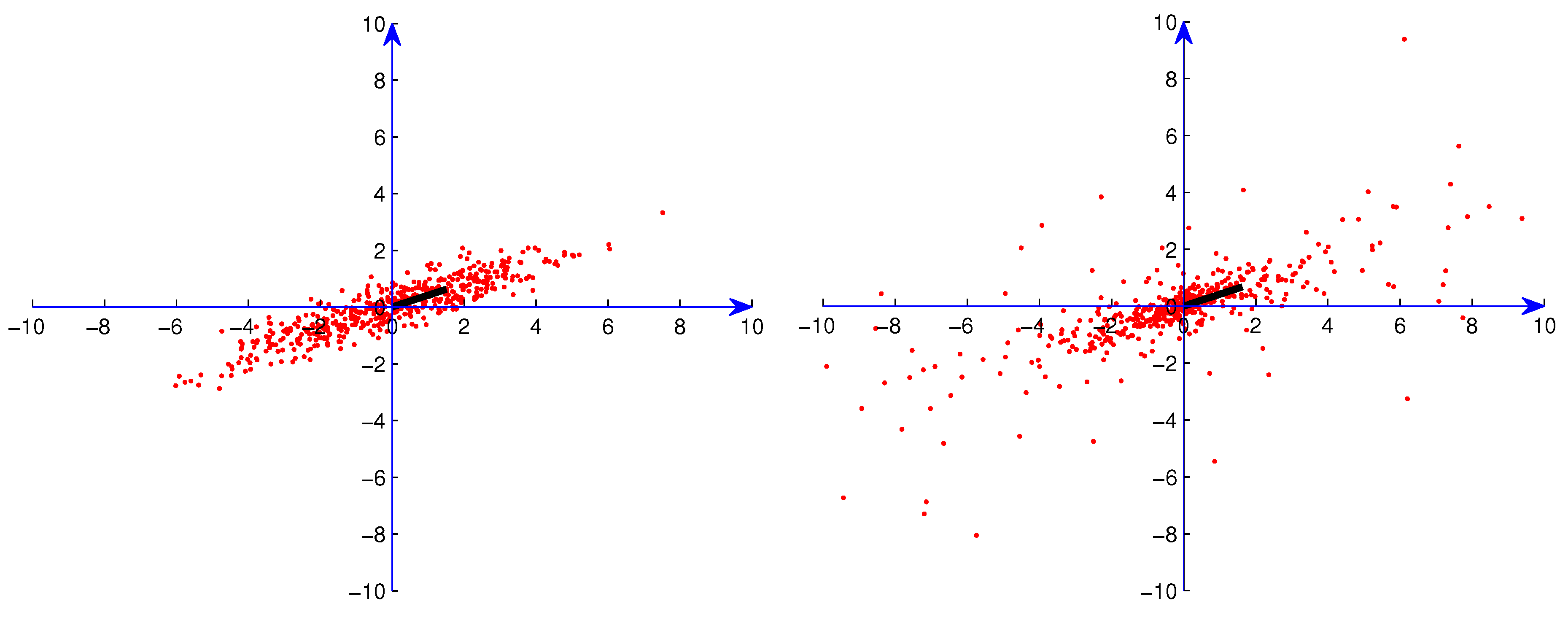
Figure 1.
Sample from one Gaussian distribution without artificial outliers.
Figure 1.
Sample from one Gaussian distribution without artificial outliers.
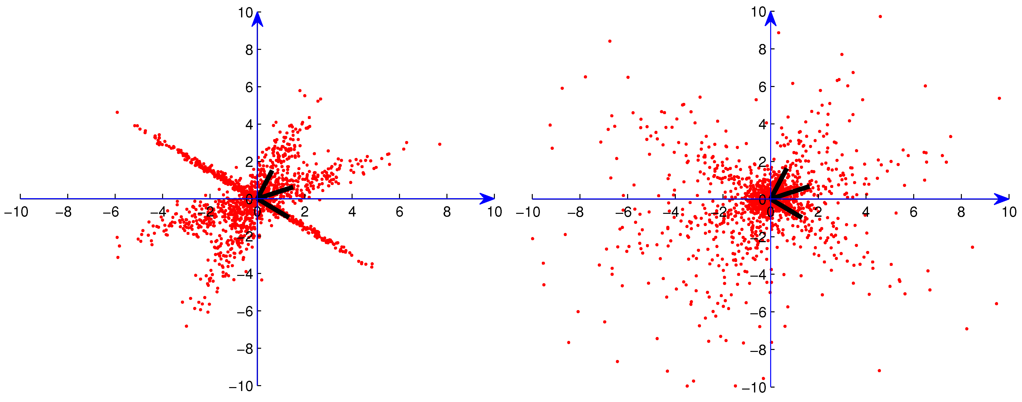
Figure 2.
Sample from three superimposed Gaussian distributions without artificial outliers.
Figure 2.
Sample from three superimposed Gaussian distributions without artificial outliers.
In the computational experiments, we used data sets consisting of 50, 150 and 500 points. In
Figure 1,
Figure 2,
Figure 3 and
Figure 4, we present examples of the data sets with 500 points (red dots) for one Gaussian distribution, one Student
t distribution, three superimposed Gaussian distributions and three superimposed Student
t distributions, respectively. In order to exhibit the major components clearly, we show in these figures data points only in
. For Student
t distributions, there are still many points outside
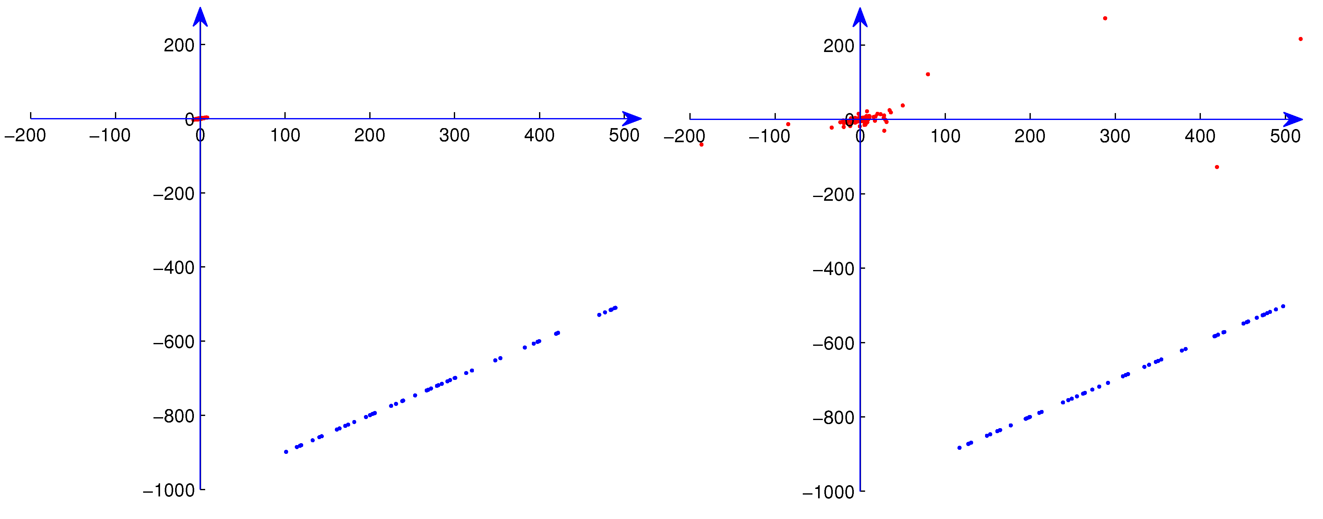
. We also generated data sets consisting of data from the distributions described above along with
,
and
patterned artificial outliers that represent clutter. For the one-distribution situation, artificial outliers were set up using a uniform statistical distribution on the
diamond with radius 1000 in the
-direction window
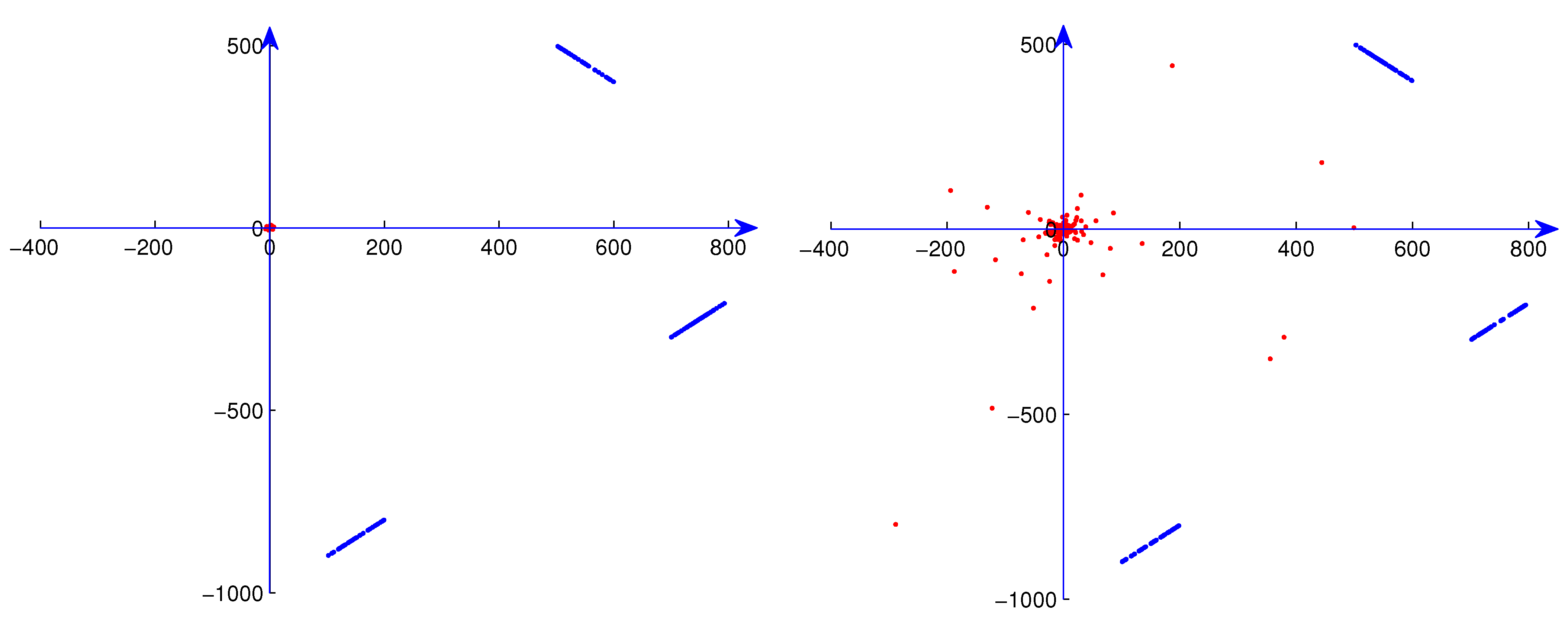
. For the three-superimposed-distribution situation, artificial outliers were set up using uniform statistical distributions on the
diamond with radius 1000 in the three different
-direction windows
,
and
. In Figs. 5, 6, 7 and 8, we present examples of 500-point data sets with 10% artificial outliers (depicted by blue dots) for one Gaussian distribution, one Student
t distribution, three superimposed Gaussian distributions and three superimposed Student
t distributions (points from distributions depicted by red dots), respectively.
Figure 3.
Sample from one Gaussian distribution with 10% artificial outliers.
Figure 3.
Sample from one Gaussian distribution with 10% artificial outliers.
Figure 4.
Sample from three superimposed Gaussian distributions with 10% artificial outliers.
Figure 4.
Sample from three superimposed Gaussian distributions with 10% artificial outliers.
For each type of data, we carried out 100 computational experiments, each time with a new sample from the statistical distribution(s), including the uniform distributions that generated the outliers. To measure the accuracy of the results, we calculated the average and standard deviation (over 100 computational experiments) of the error of each main
direction and the average and standard deviation of the error of the median radius in that direction vs. the theoretical values of the direction of maximum spread and the median radius in that direction of the continuum distribution. In
Table 1,
Table 2,
Table 3,
Table 4 and
Table 5, we present computational results for the sets of 500 points. Computational results for 50 and 150 points were analogous to those for 500 points.
Table 1.
Average error (av. error) and standard deviation of the error (std. dev.) of direction θ for one Gaussian distribution.
Table 1.
Average error (av. error) and standard deviation of the error (std. dev.) of direction θ for one Gaussian distribution.
| | Standard PCA | Croux+Ruiz-Gazen | Ke+Kanade | MCDA |
|---|
| av. error | 0.00005 | | | |
| std. dev. | 0.0051 | 0.0563 | 0.0084 | 0.0105 |
| av. error | | 0.0219 | — | 0.0349 |
| std. dev. | 0.0901 | 0.1733 | — | 0.1683 |
Table 2.
Average error (av. error) and standard deviation of the error (std. dev.) of direction θ for one Gaussian distribution with 10% artificial outliers.
Table 2.
Average error (av. error) and standard deviation of the error (std. dev.) of direction θ for one Gaussian distribution with 10% artificial outliers.
| | Standard PCA | Croux+Ruiz-Gazen | Ke+Kanade | MCDA |
|---|
| av. error | 1.0046 | | 0.9148 | |
| std. dev. | 0.0184 | 0.0837 | 0.0243 | 0.0114 |
| av. error | 261.9384 | 0.3185 | — | 0.1138 |
| std. dev. | 3.4384 | 0.1482 | — | 0.2028 |
Table 3.
Average error (av. error) and standard deviation of the error (std. dev.) of direction θ for one Student t distribution.
Table 3.
Average error (av. error) and standard deviation of the error (std. dev.) of direction θ for one Student t distribution.
| | Standard PCA | Croux+Ruiz-Gazen | Ke+Kanade | MCDA |
|---|
| av. error | 0.0353 | 0.0614 | 0.0474 | 0.0163 |
| std. dev. | 0.1983 | 0.0743 | 0.1738 | 0.01717 |
| av. error | 147.2380 | | — | 0.1438 |
| std. dev. | 258.1932 | 0.1692 | — | 0.2302 |
Table 4.
Average error (av. error) and standard deviation of the error (std. dev.) of direction θ for one Student t distribution with 10% artificial outliers.
Table 4.
Average error (av. error) and standard deviation of the error (std. dev.) of direction θ for one Student t distribution with 10% artificial outliers.
| | Standard PCA | Croux+Ruiz-Gazen | Ke+Kanade | MCDA |
|---|
| av. error | 1.0023 | 0.0624 | | |
| std. dev. | 0.2683 | 0.1744 | 0.2038 | 0.0234 |
| av. error | 385.4844 | | — | 0.2301 |
| std. dev. | 212.3327 | 0.2732 | — | 0.2289 |
Table 5.
Average error (av. error) and standard deviation of the error (std. dev.) of direction θ calculated by MCDA for three superimposed distributions without and with 10% artificial outliers.
Table 5.
Average error (av. error) and standard deviation of the error (std. dev.) of direction θ calculated by MCDA for three superimposed distributions without and with 10% artificial outliers.
| Distribution | av. error | std. dev. |
|---|
| | | 0.0103 |
| 3 Gaussians | 0.0124 | 0.0201 |
| | 0.0111 | 0.0103 |
| | | 0.0221 |
| 3 Gaussians with outliers | | 0.0252 |
| | 0.0124 | 0.0110 |
| | | 0.0224 |
| 3 Student t | 0.0130 | 0.0202 |
| | | 0.0193 |
| | 0.0143 | 0.0224 |
| 3 Student t with outliers | | 0.0252 |
| | 0.0130 | 0.0243 |
| | 0.0832 | 0.1593 |
| 3 Gaussians | 0.1291 | 0.1788 |
| | 0.1402 | 0.1891 |
| | 0.1382 | 0.1632 |
| 3 Gaussians with outliers | 0.1389 | 0.1738 |
| | 0.1537 | 0.1838 |
| | 0.1839 | 0.2582 |
| 3 Student t | 0.1783 | 0.2633 |
| | 0.1478 | 0.2537 |
| | 0.1987 | 0.2638 |
| 3 Student t with outliers | 0.1733 | 0.2837 |
| | 0.2018 | 0.2738 |
Remark 4 Since MCDA is an method, one may ask why the accuracy of the results is measured using averages and standard deviations rather than, for example, measures such as medians and other quantiles. The statistical distributions of the directions and median radii that are calculated by MCDA are zero-tailed and (apparently) light-tailed, respectively, which indicates that averages and standard deviations are more appropriate measures than quantiles.
Remark 5 No results for Ke and Kanade’s method are provided in
Table 1,
Table 2,
Table 3 and
Table 4 because Ke and Kanade’s method does not yield radius information.
The results in
Table 1 indicate that, as theoretically predicted, standard PCA performs better than any of the other three methods for data from one single Gaussian distribution. The results in
Table 2,
Table 3 and
Table 4 indicate that, as expected, standard PCA does not handle data with artificial outliers and/or from heavy-tailed distributions well. The results in
Table 2,
Table 3 and
Table 4 show, consistent with theoretical and computational evidence available in the previous literature, the advantages of Croux and Ruiz-Gazen’s projection-pursuit method and of Ke and Kanade’s
factorization method over standard PCA. These results also show in nearly all cases a marked advantage of
MCDA over Croux and Ruiz-Gazen’s projection-pursuit and Ke and Kanade’s
factorization. For the multiple superimposed distributions considered in
Table 5, standard PCA, Croux and Ruiz-Gazen’s projection-pursuit and Ke and Kanade’s
factorization each provide only one main direction for the superimposed distributions and do not yield any meaningful information about the individual main directions. For this reason, no results for these three methods are presented in
Table 5. It is worth noting in
Table 5 that the accuracy of
MCDA for three superimposed distributions without and with artificial outliers is just as good as the accuracy of
MCDA for single distributions without and with artificial outliers.
As the computing times reported in
Table 6 indicate, 2D
MCDA in its current implementation costs 30 to 40 times as much as standard PCA, roughly 3 times as much as Ke and Kanade’s factorization and 30% to 40% less than Croux and Ruiz-Gazen’s projection-pursuit (all methods sequentially implemented). The wide applicability of
MCDA in comparison with Ke and Kanade’s factorization method justifies an increase of computing time by a factor of 3. Moreover, the computing time of
MCDA is likely to decrease as the method is further investigated and more efficient implementations are designed.
Table 6.
Sequential computing times for generating the results in Table 1, Table 2, Table 3, Table 4 and Table 5 by the four methods.
| Data of | Standard PCA | Croux+Ruiz-Gazen | Ke+Kanade | MCDA |
|---|
| Table 1 | 3.398ms | 177.832ms | 32.921ms | 107.382ms |
| Table 2 | 4.411ms | 198.833ms | 33.477ms | 116.504ms |
| Table 3 | 3.667ms | 197.221ms | 48.133ms | 131.338ms |
| Table 4 | 5.277ms | 210.442ms | 55.672ms | 147.185ms |
| | | | | 225.348ms |
| Table 5 | | | | 248.392ms |
| | | | | 299.392ms |
| | | | | 335.429ms |
Computational results for 5% artificial outliers were analogous to the results for 10% artificial outliers. Computational results for MCDA with 20% artificial outliers in the data were not as accurate as those for 10% outliers. A quantitative description of the robustness of MCDA in terms of breakdown point (proportion of outliers beyond which the method produces errors that are arbitrarily large) or influence function (how the result changes when one point is changed) will depend not only on the radii and angular coordinates of the points that are changed but also on clustering patterns of these points in relation to the other points. This task is beyond the scope of this paper but will be an objective of future research.
The results in
Table 1,
Table 2,
Table 3,
Table 4 and
Table 5 indicate that, for the data considered here,
MCDA always outperforms standard PCA in accuracy except when the data come from one single Gaussian distribution and that
MCDA outperforms two robust PCAs in accuracy in nearly all cases in accuracy in nearly all the cases presented here. These computational results are consistent with the theoretically known fact that standard PCA is optimal for one single Gaussian distribution. Interestingly, however, the results in
Table 1 indicate that
MCDA performs quite well—albeit sub-optimally—for one single Gaussian distribution. Thus, there is no major disadvantage in using
MCDA as a default PCA (instead of standard PCA), since it performs well both for the cases when standard PCA is known to be optimal and, as we have seen, for the many other cases when standard PCA and robust PCAs perform less well, poorly or not at all.
5. Conclusions and Future Work
The assumptions underlying
MCDA are less restrictive and more practical than those underlying standard PCA and currently available robust PCAs. The 2D
MCDA that we have developed differs from standard PCA and all previously proposed robust PCAs in that it (1) allows use of a wide variety of distance functions in the data space (while noting the advantages of using the
norm to define the distance function); (2) replaces all (not just some) of the
-based procedures and concepts in standard PCA with
-based procedures and concepts; (3) has a theoretical foundation in heavy-tailed statistics but works well for data from both heavy-tailed and light-tailed distributions; (4) is applicable for data that need not have (but can have) mutually orthogonal main directions, can have multiple spokes and can contain patterned artificial outliers (clutter) and (5) does not require assumption of sparsity of the principal components or of the error. Most of the robust PCAs (with the exception of Ke and Kanade’s) that have previously been proposed in the literature involve use of the
norm not at all or only to a limited extent and continue to rely on
-based items including singular values, inner products, orthogonal projection, averaging and second moments (variances, covariances). The
MCDA that we propose comes exclusively from a unified theoretical framework based on the
norm. The computational results presented in
Section 4 show that the
MCDA proposed here significantly outperforms not only the standard PCA but also two robust PCAs in terms of accuracy.
This
MCDA is a foundation for a new, robust procedure that can be used for identification of dimensionality, identification of structure (including nonconventional spoke structure) and data compression in
,
, a topic on which the authors of this paper are currently working. In designing
MCDA for higher dimensions, the guiding principles will continue to be direct connection with heavy-tailed statistics and exclusive reliance on
operations. The higher-dimensional versions of Steps 1 and 2 of
MCDA are feasible as long as appropriate higher-dimensional angular coordinates can be defined. The reader may question whether the “
polar coordinates” that are used in 2D can be extended to
n dimensions. Indeed they can in the following manner. In direct analogy to the definition of the polar coordinate
in (
8) in two dimensions, one defines angular coordinates one defines
angular coordinates of an
n-dimensional data point
to be the quotients with the components of the point as numerators and the
radius
of the point as denominators. In passing we note that these higher-dimensional
angular coordinates are computationally cheaper than standard
hyperspherical angular coordinates, which require calculation of square roots of sums of squares.
For samples of M vectors in , , the cost of classical PCA is . The costs of Croux and Ruiz-Gazen’s method and of Ke and Kanade’s method are not specified in the literature but apparently scale linearly with respect to sample size M. We hypothesize that the extension of MCDA to higher dimensions will have a sequential cost of and will be comparable with or lower than the cost of competing robust PCAs.
MCDA is expected to be a robust tool in terrain modeling, geometric modeling, image analysis, information mining, face/object recognition and general pattern recognition. As suggested by the computational results presented in the present paper, it is expected that MCDA will be particularly useful for pattern recognition under patterned clutter. For example, MCDA will be useful for identification of objects behind occlusions because it handles the occlusions as outliers and does not require a separate step of segmenting out the occlusions. This capability will provide a basis for going directly from point cloud to robust semantic labeling.

