Minimization principles based on the l¹ and L¹ norms have recently rapidly become more common due to discovery of their important roles in sparse representation in signal and image processing [1,2], compressive sensing [3,4], shape-preserving geometric modeling [5,6] and robust principal component analysis [7,8,9]. In compressive sensing and sparse representation, it is known that, under proper sparsity conditions (for example, the restricted isometry property [3,4]), l¹ solutions are equivalent to “l⁰ solutions”, that is, the sparsest solutions, an important result because it allows one to find the solution of a combinatorially expensive l⁰ maximum-sparsity minimization problem by a polynomial-time linear programming procedure for minimizing l¹ functionals. When the data follow heavy-tailed statistical distributions and the tails of the distributions are “not too heavy,” various l¹ minimization principles, in the form of calculation of medians and quantiles, are primary choices that are efficient and robust against the many outliers [10,11,12]. Such distributions correspond to the uncertainty in many human-based phenomena and activities, including the Internet [13,14], finance [15,16] and other human and physical phenomena [16]. l¹ minimization principles are applicable also to data from light-tailed distributions such as the Gaussian, but, for such distributions, are less efficient than classical procedures (calculation of standard averages and variances).

When tails of the distributions are so heavy that even l¹ minimization principles do not exist, one needs to consider using l^p minimization principles with 0 < p < 1, a topic on which investigation has recently started [2,3,17,18,19,20]. l^p minimization principles, 0 < p < 1, are of interest because they produce solutions that are in general sparser, that is, closer to l⁰ solutions, than l¹ minimization principles [20]. However, when 0 < p < 1, solving l^p minimization principles is generically combinatorially expensive (NP-hard) [18], because l^p minimization principles can have arbitrarily large numbers of local minima. (“Generically” means “in the absence of additional information.”) Investigations about polynomial-time l^p minimization, 0 < p < 1, have focused on (1) obtaining local rather than global solutions [2,18,20] and (2) achieving a global minimum by restricting the class of problems to those with sufficient sparsity [3,17,19] (the approach used in compressive sensing). However, local solutions often differ strongly from global solutions and sparsity restrictions are often not applicable. The fact that the l⁰ solution is, relative to other potential solutions, the sparsest solution does not imply that this solution is sparse to any specific degree. The sparsest solution may not be sparse in any absolute sense at all; it is just sparser than any other solution.

The approach that we will investigate in the present paper shares with compressive sensing the strategy of restricting the nature of the problem to achieve polynomial-time performance. However, we do so not by requiring sparsity to some a priori set level but rather by restricting the data to come from a wide class of statistical distributions, an approach not previously considered in the literature. This restriction turns out to be mild, often verifiable and often realistic since the problem as posed is often meaningful only when the data come from a statistical distribution. The approach in this paper differs from the approaches in the previous literature on l^p minimization principles also in a second way, namely, in that it starts the investigation of l^p minimization principles from consideration of their continuum analogues, L^p minimization principles.

The classes of L^p and l^p minimization principles that we will investigate in this paper are those that represent univariate continuum L^p averaging and discrete l^p averaging, defined as follows. Univariate L^p and l^p averages are the real numbers a at which the following functionals A and B achieve their respective global minima: (1) where ψ is a probability density function (pdf) that satisfies the conditions given below, and (2) where the x_i are data points from the distribution with pdf ψ. The pdf ψ is assumed to have measurable second derivative and to satisfy the following two conditions:

radially strictly monotonically decreasing outwards from the mode (3a)

Without loss of generality, we assume that the mode, that is, the x at which ψ achieves its maximum, is at the origin.

In a departure from the traditional use of x as the independent variable of a univariate pdf, we will express univariate pdfs in radial form with r being the radius measured outward from the mode of the distribution. (This notation is chosen to allow natural generalization to higher dimensions in the future.) With the notation g(r) = ψ(–r) and f(r) = ψ(r), r ≥ 0, functional A can be rewritten in the form (4) Since functional (4) is finite only when (5) the mean (L² average) does not exist for distributions with β ≤ 3 and even the median (L¹ average) does not exist for distributions with β ≤ 2. For example, the median does not exist for the Student t distribution with one degree of freedom because β = 2 for this distribution. To create meaningful “averages” in these cases, weighted and trimmed sample means have been proposed with success [21]. However, weighted and trimmed sample means require a priori knowledge of the specific distribution and/or of various parameters, knowledge that is often not available. Minimization of the L^p functional (4) or of the l^p functional (2) is, when 0 < p < min{1, β−1}, an alternative for creating an “average” for a heavy-tailed distribution or of a sample thereof.

In the present paper, we will investigate whether, by providing only the information that the data come from a “standard” statistical distribution that satisfies Conditions (3), the L^p and l^p averaging functionals A and B can be minimized in a way that leads to polynomial-time minimization of general L^p and l^p functionals. Specifically, in the next two sections, we will investigate to what extent the L^p and l^p averaging functionals are devoid of local minima other than the global minimum, a key feature in this process. For illustration of the theoretical results, we will present computational results for the following three types of distributions:

Distribution 1: Gaussian (light-tailed distribution) distribution with probability density function (6)

Distribution 2: Symmetric heavy-tailed distribution with probability density function (7a) (7b) where (7c) (For Distribution 2, the β of condition (3b) is α.)

Distribution 3: Asymmetric heavy-tailed distribution with probability density function (8a) (8b) (right tail heavier than left tail), where (8c) (For Distribution 3, the β of condition (3b) is (1 + α)/2.)

In Distributions 2 and 3, α is a real number > 1. Gaussian Distribution 1 is used to show that the results discussed here are applicable not only to heavy-tailed distributions but also to light-tailed distributions. These results are applicable a fortiori to compact distributions with no tails at all (tails uniformly 0). (Analysis and computations were carried out with the uniform distribution and with a pyramidal distribution, two distributions with no tails, but these results will not be discussed here.) While L^p and l^p averages can be calculated for light-tailed and no-tailed distributions, there are more meaningful and more efficient ways, for example, arithmetic averaging, to calculate central points of light-tailed and no-tailed distributions. L^p and l^p averages are most meaningful for heavy-tailed distributions.

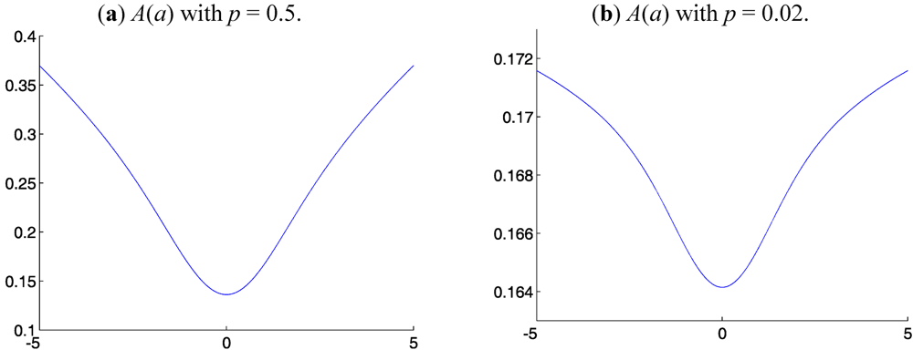
We present in Figure 1, Figure 2 and Figure 3 the functionals A(a) for Distributions 1-3, respectively, for various p. These functionals A(a) have one global minimum at or near r = 0, no additional minima, are convex in a neighborhood of the global minimum and are concave outside of this neighborhood. The fact that the A(a) are not globally convex is not important. Each A(a) is radially monotonically increasing outward from its minimum, which is sufficient to guarantee that there is only one global minimum and that there are no other local minima. On every finite closed interval in Figure 1, Figure 2 and Figure 3 that does not include the global minimum, the derivative dA/da is bounded away from 0. Hence, in all these cases, standard line-search methods converge to the global minimum in polynomial time. The structure of A(a) seen in Figure 1, Figure 2 and Figure 3 is due to the fact that A(a) is based on a probability density function with strictly monotonically decreasing density in the radial directions outward from the mode. This structure does not generically occur for density functions f(r) and g(r) representing, for example, irregular scattered clusters. However, averaging in general and L^p averaging in particular make little sense when the data are clustered irregularly. The computational results presented in Figure 1, Figure 2 and Figure 3 suggest the hypothesis that, under “normal” statistical conditions on the data, L^p averaging is well posed and computationally tractable. In the remainder of this section, we will investigate portions of this hypothesis.

The structure of the L^p averaging functional A(a) seen in Figure 1, Figure 2 and Figure 3 and described in the previous paragraph occurs for all symmetric distributions, a situation that can be shown as follows. For symmetric distributions (that is, those for which g(r) = f(r)), the L^p averaging functional A(a) can be written as (9) A(a) is symmetric around a = 0, so we need consider only the behavior of A(a) for a ≥ 0. For a ≥ 0, (10) and (11)

One computes expressions (10) and (11) by differentiating the right sides of expressions (9) and (10), respectively, with respect to a. One expresses the integral to be differentiated as the sum of an integral on (0,a) and an integral on (a,∞) and differentiates these two integrals separately. To simplify dA/da to the form given in (10), one integrates by parts and combines the two resulting integrals. From these expressions, one obtains first that dA/da(0) = 0 and d²A/da²(0) > 0, that is, there is a local minimum at a = 0 and second that, for all a > 0, dA/da(a) > 0, that is, A is strictly monotonically increasing for a > 0. Thus, for symmetric pdfs, A(a) has its global minimum at a = 0, that is, the L^p average exists and is equal to the mode of the distribution. There are no places where dA/da = 0 other than at a = 0 and, on every finite closed interval that does not include the mode 0, dA/da is bounded away from 0. Standard line-search methods for calculating the minimum of this A(a) are thus globally convergent.

A general analytical structure for asymmetric distributions analogous to that described above for symmetric distributions is not yet available because, for asymmetric distributions, the properties of A(a) depend on additional properties of the probability density functions f(r) and g(r) that have not yet been clarified. Most of the previous statistical research about two-tailed distributions that extend infinitely in each direction has been focused on symmetric distributions and it is the symmetric case on which we will focus in the remainder of this paper.

It is meaningful to calculate an l^p average of a discrete set of data, that is, the point at which B(a) achieves its global minimum, only for data from a distribution that satisfies Conditions (3) and for which the L^p average exists, that is, for which 0 < p < β − 1. We propose the following algorithm.

Algorithm 1: Algorithm for l^p Averaging

STEP 1. Sort the data x_i, i = 1, 2, . . . , I, from smallest to largest. (To avoid proliferation of notation, use the same notation x_i, i = 1, 2, . . . , I, for the data after sorting as before.)

STEP 2. Choose an integer q that represents the number of neighbors of a given point in the sorted data set in each direction (lower and higher index) that will be included in a local set of indices to be used in the “window” in Step 4. (The “window size” is thus 2q + 1)

STEP 3. Choose a point x_j from which to start. (The median of the data, that is, the l¹ average, is generally a good choice for the initial x_j.)

STEP 4. For each k, j − q ≤ k ≤ j + q, calculate B(x_k).

STEP 5. If the x_k that yields the minimum of the B(x_k) calculated in Step 4 is x_j, stop. In this case, x_j is the computed l^p average of the data. Otherwise, let x_k be a new x_j and return to Step 4.

STEP 6. If convergence has not occurred within a predetermined number of iterations, stop and return an error message.

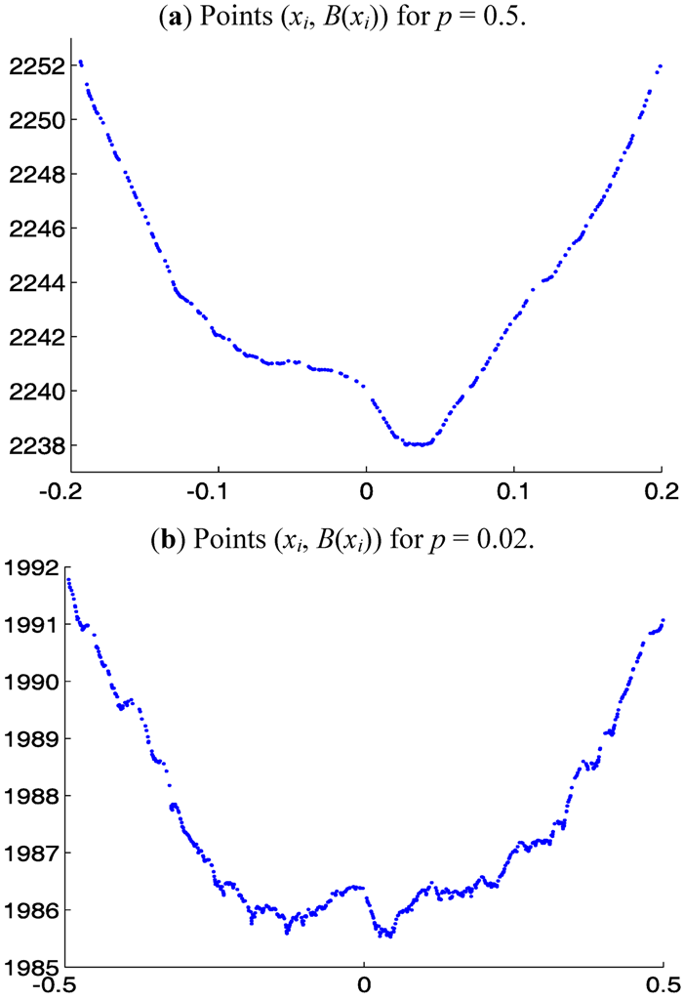
Remark 1. Algorithm 1 considers the values of B(a) only at the data points x_i and not between data points. For a strictly between two consecutive data points x_i and x_i+1, B(a) is concave and is above the line connecting (x_i,B(x_i)) and (x_i+1,B(x_i+1)), so a minimum cannot occur there. It is sufficient, therefore, to consider only the values of B at the points x_i when searching for a minimum. A graph of the points (x_i,B(x_i)), i = 1, 2, . . . , I, approximates the graph of the continuum L^p functional A(a), which, for symmetric distributions, has only one local minimum, namely, its global minimum. The graph of the points (x_i,B(x_i)) may have some relatively shallow local minima produced by the irregular spacing of the x_i (cf. Figure 4 below) and/or the asymmetry of the distribution. The window structure of Algorithm 1 is designed to allow the algorithm to “jump over” these local minima on its way to the global minimum.

Remark 2. The cost of Algorithm 1 is polynomial, namely, the cost O(I log I) of the sorting operation of Step 1 plus the cost of the iterations of Step 4, namely, O(I²) (= the number of iterations, which cannot exceed O(I), times the cost O(I) of calculating each iteration). Analogous algorithms for higher-dimensional averages are expected to retain this polynomial-time nature.

In computational experiments, we used samples of size I = 2000 from the symmetric heavy-tailed Distribution 2 with various α, 1 < α ≤ 3, and window sizes 2q + 1 = 7, 9, 11, . . . , 25. For comparison with Figure 2, we present in Figure 4 the graphs of the points (x_i, B(x_i)) for the sample from Distribution 2 with α = 2 and p = 0.5 and 0.02. The starting point for Step 3 of the Algorithm 1 was chosen to be x_I−2q, a point near the end of the right tail (beyond the limited domains shown in Figure 4). As mentioned in Step 3 of Algorithm 1, the median of the data is a much better choice for a starting point. However, choosing a point near the right tail makes the iterations of Algorithm 1 traverse a large distance before converging to an approximation of the l^p average and thus provides an excellent test for the robustness of Algorithm 1. Computational results for p = 0.5, 0.1 and 0.02 and for window sizes 2q + 1 = 7, 13, 19 and 25 are presented in Table 1, Table 2, Table 3 and Table 4. For reference, we note that the continuum L^p averages of Distribution 2, when they exist, that is, when p < α − 1, are all 0. Thus, the errors of the l^p averages in Table 1, Table 2, Table 3 and Table 4 are the same as the l^p averages themselves.

The entries in Table 1, Table 2, Table 3 and Table 4 indicate that, for all cases with p < α − 1, the l^p average computed by Algorithm 1 is an excellent approximant of the L^p average 0 given the large number of outliers and the huge spread of the data in Distribution 2. (For α = 3 and α = 1.02, the ranges of the data are [−16.0, 22.6] and [−6.44 × 10¹⁵⁴, 5.02 × 10¹⁶⁹], respectively. For α = 2, 1, 1.5, 1.1, 1.05, 1.04 and 1.03, the ranges are between these two ranges.) The entries for p = 0.5 with α = 1.5 and for p = 0.1 with α = 1.1, 1.05, 1.04 and 1.03 in Table 1 and Table 2 indicate that, in a few cases when p is equal to or only slightly greater than α − 1, the l^p average yielded by Algorithm 1 can still be a good approximant of the center of the distribution in spite of the fact that the l^p average is theoretically meaningful only when p < α − 1. The entries for p = 0.5 with α = 1.1, 1.05, 1.04, 1.03 and 1.02 and for p = 0.1 with α = 1.02 indicate that, in accordance with expectations, when p is significantly greater than α − 1, the l^p average produced by Algorithm 1 is not a meaningful approximant of the center of the distribution. Since larger window size is of assistance when attempting to “jump over” local minima, it is expected that l^p averages should converge to the L^p average 0 as the window size 2q + 1 increases (and as the sample size increases). The results in Table 1, Table 2, Table 3 and Table 4 confirm that, for the samples used in these calculations, increasing the window size does indeed increase the accuracy of the l^p averages as approximations of the L^p average 0. In addition, the results in Table 3 and Table 4 for p < α − 1 show that, for the samples used in these calculations, there is an optimal q, namely, q = 19 that produces l^p averages that are just as good as the l^p averages produced by the larger q = 25 but (due to smaller window size) requires less computational effort.

Algorithm 1 is applicable to heavy-tailed distributions in general but the rule for choosing q will certainly be dependent on the specific class of distributions under consideration. While this rule is not yet known precisely, we can provide here a description of the principles that will likely be the foundations for the rule. The choice of q is related to how wide the local minima in the discrete functional B are. The local minima of B occur at places where there are clusters of data points (due to expected statistical variation in the sample). Understanding the relationships between (1) the clustering properties of samples from the given class of distributions, (2) the widths of the local minima as functions of the clustering and (3) the p-dependent analytical properties of functional B will likely yield the rule for choosing q.

The wide-spread impression that minimization of L^p and l^p functionals, 0 < p < 1, is combinatorially expensive is valid for general situations in which no structure of the data is known. However, the results in this paper suggest that, when the data come from an appropriate statistical distribution, L^p and l^p averages can be calculated in polynomial time. The approach of the paper is applicable without precise knowledge of the parameters of the distribution. One does not need precise knowledge of the parameters but rather only generalizations of Conditions (3), an upper bound on the exponent −β of the tail density and additional conditions for asymmetric distributions and for setting up a rule for choosing q in Algorithm 1.

Topics for future research include

Quantitative rules for using information about the underlying continuum distribution to choose the q of Algorithm 1 based on a user’s preferred tradeoff between maximum accuracy and minimum computational burden

Many phenomena in human-based areas (sociology, cognitive science, psychology, economics, human networks, social media, etc.) are increasingly known to be represented by data that have large numbers of outliers and belong to very heavy-tailed distributions, which suggests that L^p and l^p averaging, L^p and l^p regression and more general L^p and l^p minimization tasks, 0 < p < 1, will be important in practice. The results of the present paper provide the first indication that one may be able to solve, in polynomial time, generically combinatorially expensive L^p and l^p minimization problems for these phenomena by requiring only “natural” statistical structure without having to impose restrictions such as sparsity and without having to accept suboptimal local solutions instead of optimal global solutions.