A Catalog of Self-Affine Hierarchical Entropy Functions

Abstract
: For fixed k ≥ 2 and fixed data alphabet of cardinality m, the hierarchical type class of a data string of length n = kj for some j ≥ 1 is formed by permuting the string in all possible ways under permutations arising from the isomorphisms of the unique finite rooted tree of depth j which has n leaves and k children for each non-leaf vertex. Suppose the data strings in a hierarchical type class are losslessly encoded via binary codewords of minimal length. A hierarchical entropy function is a function on the set of m-dimensional probability distributions which describes the asymptotic compression rate performance of this lossless encoding scheme as the data length n is allowed to grow without bound. We determine infinitely many hierarchical entropy functions which are each self-affine. For each such function, an explicit iterated function system is found such that the graph of the function is the attractor of the system.1. Introduction
A traditional type class consists of all permutations of a fixed finite-length data string. There is a well-developed data compression theory in which strings in a traditional type class are losslessly encoded into fixed-length binary codewords [1]. One can generalize the notion of traditional type class and the resulting data compression theory in the following natural way Let T be a finite rooted tree; an isomorphism of T is a one-to-one mapping of the set of vertices of T onto itself which preserves the parent-child relation. Let n be the number of leaves of T, let (T) be the set of leaves of T, and let σ be a one-to-one mapping of {1, 2, …, n} onto (T). Suppose (X1, X2, …, Xn) is a data string of length n. Define the T-type class of (X1, …, Xn) to consist of all strings (Y1, Y2, …, Yn) for which there exists an isomorphism ϕ of T such that
Consider the depth one tree T = T1(n) in which there are n children of the root, which are the leaves of the tree. Then, the notion of T1(n)-type class coincides with the notion of traditional type class. Now let n = kj for positive integer j and integer k ≥ 2. Consider the depth j tree T = Tj(k) with n leaves such that each non-leaf vertex has k children. Then, a Tj(k)-type class is called a hierarchical type class, and k is called the partitioning parameter of the class. In the paper [2], we dealt with hierarchical type classes in which the partitioning parameter is k = 2. In the present paper, we deal with hierarchical type classes in which the partitioning parameter is an arbitrary k ≥ 2.
Given a hierarchical type class S, there is a simple lossless coding algorithm which encodes each string in S into a fixed-length binary codeword of minimal length, and decodes the string from its codeword. This algorithm is particularly simple for the case when the partitioning parameter is k = 2, and we illustrate this case in Example 1 which follows; the case of general k ≥ 2 is discussed in [3]. In Example 1 and subsequently, x1 * x2 * … * xk shall denote the data string obtained by concatenating together the finite-length data strings x1, x2, …, xk (left to right).
Example 1
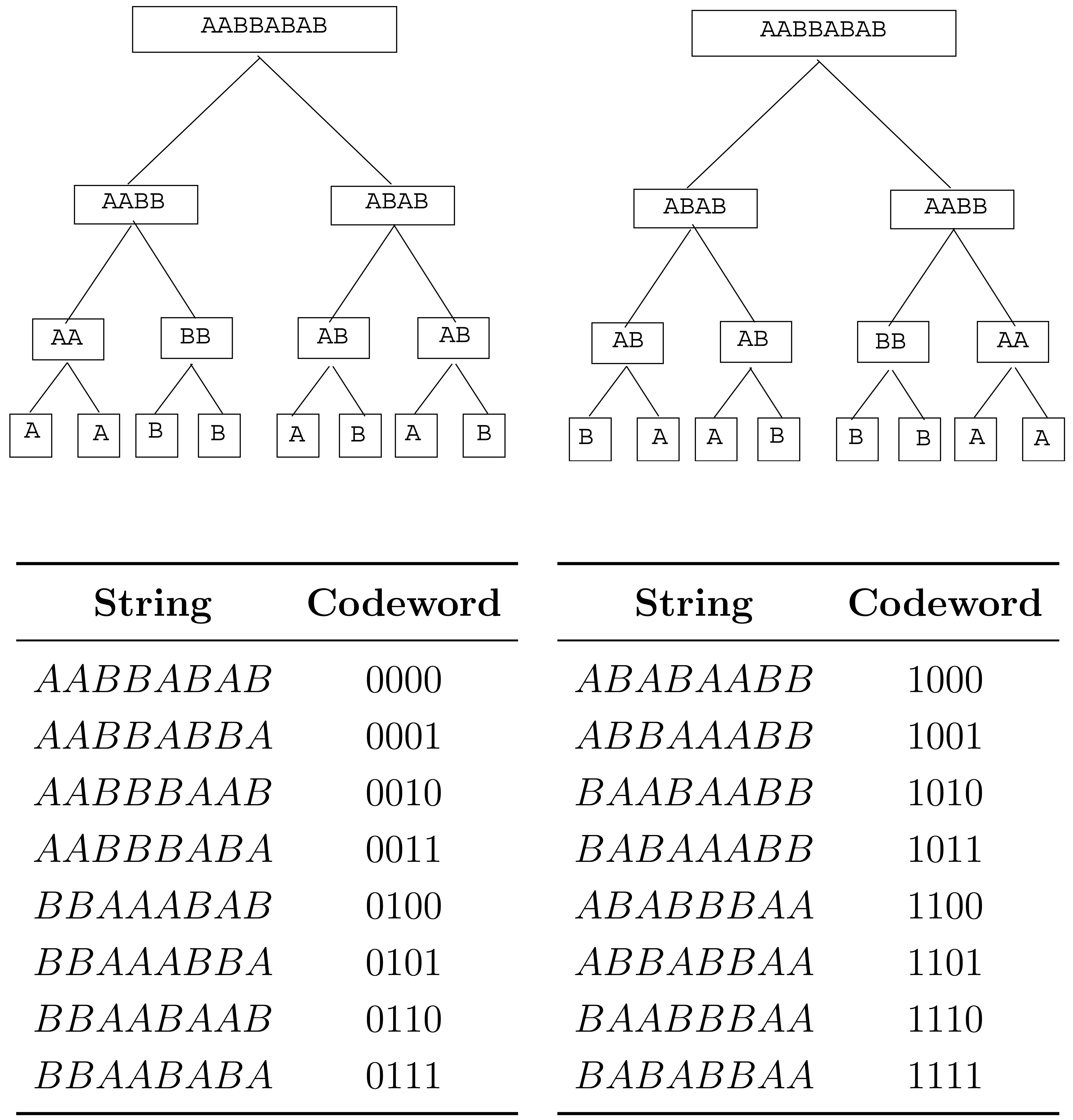
Let k = 2, and let S be the hierarchical type class of data string AABBABAB. The 16 strings in S are illustrated in Figure 1. Each string x ∈ S has a tree representation in which each vertex of tree T3(2) is assigned a label which is a substring of x. This assignment takes place as follows.
The leaves of the tree, traversed left to right, are labeled with the respective left-to-right entries of the data string x.
For each non-leaf vertex v, if the strings labeling the left and right children of v are xL, xR, respectively, then the string labeling v is xL * xR if xL precedes or is equal to xR in the lexicographical order, and is xR * xL, otherwise.
In Figure 1, we have illustrated the tree representations of the strings AABBABAB and BAABBBAA. The root label of all 16 tree representations will be the same string, namely, the first string in S in lexicographical order, which is the string AABBABAB in this case. Each string in S is encoded by visiting, in depth-first order, the non-leaf vertices of its tree representation whose children have different labels. Each such vertex is assigned bit 0 if its label is xL * xR, where xL, xR are the labels of its left and right children, and is assigned bit 1 otherwise (meaning that the label is xR * xL). The resulting sequence of bits, in the order they are obtained, is the codeword of the string. Since both encoder and decoder will know what hierarchical type class is being encoded, the decoder will know what the root label of the tree representation should be, and then the successive bits of the codeword allow the decoder to grow the tree representation from the root downward.
Before discussing the nature of the results to be obtained in this paper, we need some definitions and notation. Fix integers m, k ≥ 2, which serve as parameters in the subsequent development; k is the partitioning parameter already introduced, and m is called the “alphabet cardinality parameter” because we shall be dealing with an m-letter data alphabet, denoted
 m = {a1, a2, …, am}. For each j ≥ 0, we define a j-string x to be a string of length kj over
m. Note that if j ≥ 1, for each j-string x there is a unique k-tuple (x1, x2, …, xk) whose entries are (j − 1)-strings such that x = x1*x2*…*xk; this k-tuple is called the k-partitioning of x. If S1, S2, …, Sk are non-empty sets of j-strings, let S1 * S2 * … * Sk be the set of all (j + 1)-strings of the form x1 * x2 * … * xk, where xi belongs to Si for i = 1, 2, …, k. The 0-strings are the individual letters in
m.
m = {a1, a2, …, am}. For each j ≥ 0, we define a j-string x to be a string of length kj over
m. Note that if j ≥ 1, for each j-string x there is a unique k-tuple (x1, x2, …, xk) whose entries are (j − 1)-strings such that x = x1*x2*…*xk; this k-tuple is called the k-partitioning of x. If S1, S2, …, Sk are non-empty sets of j-strings, let S1 * S2 * … * Sk be the set of all (j + 1)-strings of the form x1 * x2 * … * xk, where xi belongs to Si for i = 1, 2, …, k. The 0-strings are the individual letters in
m.
We wish to formally define the family
 m,k of all hierarchical type classes in which the alphabet cardinality parameter is m and the partitioning parameter is k. Instead of using the tree isomorphism definition of hierarchical type class given at the beginning of the paper, we will use an equivalent inductive definition, which is more convenient in the subsequent development. First, we define the hierarchical type class of a 0-string to be the set consisting of the string itself. Given j-string x with j ≥ 1, and assume hierarchical type classes of (j − 1)-strings have been defined. Let (x1, …, xk) be the k-partitioning of x and let Si be the hierarchical type class of xi (i = 1, …, k). The hierarchical type class of x is then defined as
m,k is then the set of all hierarchical type classes, of all orders.We define the type of j-string x to be the vector (n1, …, nm) whose i-th component ni is the frequency of letter ai in x. For each j ≥ 0, let Λj (m, k) be the set of all types of j-strings. Let Λ(m, k) be the union of the Λj(m, k)'s for j ≥ 0, and let Λ+(m, k) be the union of the Λj(m, k)'s for j ≥ 1. A type in Λj(m, k) will be said to be of order j. If λ ∈ Λ(m, k), let ‖λ‖ denote the sum of the components of λ. If λ is of order j, then ‖λ‖ = kj. All strings in a hierarchical type class have the same type, because permuting a string does not change the type. This property is listed below, along with some other properties whose simple proofs are omitted.
Prop. 1: All strings in a hierarchical type class have the same type.
Prop. 2: For each j ≥ 0, the distinct hierarchical type classes of order j form a partition of the set of all j-strings.
Prop. 3: Let λ ∈ Λ(m, k), and let
![Algorithms 04 00307i3]() m,k(λ) denote the set of all hierarchical type classes in
m,k(λ) denote the set of all hierarchical type classes in
![Algorithms 04 00307i3]() m,k whose strings are of type λ. Then
m,k whose strings are of type λ. Then
![Algorithms 04 00307i3]() m,k(λ) forms a partition of the set of all strings of type λ.
m,k(λ) forms a partition of the set of all strings of type λ.Prop. 4: Let S ∈
![Algorithms 04 00307i3]() m,k be a hierarchical type class of order j ≥ 1. Then there is a k-tuple (S1, S2, …, Sk), unique up to permutation, such that each Si is a hierarchical type class of order j − 1 and S is expressible as Expression (1).
m,k be a hierarchical type class of order j ≥ 1. Then there is a k-tuple (S1, S2, …, Sk), unique up to permutation, such that each Si is a hierarchical type class of order j − 1 and S is expressible as Expression (1).
Global Hierarchical Entropy Function
The global hierarchical entropy function is the function H :
m,k → [0, ∞) such that
Lemma 1
Let S be a hierarchical type class of order j ≥ 1. Let (S1, S2, …, Sk) be the k-tuple of hierarchical type classes of order j − 1 associated with S according to Prop. 4, and let N(S) be the number of distinct permutations of this k-tuple. Then,
Proof
Represent S as the Expression (1). Formula (2) follows easily from this expression.
Remark
We see now how to inductively compute entropy values H(S), as follows. If S is of order 0, then |S| = 1 and so H(S) = 0. If S is of order j ≥ 1, assume all entropy values for hierarchical type classes of smaller order have been computed. Then Equation (2) is used to compute H(S).
Discussion
Let {Sj : j ≥ 1} be a sequence of hierarchical type classes from
m,k such that Sj is of order j (j ≥ 1). Consider the sequence of normalized entropies {H(Sj)/kj : j ≥ 1}. As j becomes large, the normalized entropy H(Sj)/kj approximates more and more closely the compression rate in bits per data sample that results from the compression scheme on Sj. It is therefore of interest to determine circumstances under which such a sequence of normalized entropies will have a limit that we can compute. We discuss our approach to this problem, which will be pursued in the rest of this paper. A hierarchical source is defined to be a family {S(λ) : λ ∈ Λ(m, k)} in which each S(λ) is a hierarchical type class selected from
m,k(λ). (We will also impose a natural consistency condition on how these selections are made in our formal hierarchical source definition to be given in the next section.) Let ℝ denote the real line, and let ℙm be the subset of ℝm consisting of all m-dimensional probability vectors. We consider ℙm to be a metric space with the Euclidean metric. For each λ ∈ Λ(m, k), let pλ be the probability vector λ/‖λ‖ in ℙm. Suppose there exists a (necessarily unique) continuous function h : ℙm → [0, ∞) such that for each p ∈ ℙm, and each sequence {λj : j ≥ 0} for which λj ∈ Λj(m, k) (j ≥ 0) and limj→∞ pλj = p, the limit property
2. Hierarchical Sources
This section is devoted to the discussion of hierarchical sources. The concept of hierarchical source was informally described in the Introduction. In Section 2.1., we make this concept formal. In Section 2.2., we define the entropy-stable hierarchical sources, which are the hierarchical sources that induce hierarchical entropy functions. In Section 2.3., we introduce a particular type of entropy-stable hierarchical source called finitary hierarchical source. The finitary hierarchical sources induce the hierarchical entropy functions that are the subject of this paper.
2.1. Formal Definition of Hierarchical Source
Let
= {S(λ) : λ ∈ Λ(m, k)} be a family of hierarchical type classes in which each class S(λ) belongs to the set of classes
m,k(λ). Then
is defined to be a (Λ(m, k)-indexed) hierarchical source if the following additional condition is satisfied.
Consistency Condition: For each S ∈
![Algorithms 04 00307i3]() of order > 0, each term in the k-tuple (S1, S2, …, Sk) associated with S in Prop. 4 also belongs to
of order > 0, each term in the k-tuple (S1, S2, …, Sk) associated with S in Prop. 4 also belongs to
![Algorithms 04 00307i3]() .
.
We discuss how the Consistency Condition gives us a way to describe every possible hierarchical source. Let Λ(m, k)k be the set of all k-tuples whose entries come from Λ(m, k). Let Φ(m, k) be the set of all mappings ϕ: Λ(m, k)+ → Λ(m, k)k such that whenever ϕ(λ) = (λ1, λ2, …, λk), we have
.
If λ is of order j, then each entry λi of ϕ(λ) is of order j − 1.
Each ϕ ∈ Φ(m, k) gives rise to a Λ(m, k)-indexed hierarchical source
ϕ = {Sϕ(λ) : λ ∈ Λ(m, k)}, defined inductively as follows.
If λ ∈ Λ(m, k) is of order 0, define class Sϕ(λ) to be the set {ai}, where ai is the unique letter in
![Algorithms 04 00307i2]() m whose type is λ.
m whose type is λ.If λ ∈ Λ(m, k)+, assume class Sϕ(λ*) has been defined for all types λ* of order less than the order of λ. Letting ϕ(λ) = (λ1, λ2, …, λk), define
From the Consistency Condition, all possible hierarchical sources arise in this way, that is, given any Λ(m, k)-indexed hierarchical source
, there exists ϕ ∈ Φ(m, k) such that
=
ϕ.
Another advantage of the Consistency Condition is that it allows the entropies of the classes in a hierarchical source to be recursively computed. To see this, let
= {S(λ) : λ ∈ Λ(m, k)} be a Λ(m, k)-indexed hierarchical source and choose ϕ ∈ Φ(m, k) such that
=
ϕ. Define Hϕ : Λ(m, k) → [0, ∞) to be the function which takes the value zero on Λ0(m, k), and for each λ ∈ Λ+(m, k),
2.2. Entropy-Stable Hierarchical Sources
The concept of entropy-stable source discussed in this section allows us to formally define the concept of hierarchical entropy function.
For each j ≥ 0, define the finite set of probability vectors
Let be the countably infinite set of probability vectors which is the union of the ℙm(j)'s.
Suppose we have a hierarchical source
= {S(λ) : λ ∈ Λ(m, k)}. For each j ≥ 0, let hj : ℙm(j) → [0, ∞) be the unique function for which
Suppose
Because of the increasing sets property Equation (4), p is a member of the set ℙm(j) for j sufficiently large. Consequently, hj(p) is defined for j sufficiently large, and so it makes sense to talk about the limit of the sequence {hj(p) : j ≥ 0}, if this limit exists. We define the source
to be entropy-stable if there exists a continuous function h : ℙm → [0, ∞) such that
. Henceforth, the terminology “hierarchical entropy function” denotes a function which is the hierarchical entropy function induced by some entropy-stable hierarchical source.2.3. Finitary Hierarchical Sources
If λ = (n1, n2, …, nm) is a type in Λ(m, k)+, define
Definitions
(m, k) is defined to be the set of all m-tuples whose entries come from {0, 1, …, k − 1} and sum to an integer multiple of k.
Ψ(m, k) is defined to be the set of all mappings ψ from (m, k) to the set of binary k × m matrices such that if r = (r1, …, rm) belongs to (m, k), then ψ(r) has left-to-right column sums r1, r2, …, rm and row sums all equal to (r1 + r2 + … + rm)/k. The set Ψ(m, k) is nonempty for each choice of parameters m, k ≥ 2 [4,5].
If ψ ∈ Ψ(m, k), define ψ* to be the unique mapping in Φ(m, k) which does the following. If λ = (n1, n2, …, nm) belongs to Λ(m, k)+, let A = ψ(r(λ)). Then ψ*(λ) = (λ1, λ2, …, λk), where
with A(i, 1 : m) denoting the i-th row of A.Suppose ψ ∈ Ψ(m, k) and let ϕ = ψ*. The Λ(m, k)-indexed hierarchical source {Sϕ : λ ∈ Λ(m, k)} defines a finitary source. For each choice of parameters m, k ≥ 2, since Ψ(m, k) is nonempty, there is at least one finitary Λ(m, k)-indexed hierarchical source. The word “finitary” is used to describe these sources because they are each definable in finite terms by the specification of mk|(m, k)| bits (the elements of a number of k × m binary matrices).
Example 2
Note that (1122) belongs to (4, 3). Suppose
Note that (7758) ∈ Λ+(4, 3), and that
Since ⌊(7758)/3⌋ = (2212), we see that ψ*(7758) = (λ1, λ2, λ3), where
Note that the splitting up of (7758) into the three types (3312), (2223), (2223) indeed does make sense because these latter three types sum to (7758) and are of order 2, one less than the order of (7758).
Example 3
Fix the alphabet cardinality parameter to be 2, and fix the partitioning parameter k to be any integer ≥ 2. Let (r1, r2) belong to (2, k). Then either (a) (r1, r2) = (0, 0) or (b) r1 + r2 = k. In case (a), we define ψ(r1, r2) to be the k × 2 zero matrix. In case (b), we define ψ(r1, r2) to be the k × 2 matrix whose first r1 rows are (1, 0) and whose last r2 rows are (0, 1). Letting ϕ = ψ*, we obtain finitary Λ(2, k)-indexed hierarchical source
ϕ.
Example 4
Now fix the alphabet cardinality parameter to be 3, and fix the partitioning parameter k to be any integer ≥ 2. Let (r1, r2, r3) belong to (3, k). Then either (a) (r1, r2, r3) = (0, 0, 0); (b) r1 + r2 + r3 = k; or (c) r1 + r2 + r3 = 2k. In case (a), we define ψ(r1, r2, r3) to be the k × 3 zero matrix. In case (b), we define ψ(r1, r2, r3) to be the k × 3 matrix whose first r1 rows are (100), whose next r2 rows are (010), and whose last r3 rows are (001). In case (c), we define ψ(r1, r2, r3) to be the k × 3 matrix whose first k − r1 rows are (011), whose next k − r2 rows are (101), and whose last k − r3 rows are (110). Letting ϕ = ψ*, we obtain finitary Λ(3, k)-indexed hierarchical source
ϕ.
Remarks
For each fixed k ≥ 2,
The source defined in Example 3 is the unique finitary Λ(2, k)-indexed hierarchical source.
The source defined in Example 4 is the unique finitary Λ(3, k)-indexed hierarchical source.
This is because the matrices employed in these examples are unique up to row permutation.
Theorem 1
Let m, k ≥ 2 be arbitrary, and let {S(λ) : λ ∈ Λ(m, k)} be any finitary Λ(m, k)-indexed hierarchical source. Then the source is entropy-stable and the hierarchical entropy function induced by the source can be characterized as the unique continuous function h : ℙm → [0, ∞) such that
Theorem 1 is proved in Appendix A.
Notations and Remarks
Fix k to be an arbitrary integer ≥ 2. Let {S(λ) : λ ∈ Λ(2, k)} be the unique finitary Λ(2, k)-indexed hierarchical source. H2,k : Λ(2, k) → [0, ∞) shall denote the entropy function
For later use, we remark that
The hierarchical entropy function induced by this source maps ℙ2 into [0, ∞) and shall be denoted h2,k. The relationship between functions H2,k and h2,k is
Fix k to be an arbitrary integer ≥ 2. Let {S(λ) : λ ∈ Λ(3, k)} be the unique finitary Λ(3, k)-indexed hierarchical source. H3,k : Λ(3, k) → [0, ∞) shall denote the entropy function
For later use, we remark that
The hierarchical entropy function induced by this source maps ℙ3 into [0, ∞) and shall be denoted h3,k. The relationship between functions H3,k and h3,k is
In Section 3, we show that hierarchical entropy function h2,k is self-affine for each k ≥ 2, and in Section 4, we show that hierarchical entropy function h3,k is self-affine for each k ≥ 2.
3. h2,k Is Self-Affine
An iterated function system (IFS) on a closed nonempty subset Ω of a finite-dimensional Euclidean space is a finite nonempty set of mappings which map Ω into itself and are each contraction mappings. Given an IFS
 on Ω, there exists ([6], Theorem 9.1) a unique nonempty compact set Q ⊂ Ω such that
Q is called the attractor of the IFS
.
Suppose h : ℙm → [0, ∞) is the hierarchical entropy function induced by an entropy-stable Λ(m, k)-indexed hierarchical source. Let Ωm = ℙm × ℝ, regarded as a metric space with the Euclidean metric that it inherits from being regarded as a closed convex subset of ℝm+1. We define h to be self-affine if there is an IFS
on Ωm such that
Each mapping in
![Algorithms 04 00307i1]() is an affine mapping.
is an affine mapping.The attractor of
![Algorithms 04 00307i1]() is {(p, h(p)) : p ∈ ℙm}, the graph of h.
is {(p, h(p)) : p ∈ ℙm}, the graph of h.
For the rest of this section, k ≥ 2 is fixed. Our goal is to show that the function h2,k : ℙ2 → [0, ∞) is self-affine, where h2,k is the hierarchical entropy function induced by the unique finitary Λ(2, k)-indexed hierarchical source.
For each i = 0, 1, …, k − 1,
Define the matrix
Define to be the mapping
Define the vector
Define Ti : Ω2 → Ω2 to be the mapping
where p · vi denotes the usual dot product.
Remarks
It is clear that the set of mappings is an IFS on ℙ2. This fact allows one to prove (Lemma B.3 of Appendix B) that the related set of mappings {Ti : i = 0, 1, …, k − 1} is an IFS on Ω2. This result is the first part of the following theorem.
Theorem 2
Let k ≥ 2 be arbitrary. The following statements hold:
(a): {T0, T1, …, Tk−1} is an IFS on Ω2.
(b): h2,k is self-affine and its graph is the attractor of the IFS in (a).
(c): For each i = 0, 1, …, k − 1,
Our proof of Theorem 2 requires the following lemma.
Lemma 2
Let ϕ ∈ Φ(2, k) be the function in Example 3 such that
ϕ is the unique finitary Λ(2, k)-indexed hierarchical source. For each i = 0, 1, …, k − 1,
(a.1): If λ ∈ Λ(2, k), then λMi ∈ Λ(2, k) and ‖λMi‖ = k‖λ‖;
(a.2): If λ ∈ Λ(2, k)+ and ϕ(λ) = (λ1, λ2, …, λk), then
Proof
Property (a.1), whose proof we omit, is a simple consequence of the fact that Mi has row sums equal to k. Fix a type λ from Λ(2, k)+. Letting ϕ(λ) = (λ1, λ2, …, λk) and letting ϕ(λMi) = (µ1, µ2, …, µk), we show µs = λsMi (s = 1, …, k), which will establish Property (a.2). Write λ in the form
It is easy to show that
It follows that
For 1 ≤ s ≤ r1, we have
For r1 + 1 ≤ s ≤ k, we have
The remaining case r1 = r2 = 0 is much easier. We have
Proof of Theorem 2
We first derive part(c) and then part(b) (part(a) is already taken care of, as remarked previously). We derive part(c) by establishing Equation (11) for a fixed i ∈ {0, 1, …, k − 1}. Let ϕ ∈ Φ(2, k) be the function given in Example 3 and recall that H2,k denotes the entropy function Hϕ on Λ(2, k). Referring to the definition of in Equation (9) and Ti in Equation (10), we see that proving Equation (11) is equivalent to proving
We first show that
Our proof of Equation (13) is by induction on ‖λ‖. We first must verify Equation (13) for ‖λ‖ = 1, which is the two cases λ = (1, 0) and λ = (0, 1). For λ = (1, 0), the left side of Equation (13) is the entropy of the first row of Mi, which by Equation (5) is
Similarly, if λ = (0, 1), both sides of Equation (13) are equal to . Fix λ* ∈ Λ(2, k) for which ‖λ*‖ > 1, and for the induction hypothesis assume that Equation (13) holds when ‖λ‖ is smaller than ‖λ*‖. The proof by induction is then completed by showing that Equation (13) holds for λ = λ*. Let
By the induction hypothesis,
Adding,
By Lemma 2,
Appealing to Equation (3), we then have
It is easy to see that
Therefore,
Equation (12) then follows since the set is dense in ℙ2 and h2,k is a continuous function on ℙ2, completing the derivation of part(c) of Theorem 2. All that remains is to prove part(b) of Theorem 2. Let G = {(p, h2,k(p)) : p ∈ ℙ2} be the graph of h2,k. Part(c) is equivalent to the property that
This property, together with the fact that is an IFS on ℙ2 with attractor ℙ2, allows us to conclude that G is the attractor of the IFS {T0, …, Ti−1} (Lemma B.1 of Appendix B), and h2,k is self-affine because the Ti's are affine. Theorem 2(b) is therefore true.
Generating Hierarchical Entropy Function Plots
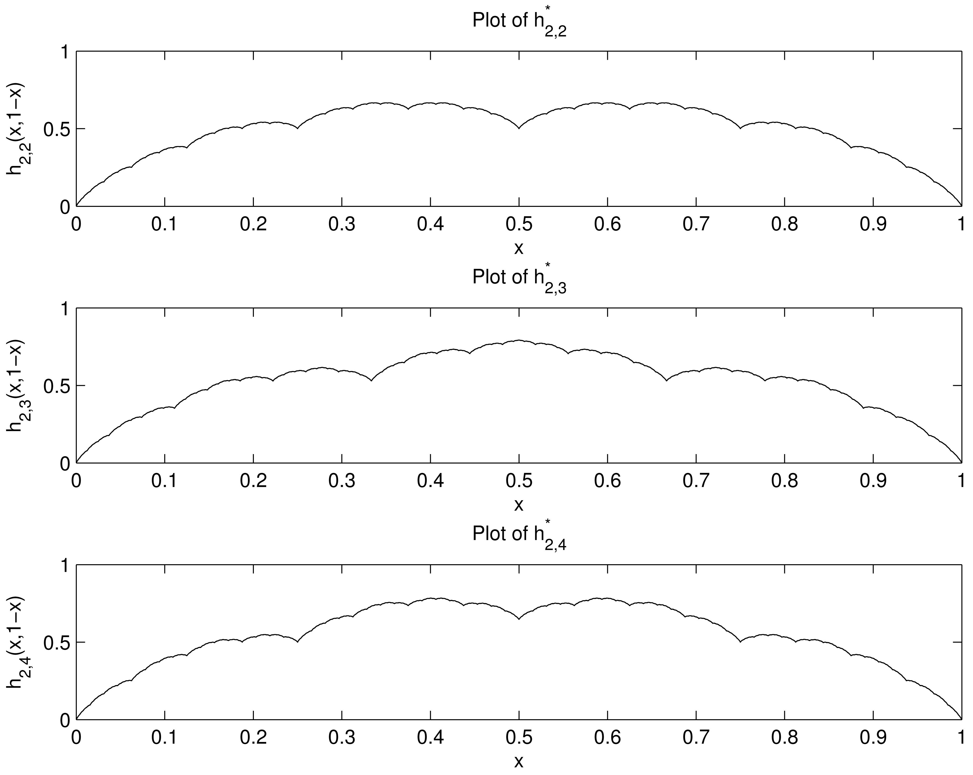
For each k ≥ 2, let be the function
We can obtain kn points on the plot of as follows. Let {Ti : i = 0, 1, …, k − 1} be the IFS on Ω2 given in Theorem 2, such that the attractor of this IFS is the graph of h2,k. Let S0(k) = {(0, 1, 0)}, and generate subsets S1(k), S2(k), …, Sn(k) of ℝ3 by the recursion
Then Sn(k) consists of kn points of the form (x, 1 − x, h2,k(x, 1 − x)). Projecting according to
The plot of used the set S24 (2), consisting of 224 = 16777216 points, computed in 4.2 seconds.
The plot of used the set S15 (3) consisting of 315 = 14348907 points, computed in 3.3 seconds.
The plot of used the set S12(4) consisting of 412 = 16777216 points, computed in 3.5 seconds.
We point out that the functions and , although their plots look similar, are not the same. For example, , whereas .
4. h3,k Is Self-Affine
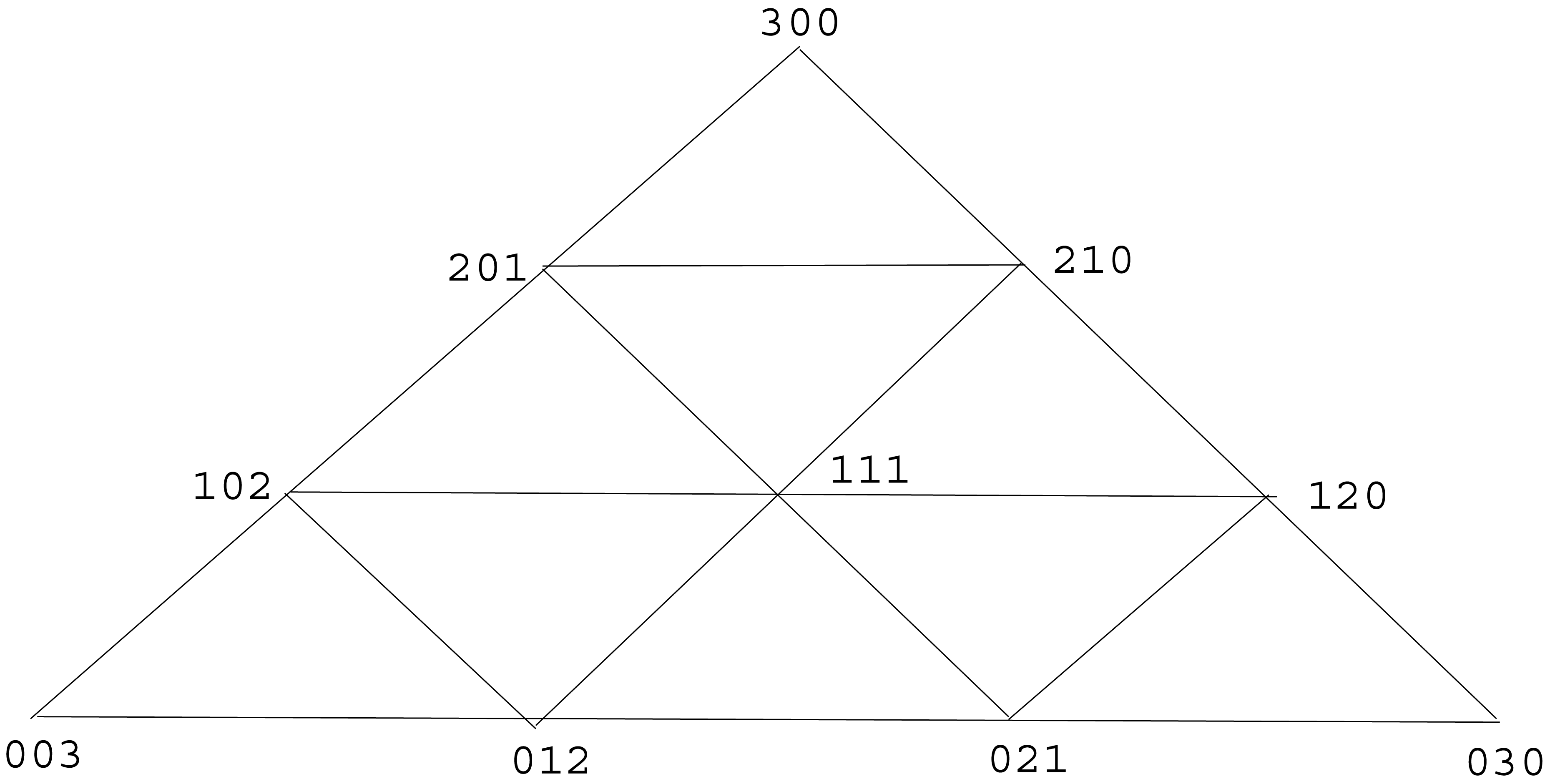
Fix k ≥ 2. It is the purpose of this section to study h3,k : ℙ3 → [0, ∞), the hierarchical entropy function induced by the unique finitary Λ(3, k)-indexed hierarchical source. In ℝ3, let Qk be the convex hull of the set {(k, 0, 0), (0, k, 0), (0, 0, k)}. Then Qk is an equilateral triangle whose three vertices are (k, 0, 0), (0, k, 0), (0, 0, k). We employ the well-known quadratic partition [7] of Qk into k2 congruent equilateral triangles, formed as follows. Partition each of the three sides of Qk into k line segments of equal length by laying down k − 1 interior points along the side. For each vertex of Qk, draw a line segment connecting the first interior points reached going out from the vertex along its two sides, then draw a line segment connecting the second interior points reached, and so forth until k − 1 line segments have been drawn. Doing this for each of the three vertices, you will have drawn a total of 3(k − 1) line segments, which subdivide Qk into the k2 congruent equilateral triangles of the quadratic partition. See Figure 3, which illustrates the quadratic partition of triangle Q3 into nine sub-triangles.
Let V1 be the set of all points (a, b, c) in Qk such that a is a positive integer and b, c are non-negative integers. There are k(k + 1)/2 points in V1. For each v = (a, b, c) in V1, let M1,v be the 3 × 3 matrix
For each v ∈ V1, the convex hull of the rows of M1,v is one of the sub-triangles in the quadratic partition of Qk, and these sub-triangles are distinct as v varies through V1. This gives us a total of k(k + 1)/2 of the sub-triangles in the quadratic partition of Qk, and we call these the V1 sub-triangles of the partition. Let V2 be the set of all (a, b, c) in Qk such that a is a non-negative integer and b, c are positive integers. There are k(k − 1)/2 points in V2. For each v = (a, b, c) in V2, let M2,v be the 3 × 3 matrix
For each v ∈ V2, the convex hull of the rows of M2,v is one of the sub-triangles in the quadratic partition of Qk, and these sub-triangles are distinct as v varies through V2. This gives us a total of k(k − 1)/2 of the sub-triangles in the quadratic partition of Qk, and we call these the V2 sub-triangles of the partition. The V1 sub-triangles are all translations of each other; the V2 sub-triangles are all translations of each other and each one can be obtained by rotating a V1 sub-triangle about its center 180 degrees, followed by a translation. Together, the k(k + 1)/2 V1 sub-triangles and the k(k − 1)/2 V2 sub-triangles constitute all k2 sub-triangles in the quadratic partition of Qk.
We define (k) to be the set of k2 matrices
Each row sum of each matrix in (k) is equal to k. Because of this property, we can define for each M ∈ (k) the mapping in which
Remarks
It is clear that the set of k2 mappings is an IFS on ℙ3. This fact allows one to prove (Lemma B.4 of Appendix B) that the related set of k2 mappings {TM : M ∈ (k)} is an IFS on Ω3. In the following example, we exhibit this IFS in a special case.
Example 5
Let k = 3. Referring to Figure 3, we see that the 9 matrices in (3) are
Following Equation (19), let vi ∈ ℙ3 be the vector whose components are the H3,3 entropies of the rows of Mi. Letting α = log2 3 and β = log2 6, Formula (7) is used to obtain
Following Equation (18), for each i = 1, 2, …, 9, let Ti : Ω3 → Ω3 be the mapping defined by
Theorem 3 which follows will tell us that the graph of h3,3 is the attractor of the IFS .
Theorem 3
Let k ≥ 2 be arbitrary The following statements hold:
(a): {TM : M ∈ (k)} is an IFS on Ω3.
(b): h3,k is self-affine and its graph is the attractor of the IFS in (a).
(c): For each M ∈ (k),
Our proof of Theorem 3 requires a couple of lemmas, which follow.
Lemma 3
Let λ ∈ Λ(3,k)+, let ϕ ∈ Φ(3,k) be the function given in Example 4, and let ϕ(λ) = (λ1, λ2, …, λk). Suppose we write
Proof
If each ri < k, then by definition of ϕ(λ) in Example 4, the properties Equations (21)–(23) are true. Now suppose at least one ri = k. Then exactly one ri = k (since otherwise some ri = 0, which is not allowed). By symmetry, we may suppose that r1 = k. We may now express λ as
Since r2, r3 ∈ {1, 2, …, k − 1}, and r2 + r3 = k, the definition of ϕ(λ) tells us that
Equation (24) yields Equation (23), Equation (25) yields Equation (22), and Equation (21) is vacuously true because k − r1 = 0.
Lemma 4
Let ϕ ∈ Φ(3, k) be the function given in Example 4. Properties (a.1)-(a.2) below are true for any matrix M in the set (k).
(a.1): If λ is a type in Λ(3, k), then λM ∈ Λ(3, k) and ‖λM‖ = k‖λ‖;
(a.2): If λ is a type in Λ(3, k)+, and ϕ(λ) = (λ1, λ2, …, λk), then ϕ(λM) is some permutation of (λ1M, λ2M, …, λkM).
Proof
Property (a.1), whose proof we omit, is a simple consequence of the fact that each matrix in (k) has row sums equal to k. Fix λ ∈ Λ(3, k)+ and fix M ∈ (k). Let r(λ) = (r1, r2, r3), and let
M is either of the form Equation (15) (Case 1) or of the form Equation (16) (Case 2). Throughout the rest of the proof, we employ the parameter β = (r1 + r2 + r3)/k. As remarked in Example 4, β ∈ {0, 1, 2}.
Proof for Case 1
We have , where
Note that
If β = 0, then
From Equation (26), we have , and therefore Property (a.2) follows. If β = 1, by definition of ϕ(λ) and ϕ(λM) in Example 4,
Property (a.2) then follows if the equations
Finally, if β = 2,
Property (a.2) then follows if the equations
Proof for Case 2
We have
Note that
If β = 0, then
From Equation (33), we have
In view of the fact that Equations (27–29) also hold, Property (a.2) then follows if the equations
Thus, Property (a.2) holds. Finally, suppose that β = 2. The entries of belong to {1, 2, …, k} and their sum is k. Under these conditions, no entry of can be equal to k, and so all entries belong to the set {1, 2, …, k − 1}. By definition of ϕ(λM) in Example 4,
In view of the fact that Equations (30–32) also hold, Property (a.2) then follows if the equations
Thus, Property (a.2) holds.
Proof of Theorem 3
We first derive part(c) and then part(b) (part(a) is already taken care of, as remarked previously). We derive part(c) by establishing Equation (20) for a fixed M ∈ (k). Let ϕ ∈ Φ(3, k) be the function given in Example 4 and recall that H3,k denotes the entropy function Hϕ on Λ(3, k). Referring to the definition of in Equation (17) and TM in Equation (18), we see that proving Equation (20) is equivalent to proving
We first show that
The proof is by induction on ‖λ‖. Equation (35) holds for ‖λ‖ = 1, which is the three cases λ = (1, 0, 0), λ = (0, 1, 0), λ = (0, 0, 1). Fix λ* ∈ Λ(3, k) for which ‖λ*‖ > 1, and for the induction hypothesis assume that Equation (35) holds when ‖λ‖ is smaller than ‖λ*‖. The proof by induction is then completed by showing that Equation (35) holds for λ = λ*. Let ϕ(λ*) = (λ1, λ2, …, λk). By the induction hypothesis,
Adding,
By Lemma 4, ϕ(λ*M) is a permutation of (λ1M, λ2M, …, λkM), and so by Equation (3),
It is easy to see that
Therefore,
Equation (34) then follows since the set is dense in ℙ3 and h3,k is a continuous function on ℙ3, completing the derivation of part(c) of Theorem 3. All that remains is to prove part(b) of Theorem 3. Letting G = {(p, h3,k(p)) : p ∈ ℙ3} be the graph of h3,k, part(c) is equivalent to the property that
Note that
5. Properties of Hierarchical Entropy Functions
We conclude the paper with a discussion of some properties of the self-affine hierarchical entropy functions h2,k and h3,k. For each m ∈ {2, 3} and each k ≥ 2, hierarchical entropy function hm,k obeys the following properties.
P1: hm,k is a continuous function on ℙm.
P2: If two probability vectors p1, p2 in ℙm are permutations of each other, then
P3: If p ∈ ℙm is degenerate (meaning that it is a permutation of the vector (1, 0, 0, …, 0)), then hm,k(p) = 0.
P4: For each p ∈ ℙm,
Properties P1-P4 are simple consequences of what has gone before. For example, to see why the symmetry property P2 is true, first observe that Hm,k(λ1) = Hm,k(λ2) if λ1, λ2 are types which are permutations of each other; this symmetry property for entropy on types then extends to ℙm using the fact that the finitary source which induces hm,k is entropy-stable.
The well-known Shannon entropy function hm on ℙm is defined by
The inequality


Acknowledgments
The work of the author was supported in part by National Science Foundation Grant CCF-0830457.
Appendix A
In this Appendix, we prove Theorem 1. In the following, the infinity norm ‖x‖∞ of a vector x = (x1, x2, …, xm) ∈ ℝm is defined as maxi |xi|.
Lemma A.1
Let be a function, and let
If , then f is uniformly continuous on .
Proof
We show there exists B > 0 such that
(p.1): For each j ≥ 0 and each pair of distinct types λ0, λ ∈ Λj(m, k), the following is true. Letting I = m‖λ0 − λ‖∞, there exist types λ1, λ2, …, λI in Λj(m, k) such that λI = λ and
(In other words, we can travel from λ0 to λ via a path in Λj(m, k) consisting of I terms, with successive terms no more than distance 1 apart in the infinity norm.)(p.2): There is a positive integer M for which the following is true. For each j ≥ 1 and each λ0 ∈ Λj(m, k), there exist types λ1, λ2, …, λM in Λj(m, k) such that λM/k ∈ Λj−1(m, k) and
(In other words, we can travel in Λj(m, k) from any type to a type divisible by k via a path consisting of M terms, with successive terms no more than distance 1 apart in the infinity norm.)
Let J ≥ 0. Suppose q1, q2 belong to and ‖q1 − q2‖∞ ≤ k−J. Fix J′ > J and types λ1, λ2 in ΛJ′(m, k) such that q1 = pλ1 and q2 = pλ2. Starting at λ1 and applying property (p.2) repeatedly (that is, for each j going backwards from j = J′ to j = J + 1), we obtain such that
Similarly, we find such that
By the triangle inequality, we have
Applying property (p.1),
Proof of Theorem 1
Let
= {S(λ) : λ ∈ Λ(m, k)} be a finitary hierarchical source. For every λ ∈ Λ(m, k), we have H(S(kλ)) = kH(S(λ)) and hence the normalized entropies H(S(kλ))/‖kλ‖ and H(S(λ))/‖λ‖ coincide. It follows that there exists a unique function
such that
It is easily seen that
is entropy-stable by the definition in Section 2.2 if f can be extended to a continuous function on ℙm (which will be the hierarchical entropy function induced by
). This extension will be possible if f is uniformly continuous on
, and we establish this by showing that Σj ∊j < ∞, where {∊j} is the sequence in Equation (38). Let ϕ ∈ Φ(m, k) be such that
ϕ =
. Let j ≥ 1 and let λ, µ be types in Λj(m, k) for which ‖λ − µ‖∞ ≤ 1. Letting
We conclude that
Appendix B
This Appendix proves some auxiliary results useful for proving Theorems 2–3. Henceforth, ‖x‖2 shall denote the Euclidean norm of a vector x in a finite-dimensional Euclidean space.
Lemma B.1
Let
be an IFS of contraction mappings on Ωm. Let π be the projection mapping (p, y) → p from Ωm onto ℙm. Suppose for each T ∈
, there is a contraction mapping T* on ℙm such that T*(p) = π(T(p, y)) for every (p, y) in Ωm, and suppose ℙm is the attractor of the IFS {T* : T ∈
}. Suppose h : ℙm → ℝ is a continuous mapping whose graph Gh = {(p, h(p)) : p ∈ ℙm} satisfies the property
Then Gh is the attractor of
.
Proof
Let Q be the attractor of
. Since each mapping in
maps the compact set Gh into itself, Q ⊂ Gh by uniqueness of the attractor. The proof is completed by showing the reverse inclusion Gh ⊂ Q. Since π(Q) is the attractor of the IFS {T* : T ∈
}, we must have π(Q) = ℙm by assumption. Let (p, h(p)) be an arbitrary element of Gh. Since π(Q) = ℙm, there exists a point in Q of the form (p, y). But (p, y) and (p, h(p)) both belong to Gh, so y = h(p). We conclude (p, h(p)) belongs to Q, and therefore Gh ⊂ Q.
Lemma B.2
Let T* : ℙm → ℙm be a contraction mapping with contraction coefficient σ ∈ (0, 1), meaning that
Let c = (c1, c2, …, cm) be a vector in ℝm and define its variance by
Then T is a contraction mapping if V(c) < σ−2(1 − σ2)2.
Proof
By the intermediate value theorem, there is a real number λ in the interval [σ, 1) such that
Then T is a contraction if we show that
The right hand side of Inequality (42) is equal to
Therefore, we will be done if we can show that
It follows that Inequality (43) will be true for all p, q, u, v if
It is a simple exercise in Lagrange multipliers, which we omit, to show that the vector x = (x1, …, xm) satisfying the constraints in Equation (44) which maximizes the dot product x · c is the vector for which
For this choice of x, x · c can be seen to be . Therefore, we will be done if
But this is true with equality, by Equation (41).
Lemma B.3
Let k ≥ 2 be arbitrary. Then, for each i = 0, 1, …, k − 1, the mapping Ti : Ω2 → Ω2 defined in Section 3 is a contraction.
Proof
Fix i in {0, 1, …, i − 1}. The mapping is a contraction mapping with contraction coefficient k−1. Applying Lemma B.2 with σ = k−1, Ti will be a contraction mapping if we can show that
It is easy to compute that
Using the fact that
Choosing the smallest value of γ for which
Using calculus, it is easy to show that
Thus, Inequality (45) holds, and our proof is complete.
Lemma B.4
Let k ≥ 2 be arbitrary. Then, for each matrix M in the set of matrices (k), the mapping TM : Ω3 → Ω3 defined in Section 4 is a contraction.
Proof
The mapping is a contraction with contraction coefficient k−1. Applying Lemma B.2 with σ = k−1, we have to show that various variances are all less than (k − k−1)2. Specifically, for each (a, b, c) ∈ V1 we wish to show
Using Formula (7), the variance on the left side of Inequality (47) is equal to
Let a1 = a, a2 = b + 1, a3 = c + 1. For any constant γ satisfying 0 < γ < 1, we have
Using the fact that
Choosing the smallest value of γ for which
Similarly, the variance on the left side of Inequality (48) is V(log2(a + 1), log2 b, log2 c), and
Using calculus, it is easy to show that
Thus, for each (a, b, c) ∈ V1, we have the desired inequality
References
- Csiszár, I.; Körner, J. Information Theory: Coding Theorems for Discrete Memoryless Systems, 2nd ed.; Cambridge University Press: Cambridge, UK, 2011. [Google Scholar]
- Kieffer, J. Hierarchical Type Classes and Their Entropy Functions. Proceedings of the 1st International Conference on Data Compression, Communication and Processing, Palinuro, Campania, Italy, 21–24 June 2011; pp. 246–254.
- Oh, S.-Y. Information Theory of Random Trees Induced by Stochastic Grammars. Ph.D. Thesis, University of Minnesota Twin Cities, Department of Electrical & Computer Engineering, Minneapolis, MN, USA, 2011. [Google Scholar]
- Brualdi, R. Algorithms for constructing (0,1)-matrices with prescribed row and column sum vectors. Discret. Math. 2006, 306, 3054–3062. [Google Scholar]
- Fonseca, C.; Mamede, R. On (0,1)-matrices with prescribed row and column sum vectors. Discret. Math. 2009, 309, 2519–2527. [Google Scholar]
- Falconer, K. Fractal Geometry; John Wiley & Sons: Hoboken, NJ, USA, 2003. [Google Scholar]
- Soifer, A. How Does One Cut a Triangle? Springer-Verlag: Berlin, Heidelberg, Germany, 2010. [Google Scholar]
© 2011 by the author; licensee MDPI, Basel, Switzerland. This article is an open access article distributed under the terms and conditions of the Creative Commons Attribution license (http://creativecommons.org/licenses/by/3.0/.)
Share and Cite
Kieffer, J. A Catalog of Self-Affine Hierarchical Entropy Functions. Algorithms 2011, 4, 307-333. https://doi.org/10.3390/a4040307
Kieffer J. A Catalog of Self-Affine Hierarchical Entropy Functions. Algorithms. 2011; 4(4):307-333. https://doi.org/10.3390/a4040307
Chicago/Turabian StyleKieffer, John. 2011. "A Catalog of Self-Affine Hierarchical Entropy Functions" Algorithms 4, no. 4: 307-333. https://doi.org/10.3390/a4040307