Radio Frequency Interference Detection and Mitigation Algorithms Based on Spectrogram Analysis


Abstract
: Radio Frequency Interference (RFI) detection and mitigation algorithms based on a signal's spectrogram (frequency and time domain representation) are presented. The radiometric signal's spectrogram is treated as an image, and therefore image processing techniques are applied to detect and mitigate RFI by two-dimensional filtering. A series of Monte-Carlo simulations have been performed to evaluate the performance of a simple thresholding algorithm and a modified two-dimensional Wiener filter.1. Introduction
Microwave radiometry is today routinely used to remotely measure geophysical parameters. Microwave radiometers are highly sensitive instruments, but measurements may be corrupted by the presence of Radio-Frequency Interference (RFI). Sources of RFI include spurious signals and harmonics from lower frequency bands, spread-spectrum signals overlapping the “protected” band of operation, or out-of-band emissions not properly rejected by pre-detection filters.
The presence of RFI in the pre-detected voltage signal modifies the value of the measured power leading to an erroneous retrieval of the measured geophysical parameters [1–3]. In recent years, techniques to detect the presence of RFI in radiometric measurements have been developed. They include time- and/or frequency domain analyses [4], or statistical analysis of the received signal [5,6]. In addition, the so-called Spectral Kurtosis algorithm has been studied in [7] with good results, taking advantage of the effectiveness of the combination of different RFI detection algorithms.
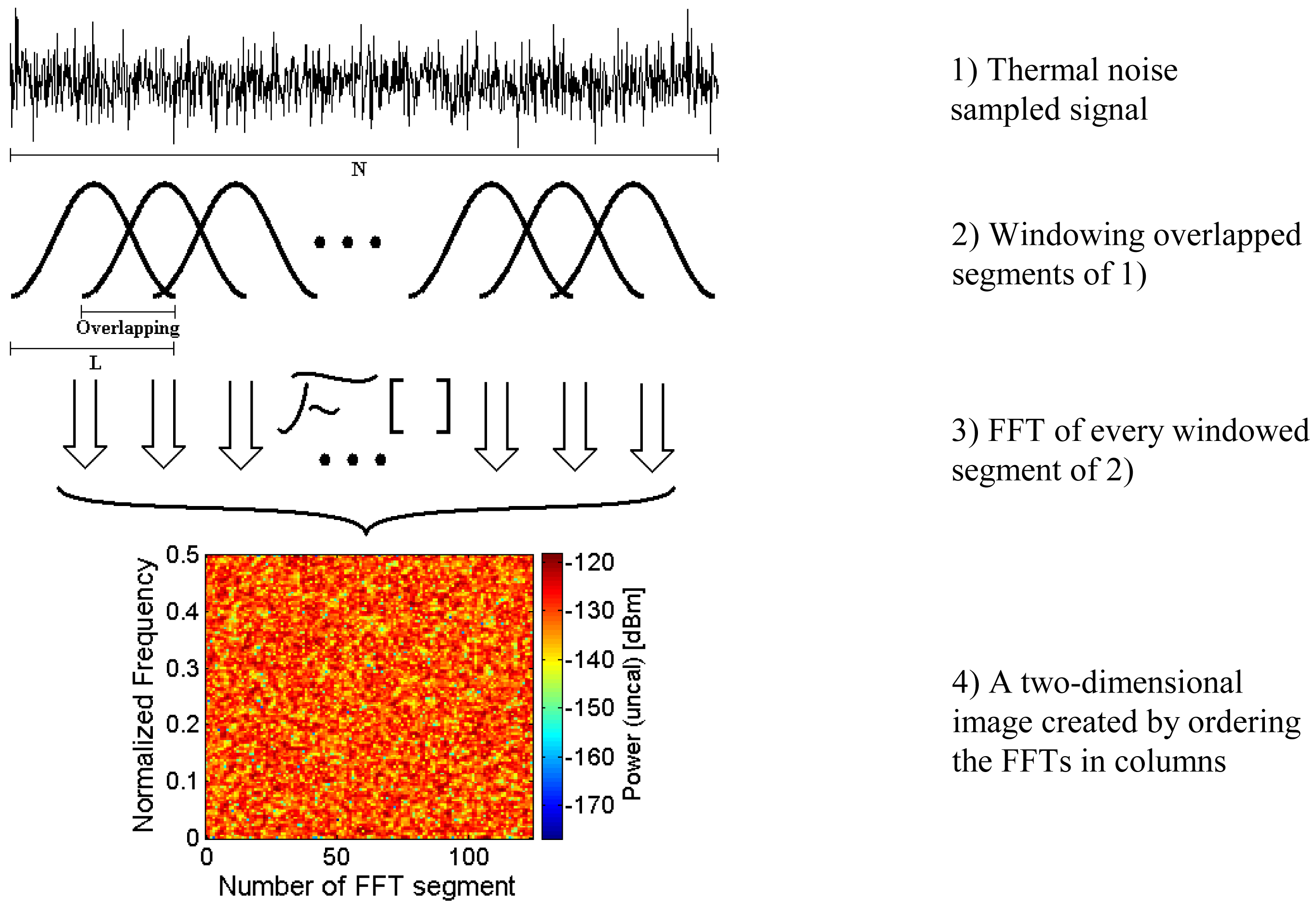
Combining the time and frequency domains analysis jointly, the spectrogram stands as a powerful tool which has been previously used in RFI detection in radio-astronomy [8,9]. The spectrogram consists of an intensity plot (usually on a decibel scale) of the Short-Time Fourier Transform (STFT) magnitude [10]. The STFT consists of a set of Fourier Transforms (FT) of consecutive windowed data segments from a longer data set. Windows usually overlap in time, thus data segments may have redundant information, as sketched in Figure 1. The STFT provides time-localized spectral information of the frequency components of a signal varying over time, whereas the standard FT provides the frequency information averaged over the entire signal time interval [10]. As a spectrogram is a two-dimensional intensity plot, it can be analyzed as an image, thus having all the image processing tools at our hand.
In this work, a simple thresholding algorithm to detect and eliminate interference patterns in radiometric signal spectrograms is developed first, and simulation results are presented. The simulated RFI signals are generically from the sinusoidal and chirp families. By adjusting the signals' parameters, the bandwidth and temporal duration, many different types of signals can be obtained. A two-dimensional (2D) Wiener filter is then applied to the spectrogram in order to try to improve the cancellation of RFI components in the radiometric signal. A brief description of the spectrogram calculation is given in Section 2. Section 3 describes the image processing algorithm proposed in this work, which is called “Smoothing Algorithm”. In Section 4 the Wiener filtering process is described and compared to the “Smoothing Algorithm” proposed. Section 5 shows the results obtained with the application of both algorithms to a thermal noise signal contaminated with a set of RFI chirp signals. Finally, Section 6 summarizes the conclusions of this work.
2. Spectrogram Calculation
In this work, radiometric signals are assumed to be sampled at an adequate sampling rate satisfying the Nyquist criterion and the spectrograms are obtained from these discrete time signals.
The spectrogram calculation depends on several parameters which are: the total number of signal samples, the FFT size, the window used for the FFT calculation of the data segments, and the overlapping between these data segments, as shown in Figure 1.
The spectrogram used in this paper is calculated using discrete samples, each one corresponding to a measurement of the pre-detected voltage signal. The number of samples (N) which forms the spectrogram will determine the radiometric resolution obtained by each spectrogram.
The FFT size is the number of samples used to compute each FFT and determines the spectral and temporal resolutions. If the FFT size (L) increases, the spectral resolution increases, while the temporal resolution decreases, since the time lapse between consecutive data segments increases. In contrast, smaller FFT sizes lead to lower frequency resolution, and higher temporal resolution. Therefore, selection of the FFT size must be chosen carefully depending on the RFI present in the radiometric measurements.
The FFT calculation requires the use of an analysis window function in order to minimize unwanted “side lobes” and ringing in the FFT resulting from abrupt truncations at both ends of the data segment. This situation causes an oscillatory behavior in the FFT called the Gibbs phenomenon [11]. Several functions can be used to avoid this problem, though when the data source is unknown, the Hann window is one of the most common windows used in spectrum analysis because of its excellent roll-off rate at 18 dB/octave [12].
In order to avoid loss of data when using a window in the FFT calculation, some overlapping (O) must exist between consecutive data segments (Figure 1). In addition, overlapping increases the temporal resolution as the beginning of the data segments is reduced. However, increasing the overlap leads to an increase of the total number of samples to be computed and managed, complicating the hardware design. Overlap factor is recommended to be 75% for a Hann window [13,14]; in this work a value of O = 75% is used.
The spectrograms calculated in this work have the following parameters:
Number of samples: this parameter must be as high as possible to maximize the radiometric resolution, as a higher number of samples means a longer integration time. On the other hand too large values increase the computation time required to perform the Monte-Carlo simulations. The value chosen in this work is N = 218 samples.
Overlap: for the case of 218 samples, an overlap value of O = 75% is reasonable [13,14] to avoid information loss.
FFT size: The FFT size determines the frequency resolution and the number of FFT segments, determines the temporal resolution. For the simulations performed in this work, and supposing that any information of the RFI is known, the FFT size was chosen to be equal to the number of FFT segments, to have similar spectral and temporal resolutions (both resolutions may not be the optimal ones); thus the FFT size should be the square root of the number of samples (N). Taking into account that there exists a 75% overlap between consecutive Hann windows, the number of FFT segments has to be multiplied by 4. Thus, to equilibrate both resolutions, maintaining the original compromise, the FFT size has been selected to be L = 210, and now the total number of samples is 220 (accounting redundant points due to overlapping).
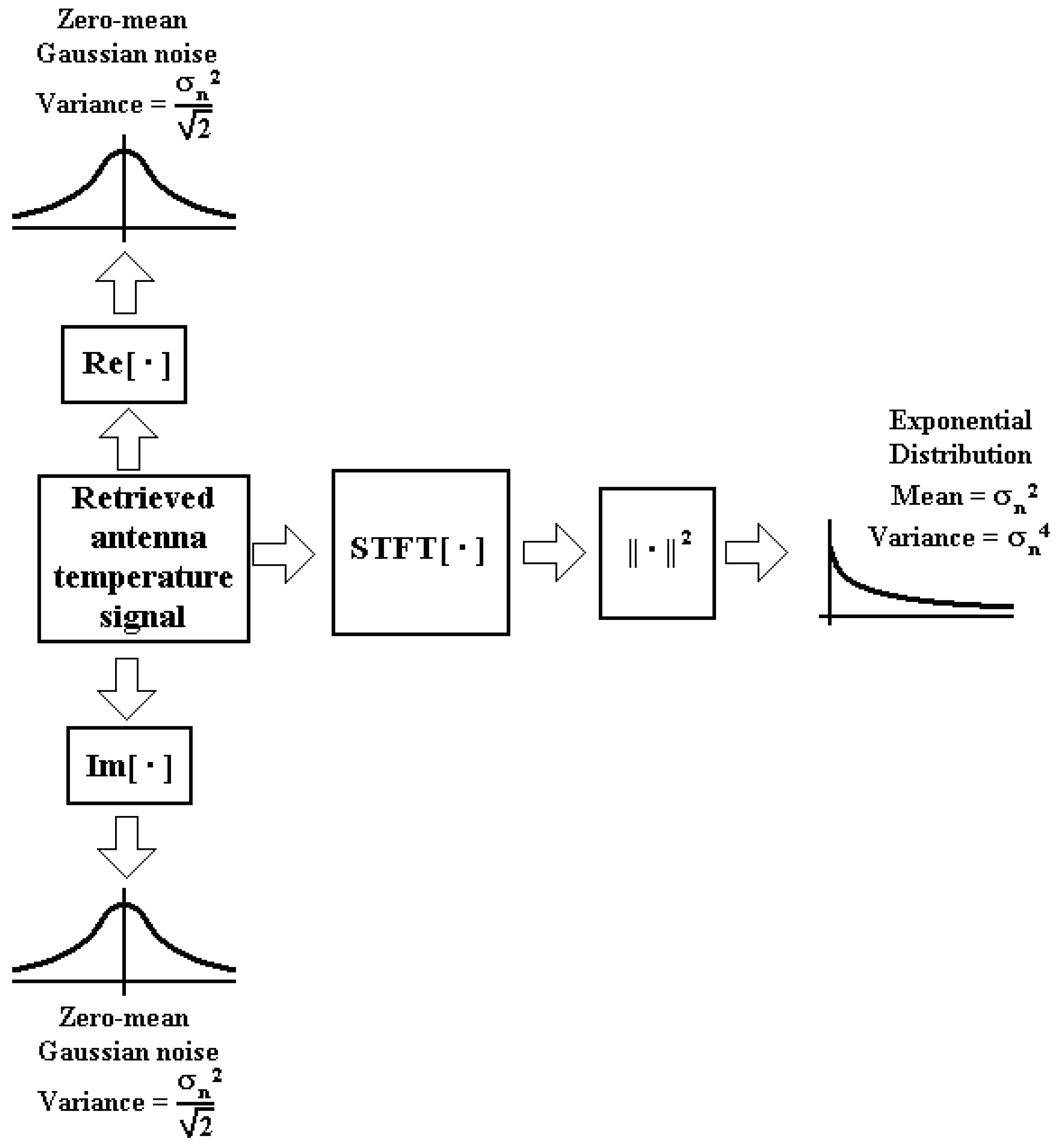
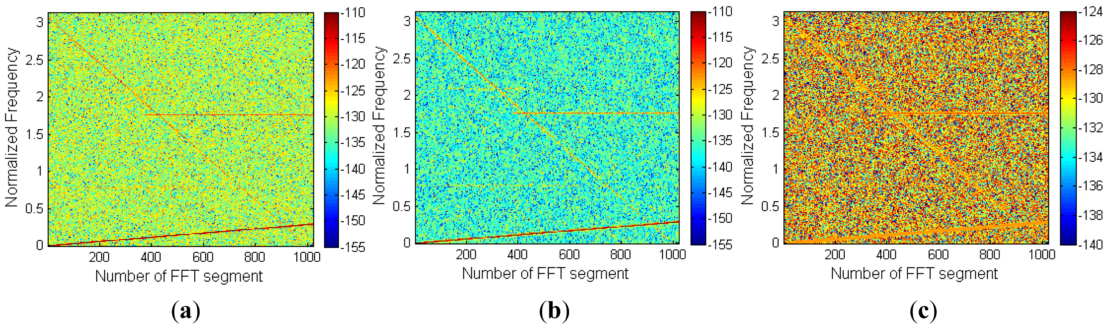
As it has been said, the spectrogram operation consists of the power (square of the absolute value) of the STFT magnitude. The spectrogram operation changes the probability density function of the received thermal noise which is a pair of Gaussian distributed random variables (one for the in-phase component and the other one for the quadrature component). The square of the amplitude is equal to the sum of the squares of both Gaussian distributions, which is the definition of a chi-square distribution with two degrees of freedom, which is equivalent to an exponential distribution [15]. Figure 2 sketches this process.
3. Smoothing Algorithm
The most obvious way to detect the presence of interference in a radiometric signal is by detecting power peaks in the received signal that are larger than the variance of the measured thermal noise in the absence of RFI. This detection can be performed either in both the time and frequency domains.
This technique can be straight-forwardly extended to the spectrogram. Considering that a power peak is produced by an RFI signal, the threshold value must be a function of the thermal noise variance (power), and must maximize the probability of RFI detection (Pdet) and minimize the probability of false alarm (Pfa) detection. RFI probability of detection cannot be computed in advance since the presence of RFI is unknown, but the probability of false alarm is easy to obtain as the thermal noise follows a known Gaussian distribution.
All simulations performed in this work have been performed assuming an antenna temperature (TA) of 300 K and a radiometer receiver noise temperature of 100 K. In order to make a relationship between the noise power and the RF interfering signal power, the Interference-to-Noise Ratio (INR) is defined as:
The threshold value of this algorithm must be selected to limit the error in the estimated antenna temperature produced by false alarms.
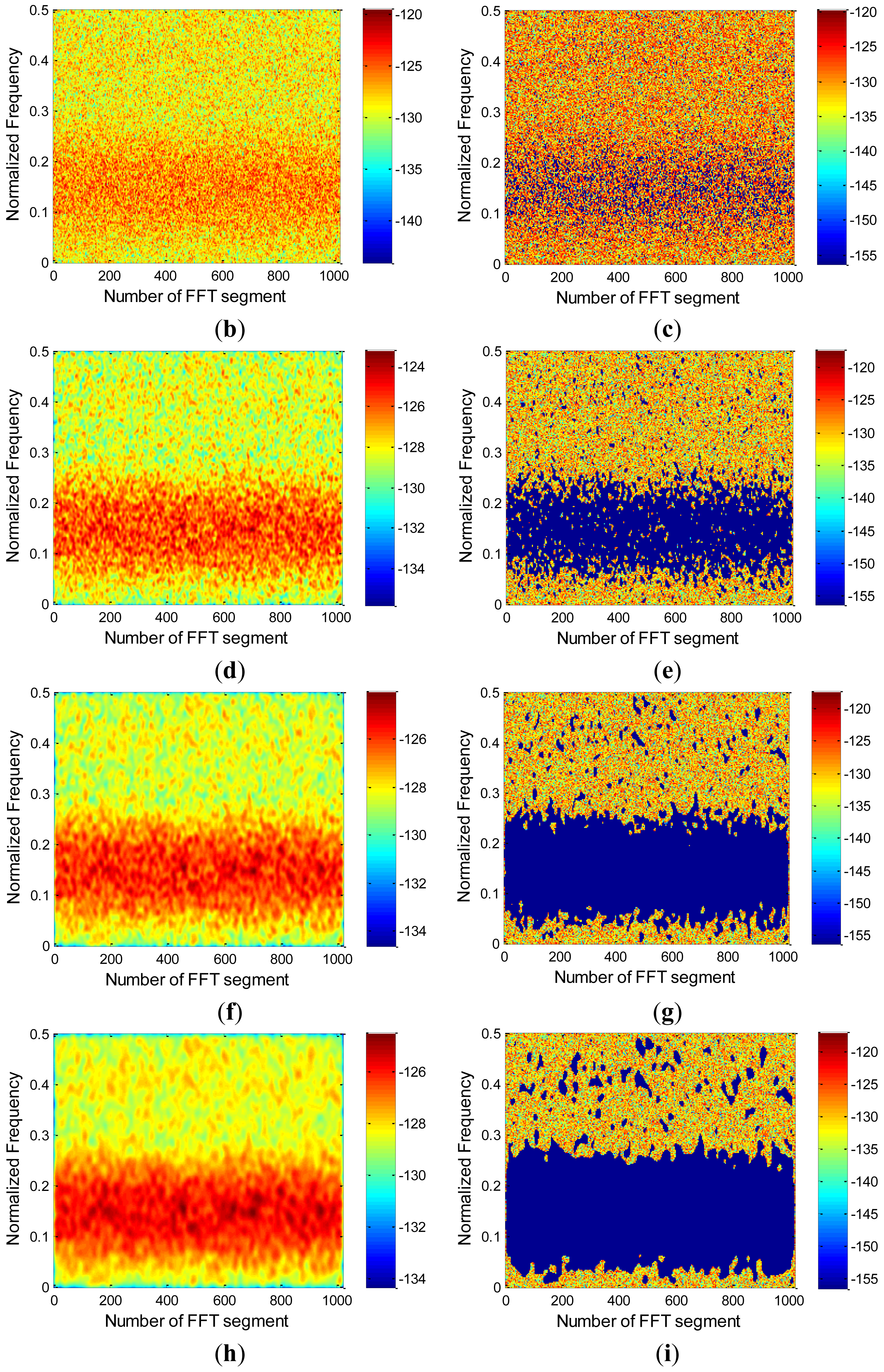
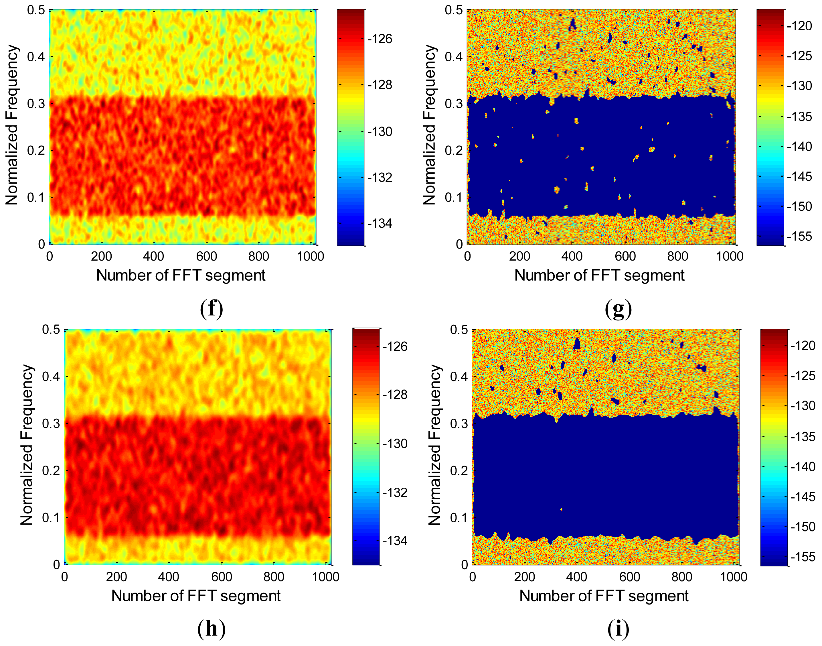
If an RFI-free spectrogram is observed (Figure 1, panel 4) it is obvious that the noise power peaks are scattered (and usually isolated) in both frequency and time, while in an RFI contaminated spectrogram (e.g., Figure 4a), the RFI is usually clustered in determined regions in the frequency-time plane. Considering the spectrogram as an image, noise power peaks present higher spatial frequency contents (rapid variations) than the RFI, which are usually clustered. Hence, applying a 2D smoothing filter (low-pass filter) will attenuate these exponential “peaks”, while the RFI contaminated regions will be preserved. RFI is preserved so it can be detected with a more restrictive threshold.
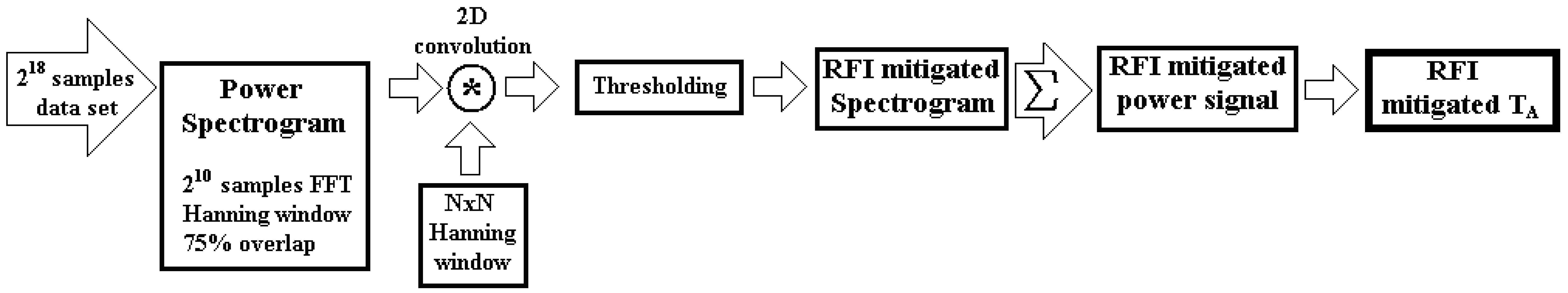
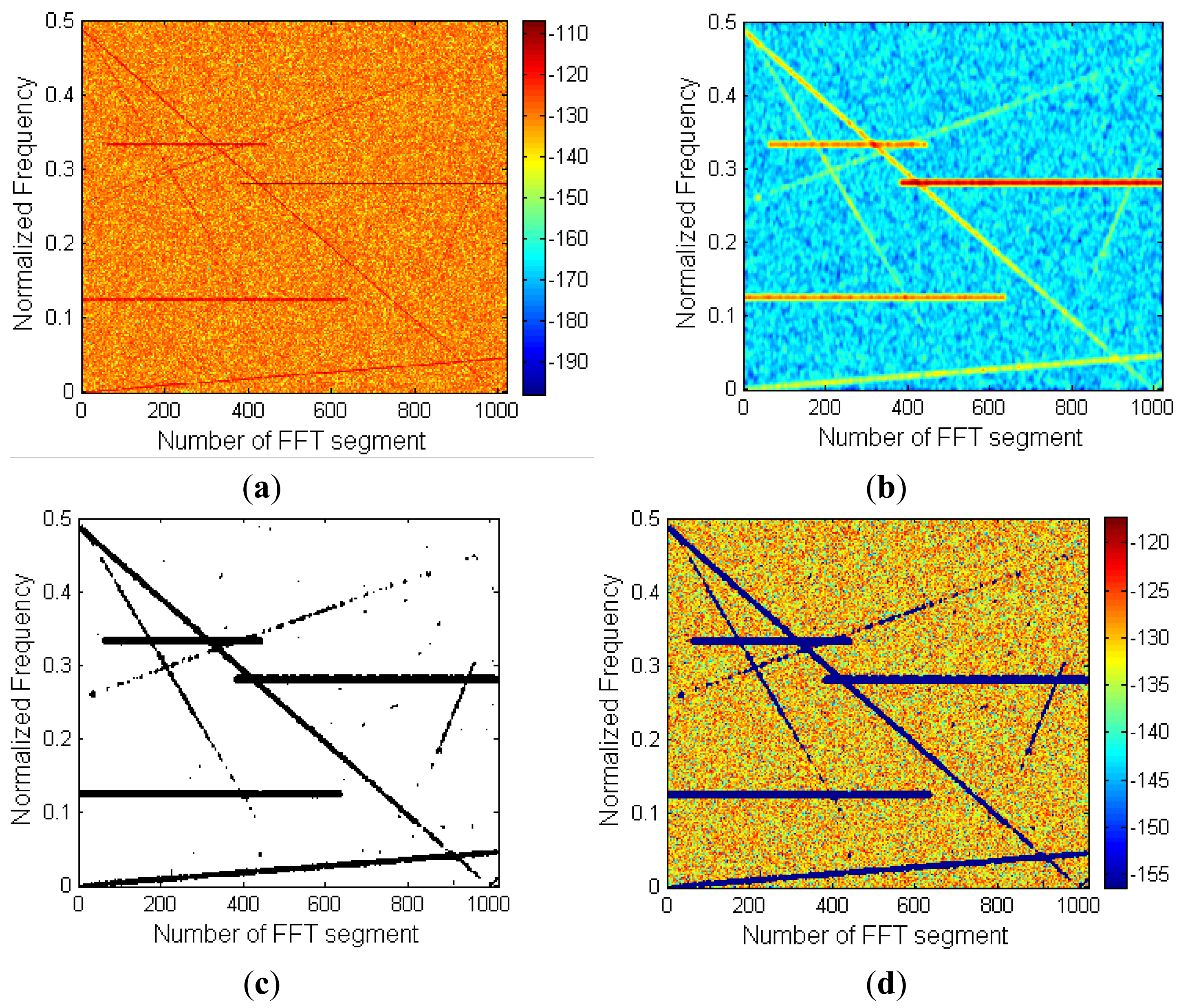
The algorithm proposed in this work can be summarized as follows with the aid of Figures 3 and 4:
Power spectrogram calculation of a data segment of 218 samples using data segments of 210 samples, with 75% overlap, and a Hann window (Figure 4a).
Convolution of the power spectrogram with a 2D low pass filter of a determined size (in this work the Hann window has been chosen, although a Gaussian or a Hamming window would perform similarly (see Figure 4b)).
Thresholding: a threshold is used in the smoothed power spectrogram, in order to detect clusters of RFI-contaminated pixels (Figure 4c). The optimum threshold will be discussed in Section 5.
Antenna noise power is calculated by averaging all spectrogram pixels below the threshold.
Finally, TA is obtained from the antenna noise power.
4. Wiener Filtering
As already discussed, the spectrogram of a noise signal with sinusoidal interference signals can be considered as a noisy image, where the noise is the spectrogram of the radiometric signal (the one we want to measure), and the image to be detected is the spectrogram of the interference (the one to be cancelled). Therefore, designing a filter to eliminate the noise from the image is the way to estimate the RFI, for a later removal of the interference without loss of the radiometric data.
The Wiener filter is a well-known adaptive filter used in communications, which provides the best estimation of a signal, equalizes communications channel, and eliminates the noise present in the received signal. In this section the Wiener filter is used to estimate the RFI in the spectrogram image, for a later cancellation and its performance is compared to the smoothing algorithm.
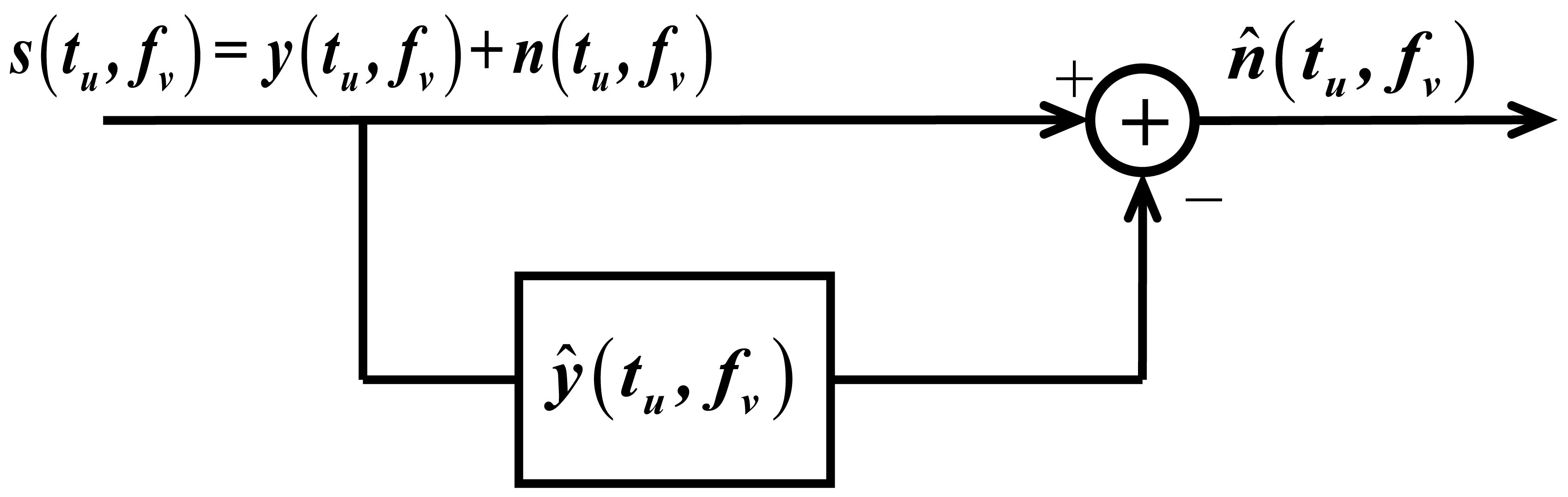
In our case of study, it is not necessary to know the effect of the communications channel in the spectrogram, thus, it will only be necessary to differentiate between the noise and the interfering signal. The way to perform this task is by using a locally adaptive linear minimum mean square error (LLMMSE) [16] to estimate the interfering signal's spectrogram.
The LLMMSE algorithm consists of an optimal linear estimator of our interfering signal ŷ(tu, fv) in combination with additive noise.
The minimum error (ε) is found for:
From Equations (4), (5.1) and (5.2), and taking into account that the additive noise power of the spectrogram does not have a zero mean, Equation (6) can be derived:
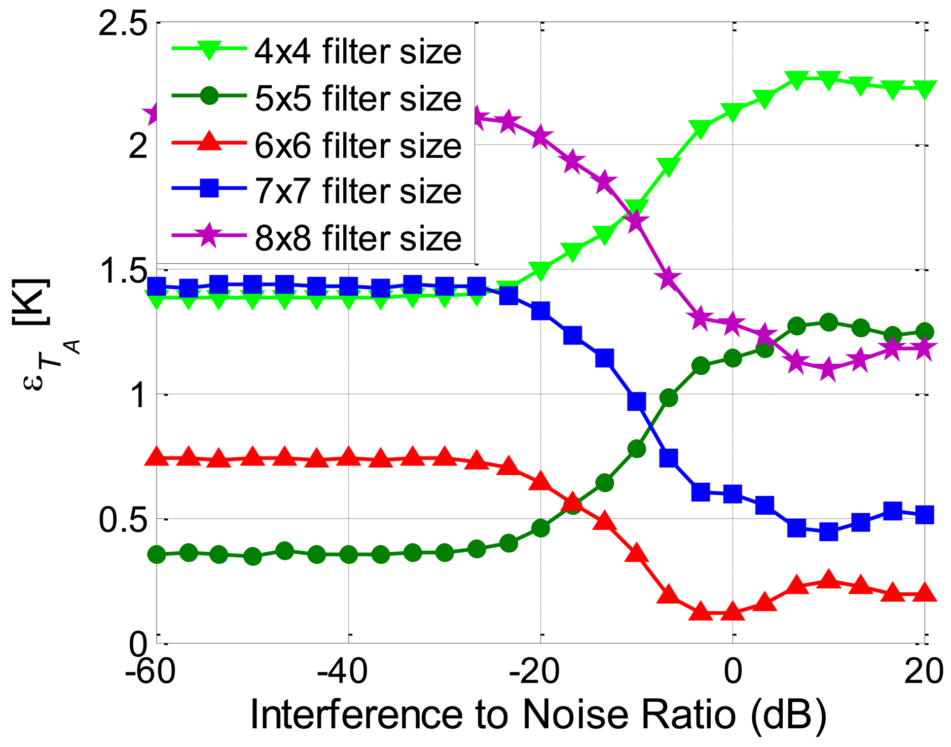
The use of different window sizes (L value, M1 + M2 + 1 = L) affects the resulting estimated interference ŷ(tu, fv). If L is too small, the noise filter algorithm is not effective. On the other hand, if L is too large subtle details of the interference will be lost in the filtering process. Figure 6 shows the simulated error in the estimation of the noise power as a function of the RFI power present in the received signal; assuming that the thermal noise power (σn2) is perfectly known. It is observed that the value of L depends on the actual RFI level: if the RFI level is 17 dB lower than the thermal noise, the best choice is a 5 × 5 window, otherwise, a 6 × 6 window will outperform. In our case of study, the 6 × 6 window is chosen as the maximum value of the algorithm error is 0.74 K.
5. Results
In this section, results obtained with the two image processing algorithms presented (Smoothing and thresholding and 2D Wiener filtering) are shown and discussed.
5.1. Smoothing Algorithm
5.1.1. Smoothing Algorithm Applied with Pulsed Sinusoidal and Chirp RFI
The use of the FFT implies that the Smoothing Algorithm is implicitly searching for sinusoidal interferences [5–7], therefore, in order to determine the correct performance of this algorithm, it has been tested with a set of linear chirp and sinusoidal interfering signals as defined in Equation (11).
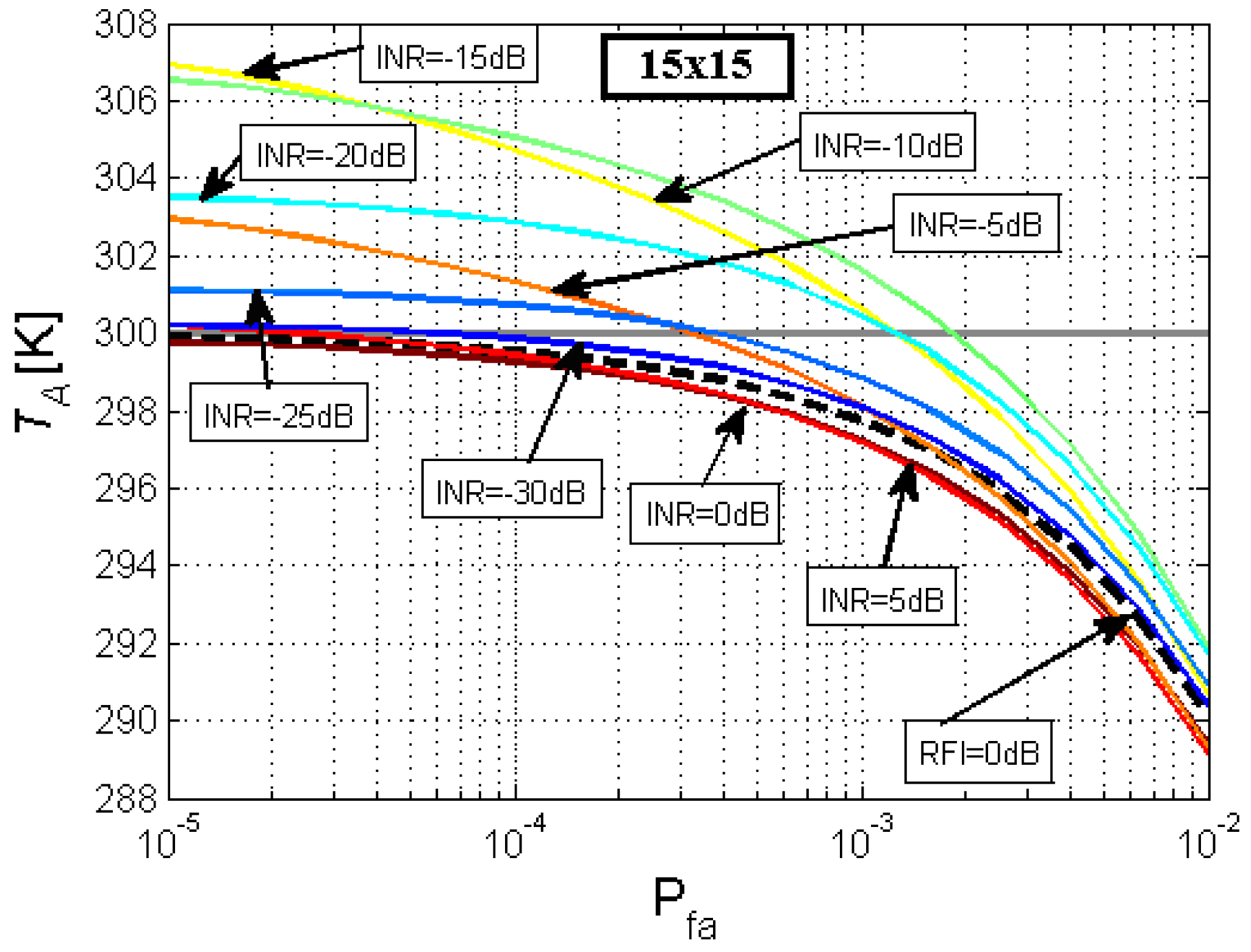
The retrieved error in TA as a function of the threshold's Pfa, the size of the smoothing filter and the power of the interfering signal is presented in Figures 7–9. To test the performance of the Smoothing Algorithm, a 15 × 15 Hann window is selected. Retrieved TA and error in the retrieved TA as a function of the threshold's Pfa are represented in Figures 8 and 9, respectively. Figure 7 shows the retrieved TA [K], for different interfering signal power (and even with no interference, black dotted line), with a fixed smoothing filter size (in this case a 15 × 15 Hann window), as a function of the Pfa of the threshold used in our algorithm. The TA value is obtained by means of 1024 Monte Carlo simulations on a Pentium D at 3.4 GHz with 2 GB of RAM. Simulation time (16 Pfa levels and 9 INR levels) was 3 h and 5 min. The actual TA value is 300 K which is asymptotically achieved by the black dotted line (in abscense of RFI) as Pfa decreases. As it can be seen, the selection of the Pfa threshold is crucial, as a low Pfa values decreases the probability of detection of RFI-contaminated pixels, leading to a retrieved temperature higher than the real antenna temperature. On the other hand, a high Pfa value will produce a high number of false alarms which will produce a clipping in the probability distribution function of the power spectrogram pixels, leading to a retrieved TA lower than the real antenna temperature.
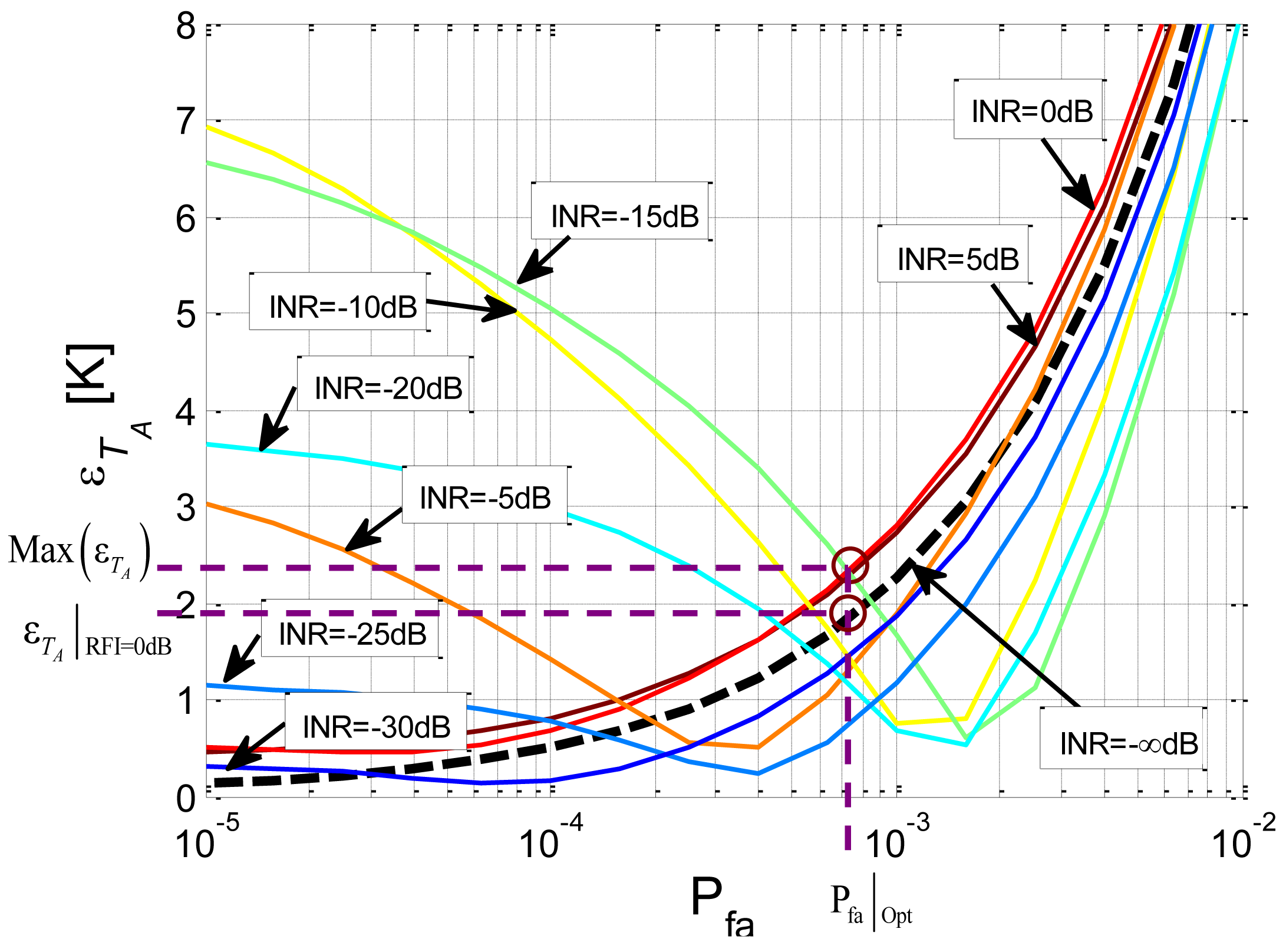
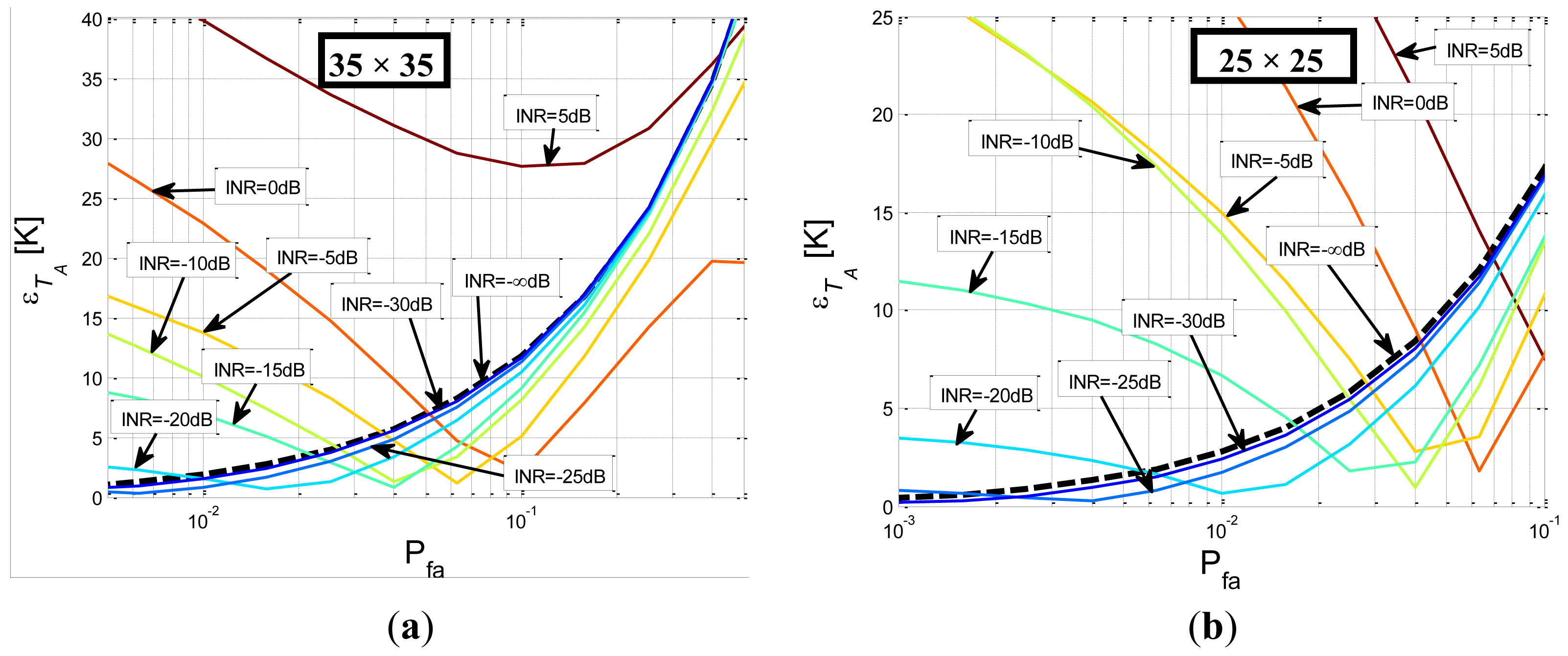
In Figure 8, the error introduced by the Smoothing Algorithm in the retrieved antenna temperature εTA [K] is represented for different interfering signal powers, with a fixed smoothing filter size: (15 × 15 Hann window). It can be observed that RFIs with high INR values are accurately eliminated with a threshold with a low Pfa, while in the case of RFIs with INR value between −5 dB and −25 dB applying a low threshold leads to an important error produced by the fact that a great part of the RFI contaminated pixels “pass under” the threshold with low Pfa. The selection of the Pfa threshold is a compromise between a not too high value to clip the power PDF (Pfa > 7.24·10−4 in Figure 8, INR = 0 dB) and not too low to leave a high rate of undetected RFI contaminated pixels (Pfa < 7.24·10−4 in Figure 8, INR = −15 dB).
Combining different simulations with RFIs of different powers (INR from 5 dB to −30 dB compared to the noise power) it is observed that the threshold with optimum performance has a Pfa ∼ 7.24 ×·1 0−4 (Pfa|Opt in Figure 8) with a maximum RMS error value of 2.33 K (Max(εTA) in Figure 8), and RMS error value without RFI of 1.84 K (εTA|RFI=0dB in Figure 8) which it will be the error obtained in case of RFI free situation; the threshold value associated to Pfa|Opt is equal to 1.37·σ2n.
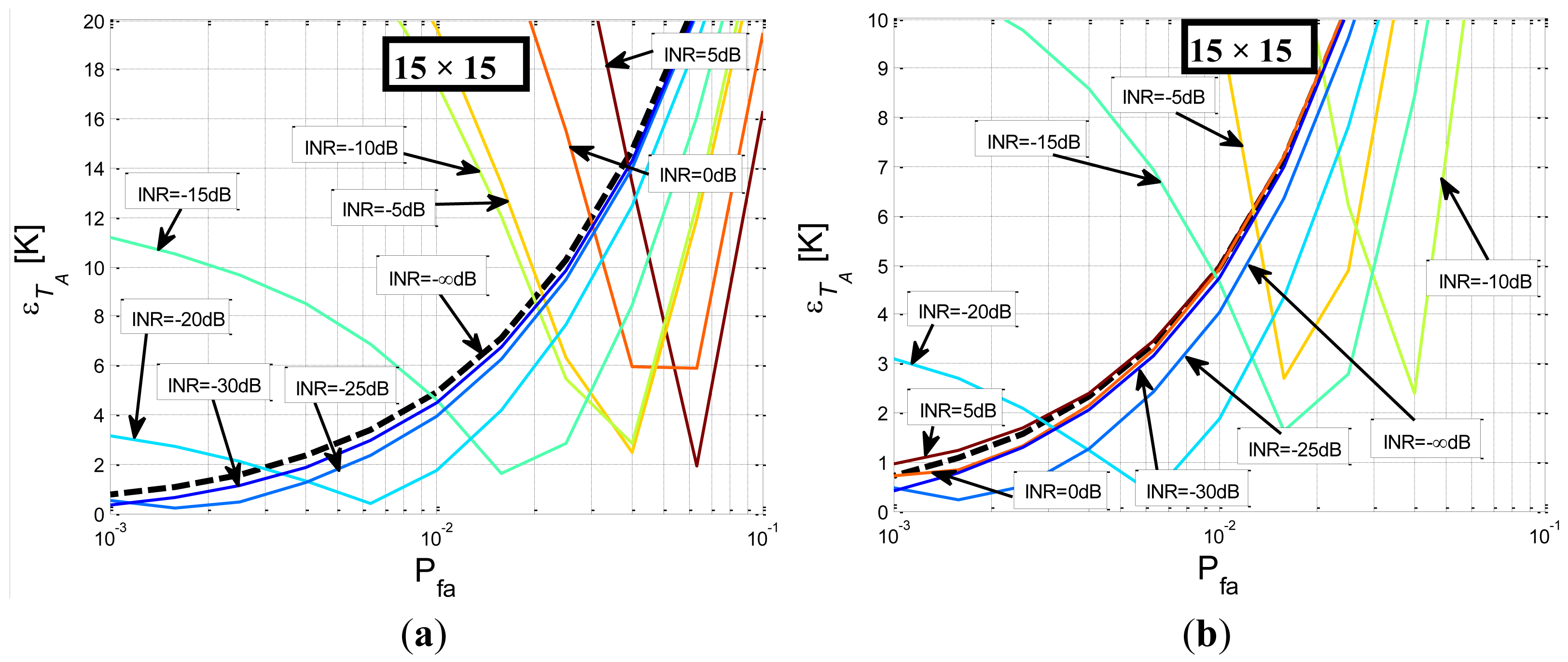
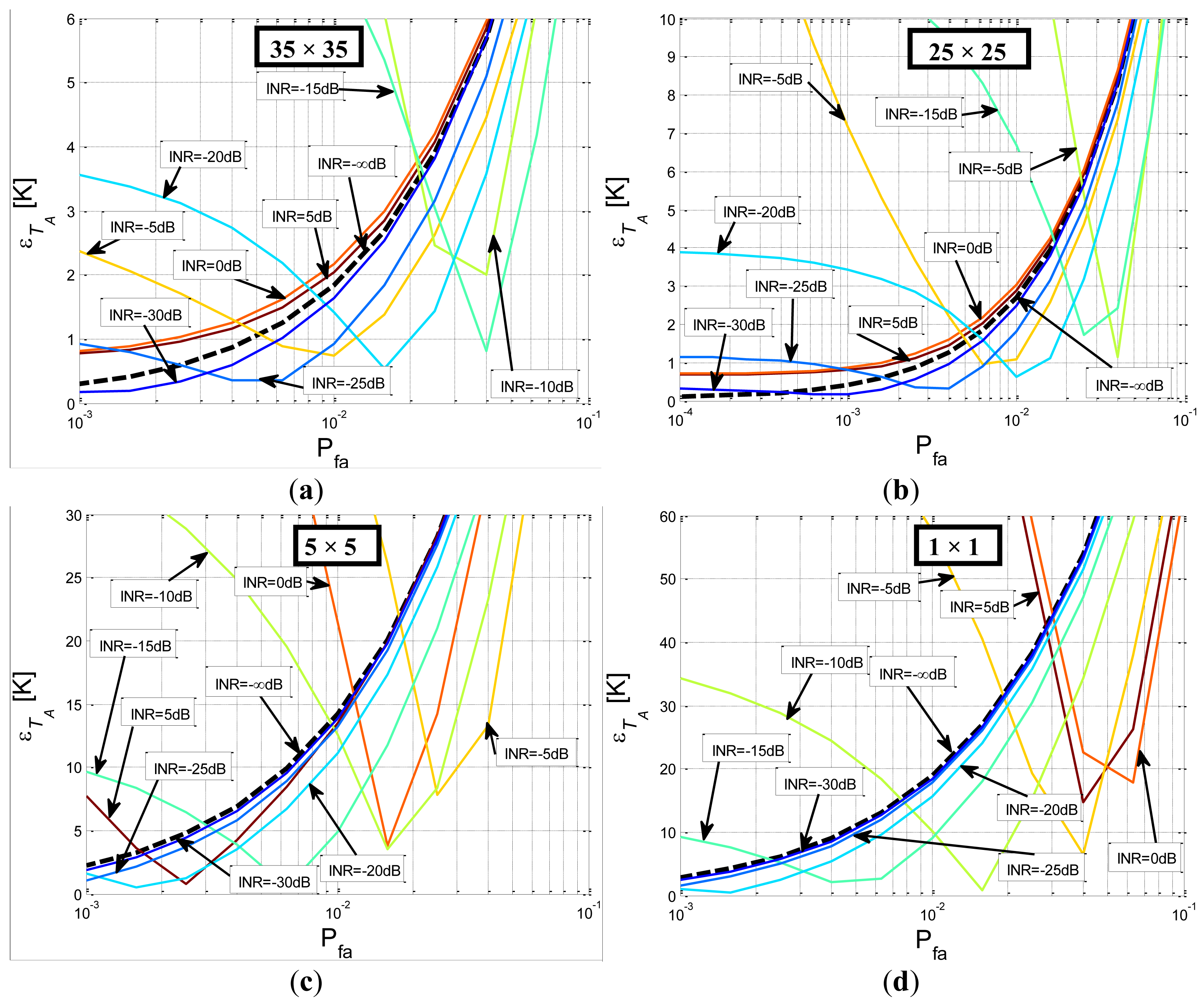
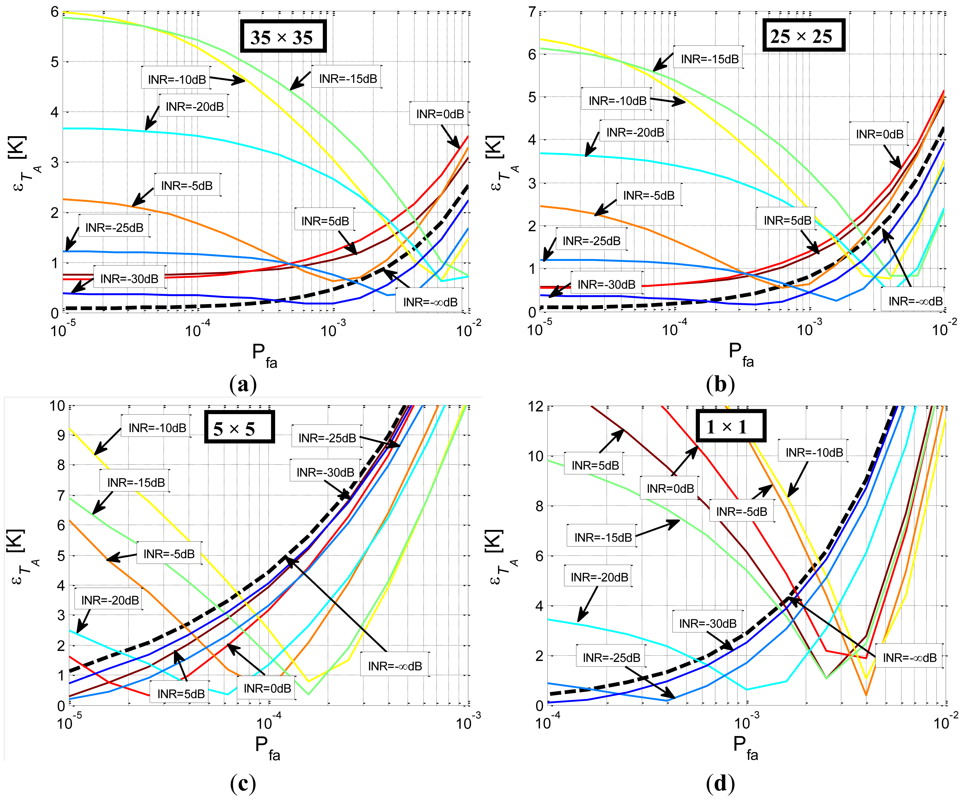
Three additional Monte Carlo sets of simulations have been performed with a size of the Hann window smoothing filter of 35 × 35, 25 × 25, and 5 × 5. Similar results have been obtained (Figure 9a–c respectively) which are summarized in Table 1. In this table, the values of the threshold with the lower TA RMS error independently of the RFI power are presented, in addition to the Pfa associated with this threshold and the TA RMS error obtained with this threshold in the absence of RFI. For all cases, it is important to have a low TA RMS error value for the most suitable threshold in the black dotted curve, as absence of RFI should be the most probable case. In Table 1 it is observed that, as the filter size used in the Smoothing Algorithm increases, the maximum TA RMS error value decreases; in addition this value also decreases in absence of RFI.
The best performance is obtained with the largest window (35 × 35 Hann window). However, large smoothing windows exhibit a poorer radiometric resolution, as explained below. The radiometric resolution of an ideal total power radiometer is inversely proportional to the square root of the product of the noise bandwidth and the integrating time,
Figure 10 shows the degradation of the radiometric resolution due to loss of radiometric data. It is observed that the degradation increases with the window size. When the window size increases, RFI power peaks are convolved over the spectrogram leading to an increase of the number of RFI-contaminated pixels. Degradation also increases with the RFI power as high powers are more likely to be detected by the algorithm even when they are smoothed, and contaminate a larger area of the time-frequency image. Therefore, as the filter size increases, the number of eliminated pixels increases, degrading the radiometric resolution.
A Hann window between 15 × 15 and 25 × 25 is recommended, as for higher values, retrieved TA error shows little improvement, while radiometric resolution may decrease excessively leading to a worsening of the retrieved geophysical parameters.
5.1.2. Smoothing Algorithm Applied with Broadband RFI
As broadband communication systems are increasing exponentially, it is likely to find broadband RFI added to the measured signal. Therefore, the Smoothing Algorithm has been tested with Pseudo-Random Noise (PRN) and Orthogonal Frequency Division Multiplex (OFDM) RFI signals defined in Equations (15) and (17).
The retrieved error in TA as a function of the threshold's Pfa, the size of the smoothing filter and the power of the interfering signal has been calculated in the same way that in the previous section, and it is presented in Figures 11–13.
In Figure 11, the error introduced by the Smoothing Algorithm in the retrieved antenna temperature εTA [K] is represented for different interfering signal powers, with a fixed smoothing filter size: (15 × 15 Hann window) for two different broadband interfering signal. It can be observed in Figure 11a that a very high Pfa must be used to detect a PRN interfering signal. In this case, the compromise of the Pfa threshold selection leads to a minimum error of retrieved antenna temperature of 14.39 K, (Pfa = 0.0384) for an INR value of 5 dB.
On the other hand, Figure 11b shows that an OFDM broadband signal can be detected with a threshold with a lower Pfa, thus leading to a minimum error of retrieved antenna temperature of 9.07 K, (Pfa = 0.02).
Following the RFI study in the same way as in the previous section, three additional Monte-Carlo simulations have been performed for different Hann window smoothing filter sizes (35 × 35, 25 × 25, and 5 × 5) for both broadband RFI cases; which are presented in Figures 12–13. Results of Figure 12 shows that it does not exist a Pfa|Opt for all INR parameter values as in Figure 8 due to the fact that an increase of the INR parameter leads to an increase of the error in the retrieved TA; therefore higher INR parameter values leads to higher error in the retrieved TA values.
In contrast, for the OFDM RFI case, there exists a Pfa|Opt for all INR parameter values as in the sinusoidal RFI case (Figure 13). Table 2 summarizes the optimal Pfa and threshold values and the maximum error in the retrieved TA for the OFDM RFI case; this table is similar to Table 1, but with lower thresholds values and higher error in the retrieved TA values.
Detection and elimination of a PRN signal results in a high error on the retrieved TA as applying an FFT to a PRN RFI signal does not concentrate the RFI signal, as it happens with a sinusoidal signal. PRN signal behaves like noise.
In contrast, error on the retrieved TA produced by the contamination of an OFDM interfering signal is lower than in the PRN signal's case, as this signal is based in a frequency modulation, and the FFT process can concentrate the energy of the interfering signal.
The main problem of the presence of broadband RFI is that, even if it is correctly detected, radiometric resolution of the measurements will be degraded due to the minimum introduced TA error and the loss of radiometric resolution due to the high number of eliminated pixels, as it can be seen in Figures 14,15. Errors in the retrieved antenna temperatures obtained in the Figures 14,15 are summarized in Tables 3,4.
Threshold used in Table 3 and Figure 14 is the most suitable threshold to detect PRN RFI signals with an INR parameter value lower or equal to −5 dB.
On the other hand, threshold used in Table 4 and Figure 15 is the most suitable threshold to detect OFDM RFI signals with any INR parameter value.
5.2. Drawbacks of the 2D Wiener Filter
Results obtained with the LLMMSE filter show that this algorithm is suitable for denoising signals (Figure 16), but it has an important drawback.
For an optimal performance, it is necessary to accurately estimate in advance the power of the thermal noise (TA). Error in the estimation of the thermal noise power, introduces an error in the denoising process which leads to an error in the retrieved TA itself as it can be seen in Figure 17. Thus, thermal noise power must be first estimated for a proper extraction of the RFI from the radiometric signal. In addition, it is observed that the error introduced by the LLMMSE algorithm is almost equal to the error of the estimated noise power itself.
The reason for performing RFI extraction is to accurately estimate TA, which in fact is the thermal noise power. However, the LLMMSE algorithm does not improve the accuracy in the estimation of the thermal noise as it can be seen in Figure 17, and therefore this algorithm is not considered suitable for RFI mitigation.
6. Conclusions
Two new RFI detection and mitigation algorithms have been presented. Both are based on processing of the radiometric signal's spectrogram and thus operate in the time and frequency domains simultaneously.
The Smoothing (and thresholding) Algorithm is studied and its performance is estimated using Monte Carlo simulations. The threshold value in the Smoothing Algorithm is the most critical parameter, as it minimizes the retrieved TA error depending on the filter size and the RFI power, which is a priori unknown. For a determined filter size, the best threshold can be calculated varying the RFI signal power and keeping the noise power constant. In case that the interference is sinusoidal, it is found that there is an optimal threshold value which minimizes the retrieved TA error for any RFI power. This threshold value diminishes with the filter size used in the Smoothing Algorithm. For a sinusoidal RFI, with a threshold value of 1.37·σ2n, the retrieved TA error is 2 K for a filter size of 25 × 25 pixels, and any INR value.
In case that the RFI is broadband, two cases have been studied, which are a PRN RFI, and an OFDM RFI. The PRN RFI behaves like noise and it is found that there is not an optimal threshold value, as increasing the RFI power always increases the retrieved TA error. The OFDM RFI behaves like a sinusoidal RFI, so there also exists an optimal threshold value, although the maximum retrieved error in the TA is higher than in the sinusoidal case. In addition, broadband RFI's contaminate extense areas of the spectrogram, resulting in a poorer radiometric resolution as many more pixels of the spectrogram have been eliminated.
A 2D de noising filter based on the optimum Wiener filter (LLMMSE) is also studied to estimate the RFI in the signal's spectrogram and to substract it from the contaminated one. However, it has been found that the Wiener filter has an acceptable performance applied to the spectrogram to detect RFI signals for subsequent substraction only if the noise power of the received signal is precisely known, which is actually the magnitude to be determined. Therefore although the Wiener filter is optimal for signal denoising in signal processing, the accuracy required in the estimation of the noise power is much higher in microwave radiometry than in typical telecommunications applications, and therefore it does not prove to be suitable for RFI mitigation.
These two algorithms have been tested only with sinusoidal, chirp, PRN and OFDM like signals, testing other types of RFI signals with these algorithms will be performed in the future as well as processing measured data.


| Filter window | 35 × 35 Hann | 25 × 25 Hann | 15 × 15 Hann | 5 × 5 Hann | Without Smoothing |
|---|---|---|---|---|---|
| Pfa | 3.52·× 10−3 | 2.09·× 10−3 | 7.24·× 10−4 | 7.06·× 10−5 | 2.35·× 10−3 |
| Threshold value | 1.24·σ2n | 1.37·σ2n | 1.72·σ2n | 4.04·σ2n | 6.08·σ2n |
| Max εTA | 2.05 K | 2.09 K | 2.33 K | 3.71 K | 5.89 K |
| Max εTA for RFI = 0 dB | 1.16 K | 1.41 K | 1.84 K | 3.71 K | 5.89 K |
| Filter Window | 35 × 35 Hann | 25 × 25 Hann | 15 × 15 Hann | 5 × 5 Hann | Without Smoothing |
|---|---|---|---|---|---|
| Pfa | 2.16 × 10⁻² | 2.4 × 10⁻² | 2 × 10⁻² | 1.76 × 10⁻² | 3.02 × 10⁻² |
| Threshold value | 1.18·σ2n | 1.24·σ2n | 1.42·σ2n | 2.21·σ2n | 3.5·σ2n |
| Max εTA | 3.8 K | 5.88 K | 9.07 K | 21.97 K | 44.5 K |
| Max εTA for RFI = 0 dB | 3.51 K | 5.57 K | 9.01 K | 21.97 K | 44.5 K |
| Filter Window | 35 × 35 Hann | 25 × 25 Hann | 15 × 15 Hann | 5 × 5 Hann |
|---|---|---|---|---|
| Pfa | 3.68 × 10⁻² | 2.79 × 10⁻² | 2.1 × 10⁻² | 1.7 × 10⁻² |
| Threshold value | 1.15·σ2n | 1.23·σ2n | 1.42·σ2n | 2.22·σ2n |
| εTA | 5.15 K | 6.35 K | 9.12 K | 21.7 K |
| Filter Window | 35 × 35 Hann | 25 × 25 Hann | 15 × 15 Hann | 5 × 5 Hann |
|---|---|---|---|---|
| Pfa | 2.16 × 10⁻² | 2.4 × 10⁻² | 2 × 10⁻² | 1.76 × 10⁻² |
| Threshold Value used | 1.18·σ2n | 1.24·σ2n | 1.42·σ2n | 2.21·σ2n |
| εTA | 2.7 K | 4.48 K | 1.45 K | 22.3 K |
Acknowledgments
This work, conducted as part of the award “Passive Advanced Unit (PAU): A Hybrid l-band Radiometer, GNSS Reflectometer and IR-Radiometer for Passive Remote Sensing of the Ocean” made under the European Heads of Research Councils and European Science Foundation EURYI (European Young Investigator) Awards scheme in 2004, was supported by funds from the Participating Organisations of EURYI and the EC Sixth Framework Programme, and to the Spanish National Research and EU FEDER Project AYA 2008-05906-C02-01-ESP.
References
- Skou, N.; Sidharth, M.; Søbjærg, S.S.; Balling, J.E.; Kristensen, S.S. RFI as Experienced During Preparations for the SMOS Mission. Proceeding of International Union of Radio Science; General Assembly (URSI), Chicago, IL, USA, 7–16 August 2008.
- Ellingson, S.W.; Johnson, J.T. A polarimetric survey of radio-frequency interference in C- and X-bands in the continental United States using WindSat radiometry. IEEE Trans. Geosci. Remote Sens. 2006, 44, 540–548. [Google Scholar]
- Ruf, C.S.; Misra, S. Detection of Radio Frequency Interference with the Aquarius Radiometer. Proceedings of IEEE International Geoscience and Remote Sensing Symposium (IGARSS 2007), Barcelona, Spain, 23–28 July 2007; pp. 2722–2725.
- Guner, B.; Johnson, J.T.; Niamswaun, N. Time and frequency blanking for radio frequency interference mitigation in microwave radiometry. IEEE Trans. Geosci. Remote Sens. 2007, 45, 3672–3679. [Google Scholar]
- Ruf, C.S.; Gross, S.M.; Misra, S. RFI detection and mitigation for microwave radiometry with an agile digital detector. IEEE Trans. Geosci. Remote Sens. 2006, 44, 694–706. [Google Scholar]
- Tarongi, J.M.; Camps, A. Normality analysis for RFI detection in microwave radiometry. Remote Sens. 2010, 2, 191–210. [Google Scholar]
- Johnson, J.T.; Potter, L.C. Performance Study of Algorithms for Detecting Pulsed Sinusoidal Interference in Microwave Radiometry. IEEE Trans. Geosci. Remote Sens. 2009, 47, 628–636. [Google Scholar]
- Offringa, A.R.; de Bruyn, A.G.; Biehl, M.; Zaroubi, S.; Bernardi, G.; Pandey, V.N. Post-correlation radio frequency interference classification methods. Mon. Not. R. Astron. Soc. 2010, 405, 155–167. [Google Scholar]
- Winkel, B.; Kerp, J.; Stanko, S. RFI detection by automated feature extraction and statistical analysis. Astron. Nachr. 2007, 238, 68–79. [Google Scholar]
- Williston, K. Frequency Domain Processing. In Digital Signal Processing: World Class Designs, 1st ed.; Elsevier: Burlington, VT, USA, 2009; pp. 141–142. [Google Scholar]
- Tenreiro, J.A.; Rudas, I.J.; Patkai, B. Intelligent Robotics. In Intelligent Engineering Systems and Computational Cybernetics, 1st ed.; Springerlink: Berlin, Germany, 2009; pp. 56–58. [Google Scholar]
- Jackson, L.B. Discrete Fourier Transform. In Digital Filters and Signal Processing, 5th ed.; Kluwer Academic Publishers: Norwell, MA, USA, 2002; p. 205. [Google Scholar]
- Harris, F.J. On the use for windows for harmonic analysis with the discrete Fourier transform. Proc. IEEE 1978, 66, 51–83. [Google Scholar]
- Smith, J.O.; Serra, X. PARSHL: An Analysis/Synthesis Program for Non-Harmonic Sounds Based on a Sinusoidal Representation. Proceedings of International Computer Music Conference, Urbana, IL, USA, 23–26 August, 1987; pp. 290–297.
- Nelson, W.B. Basic Concepts and Distributions for Product Life. In Applied Life Data Analysis, 1st ed.; John Wiley & Sons: Hoboken, NJ, USA, 2004; p. 41. [Google Scholar]
- Lee, J.S. Digital image enhancement and noise filtering by use of local statistics. IEEE Trans. Pattern Anal. Mach. Intell. 1980, PAMI-2, 165–168. [Google Scholar]
© 2011 by the authors; licensee MDPI, Basel, Switzerland. This article is an open access article distributed under the terms and conditions of the Creative Commons Attribution license (http://creativecommons.org/licenses/by/3.0/).
Share and Cite
Tarongi, J.M.; Camps, A. Radio Frequency Interference Detection and Mitigation Algorithms Based on Spectrogram Analysis. Algorithms 2011, 4, 239-261. https://doi.org/10.3390/a4040239
Tarongi JM, Camps A. Radio Frequency Interference Detection and Mitigation Algorithms Based on Spectrogram Analysis. Algorithms. 2011; 4(4):239-261. https://doi.org/10.3390/a4040239
Chicago/Turabian StyleTarongi, Jose Miguel, and Adriano Camps. 2011. "Radio Frequency Interference Detection and Mitigation Algorithms Based on Spectrogram Analysis" Algorithms 4, no. 4: 239-261. https://doi.org/10.3390/a4040239