Approximating Frequent Items in Asynchronous Data Stream over a Sliding Window

Abstract
: In an asynchronous data stream, the data items may be out of order with respect to their original timestamps. This paper studies the space complexity required by a data structure to maintain such a data stream so that it can approximate the set of frequent items over a sliding time window with sufficient accuracy. Prior to our work, the best solution is given by Cormode et al. [1], who gave an -space data structure that can approximate the frequent items within an ∊ error bound, where W and B are parameters of the sliding window, and U is the set of all possible item names. We gave a more space-efficient data structure that only requires space.1. Introduction
Identifying frequent items in a massive data stream has many applications in data mining and network monitoring, and the problem has been studied extensively [2-5]. Recent interest has been shifted from the statistics of the whole data stream to that of a sliding window of recent data [6-9]. In most applications, the amount of data in a window is gigantic when compared with the amount of memory available in the processing units. It is impossible to store all the data and then find the exact frequent items. Existing research has focused on designing space-efficient data structures to support finding the approximate frequent items. The key concern is how to minimize the space so as to achieve a required level of accuracy.
1.1. Asynchronous Data Stream
Most of the previous work on data streams assume that items in a data stream are synchronous in the sense that the order of their arrivals is the same as the order of their creations. This synchronous model is however not suitable to applications that are distributed in nature. For example, in a sensor network, the sink collects data transmitted from sensors over a large area, and the data transmitted from different sensors would suffer different delay. It is possible that an item created at time t at a certain sensor may arrive at the sink later than an item created after t at another sensor. From the sink's viewpoint, items in the data stream are out of order with respect to their creation times. Yet the statistics to be computed are usually based on the creation times. More specifically, an asynchronous data stream (a.k.a. out-of-order data stream) [1,10,11] can be considered as a sequence (a1, t1), (a2, t2), (a3, t3), …, where ai is the name of a data item chosen from a fixed universe U, and ti is an integer timestamp recording the creation time of this item. Items arriving at the data stream are in arbitrary order regarding their timestamps, and it is possible that more than one data item has the same timestamp.
1.2. Previous Work on Approximating Frequent Items
Consider a data stream and, in particular, those data items whose timestamps fall into the last W time units (W is the size of the sliding window). An item (or precisely, an item name) is said to be a frequent item if its count (i.e., the number of occurrences) exceeds a certain required threshold of the total item count. Arasu and Manku [6] were the first to study approximating frequent items over a sliding window under the synchronous model, in which data items arrive in non-decreasing order of timestamps. The space complexity of their data structure is , where ∊ is a user-specified error bound and B is the maximum number of items with timestamps falling into the same sliding window. Their work was later improved by Lee and Ting [7] to space. Recently, Cormode et al. [1] initiated the study of frequent items under the asynchronous model, and gave a solution with space complexity , where U is the set of possible item names. Later, Cormode et al. [12] gave a hashing-based randomized solution using space. The space complexity is quadratic in , which is less preferred, but that is a general solution that can solve other problems like finding the sum and quantiles.
The earlier work on asynchronous data stream focused on a relatively simpler problem called ∊-approximate basic counting [10,11]. Cormode et al. [1] improved the space complexity of basic counting to. Notice that under the synchronous model, the best data structure requires space [9]. It is believed that there is roughly a gap of logW between the synchronous model to the asynchronous model. Yet, for frequent items, the asynchronous result of Cormode et al. [1] has space complexity way bigger than that of the best synchronous result, which is [7]. This motivates us to study more space-efficient solutions for approximating frequent items in the asynchronous model.
1.3. Formal Definition of Approximate Frequent Item Set
For any time interval I and any data item a, let fa(I) denote the frequency of item a in interval I, i.e., the number of arrived items named a with timestamps falling into I. Define f*(I) = Σa∈U fa(I) to be the total number of all arrived items with timestamps within I.
Given a user-specified error bound ∊ and a window size W, we want to maintain a data structure to answer any ∊-approximate frequent item set query for any sub-window (specified at query time), which is in the form (ϕ, W′) where ϕ ∈ [∊, 1] is the required threshold and W′ ≤ W is the sub-window size. Suppose that τcur is the current time. The answer to such a query is a set S of item names satisfying the following two conditions:
(C1) S contains every item a whose frequency in interval I = [τcur − W′ + 1, τcur] is at least ϕf*(I), i.e., fa(I) ≥ ϕf*(I).
(C2) For any item a in S, its frequency in interval I is at least (ϕ − ∊)f*(I),i.e., fa(I) ≥ (ϕ − ∊)f*(I).
The set S is also called an ∊-approximate ϕ-frequent item set. For example, assume ∊ = 1%, then the query (10%, 10, 000) would return all items whose frequencies in the last 10, 000 time units are each at least 10% of the total item count, plus possibly some other items with frequency at least 9% of the total count.
1.4. Our Contribution
This paper gives a more space-efficient data structure for answering any ∊-approximate frequent item set query. Our data structure uses words, which is significantly smaller than the one given by Cormode et al. [1] (see Table 1). Furthermore, this space complexity is larger than the best synchronous solution by only a factor of O(logW log logW), which is close to the expected gap of O(logW). Similar to existing data structures for this problem, it takes time linear to the data structure's size to answer an ∊-approximate frequent item set query. Furthermore, it takes time to modify the data structure for a new data item. Occasionally, we might need to clean up some old data items that are no longer significant to the approximation; in the worst case, this takes time linear to the size of the data structure, and thus is no bigger than the query time. As a remark, the solution of Cormode et al. [1] requires time for an update.
In the asynchronous model, if a data item has a delay more than W time units, it can be discarded immediately when it arrives. In many applications, the delay is usually small. This motivates us to extend the asynchronous model to consider data items that have a bounded delay. We say that an asynchronous data stream has tardiness dmax if a data item created at time t must arrive at the stream no later than time t + dmax. If we set dmax = 0, the model becomes the synchronous model. If we allow dmax ≥ W, this is in essence the asynchronous model studied above. We adapt our data structure to take advantage of small tardiness such that when dmax is small, it uses smaller space (see Table 1) and support faster update time (which is In particular, when dmax = Θ(1), the size and update time of our data structure match those of the best data structure for synchronous data stream.
Remark
This paper is a corrected version of a paper with the same title in WAOA 2009 [13]; in particular, the error bound on the estimates was given incorrectly before and is fixed in this version.
1.5. Technical Digest
To solve the frequent item set problem, we need to estimate the frequency of any item with relative error ∊f*(I) where I = [τcur − W + 1, τcur] is the interval covered by the sliding window. To this end, we first propose a simple data structure for estimating the frequency of a fixed item over the sliding window. Then, we adapt a technique of Misra and Gries [14] to extend our data structure to handle any item. The result is an O(f*(I))/λ)-space data structure that allows us to obtain an estimate for any item with an error bound of about λ logW. Here λ is a design parameter. To ensure λ logW to be no greater than ∊f*(I), we should set λ ≤ ∊f*(I)/logW. Since f*(I) can be as small as (the case for smaller f*(I) can be handled by brute-force), we need to be conservative and set λ to some constant. But then the size of the data structure can be Θ(B) because f*(I) can be as large as B. To reduce space, we introduce a multi-resolution approach. Instead of using one single data structure, we maintain a collection of O(logB) copies of our data structure, each uses a distinct, carefully chosen parameter λ so that it could estimate the frequent item set with sufficient accuracy when f*(I) is in a particular range. The resulting data structure uses space.
Unfortunately, a careful analysis of our data structure reveals that in the worst case, it can only guarantee estimates with an error bound of ∊f*(H ∪ I) where H = [τcur − 2W + 1, τcur − W], not the required ∊f*(I). The reason is that the error of its estimates over I depend on the number of updates made during I, and unlike synchronous data stream, this number for asynchronous data stream can be significantly larger than f*(I). For example, at time τcur − W + 1, there may still be many new items (a, u) with timestamps u ∈ H, for which we must update our data structure to get good estimates when the sliding window is at earlier positions. Indeed, the number of updates during I can be as large as f*(H ∪ I), and this gives an error bound of ∊f*(H ∪ I).
To reduce the error bound to ∊f*(I), we introduce a novel algorithm to split the data structure into independent smaller ones at appropriate times. For example, at time τcur − W + 1, we can split our data structure into two smaller ones DH and DI, and we will only update DH for items (a, u) with u ∈ H and update DI for those with u ∈ I. Then, when we need to find an estimate on I at time τcur, we only need to consult DI, and the number of updates made to it is f*(I). In this paper, we develop sophisticated procedures to decide when and how to split the data structure so as to enable us to get good enough estimates when sliding window moves continuously. The resulting data structure has size Then, we further make the data structure adaptive to the input size, allowing us to reduce the space to .
2. Preliminaries
Our data structures for the frequent item set problem depends on data structures for the following two related data stream problems. Let 0 < ∊ < 1 be any real number, and τcur be the current time.
The ∊-approximate basic counting problem asks for data structure that allows us to obtain, for any interval I = [τcur − W′ + 1, τcur] where W′ ≤ W, an estimate f̂*(I) of f*(I) such that |f̂*(I) − f*(I)| ≤ ∊f*(I).
The ∊-approximate counting problem asks for data structure that allows us to obtain, for any item a and any interval I = [τcur − W′ + 1, τcur] where W′ ≤ W, an estimate f̂a(I) of fa(I) such that | f̂a(I) − fa(I)|≤ ∊f*(I).
As mentioned in Section 1, Cormode et al. [1] gave an
-space data structure
 ∊ for solving the ∊-approximate basic counting problem. In this paper, we give an
-space data structure
∊ for solving the ∊-approximate basic counting problem. In this paper, we give an
-space data structure
 ∊ for solving the harder ∊-approximate counting problem. The theorem below shows how to use these two data structures to answer ∊-approximate frequent item set query.
Theorem 1
Let ∊0 = ∊/4. Given
∊o and
∊o, we can answer any ∊-approximate frequent item set query. The total space required is
.
Proof
The space requirement is obvious. Consider any ∊-approximate frequent item set query (ϕ, W′) where ∊ ≤ ϕ ≤ 1 and W′ ≤ W. Let I = [τcur − W′ + 1, τcur]. Since ∊o = ∊/4, the estimates given by
∊o satisfy
, and for any item a, the estimates given by
∊o satisfy
To answer the query (ϕ, W′), we return the set
for any item a with fa(I) ≥ ϕf*(I), , and a ∈ Sϕ; thus (C1) is satisfied, and
for every a ∈ Sϕ, we have ; thus (C2) is satisfied.
The building block of
∊ is a data structure that counts items over some fixed interval (instead of the sliding window). For any interval I = [ℓI, rI] of size W, Theorem 4 in Section 4 gives a data structure
I,∊ that uses
space, supports
update time, and enables us to obtain, for any item a and any time t ∈ I, an estimate f̂a([t, rI]) of fa([t, rI]) such that
Given
I1,∊,
I2,∊, … where Ii = [(i − 1)W + 1, iW], we can obtain, for any W′ ≤ W, an estimate f̂a([s, τcur]) of fa([s, τcur]) where s = τcur − W′ + 1 as follows.
Let Ii and Ii+1 be the intervals such that [s, τcur] ⊂ Ii ∪ Ii+1.
Use
![Algorithms 04 00200i2]() Ii,∊ to get an estimate f̂a([s, iW]) of fa([s, iW]), and
Ii,∊ to get an estimate f̂a([s, iW]) of fa([s, iW]), and
![Algorithms 04 00200i2]() Ii+1,∊ an estimate f̂a([iW + 1, (i + 1)W]) of fa([iW + 1, (i + 1)W]).
Ii+1,∊ an estimate f̂a([iW + 1, (i + 1)W]) of fa([iW + 1, (i + 1)W]).Our estimate f̂a([s, τcur]) = f̂a([s, iW]) + f̂a([iW + 1, (iW + 1)W]).
By Equation (1), we have
Observe that any item that arrives at or before the current time τcur must have timestamp no greater than τcur; hence fa([iW + 1, (i + 1)W]) = fa([iW + 1, τcur]) and f*([iW + 1, (i + 1)W]) = f*([iW +1, τcur]), and Equation (3) is equivalent to
Adding Equations (2) and (4), we conclude |f̂a([s, τcur]) − fa([s, τcur])| ≤ ∊f*([s, τcur]), as required.
Our data structure
∊ is just the collection of
I1,∊,
I2,∊, …. Note that we only need to physically store in
∊ the data structures
Ii,∊ and
Ii+1,∊ where [τcur − W + 1,τcur] ⊆ Ii ∪ Ii+1. The intervals of the earlier ones will no longer be covered by the sliding window and the corresponding
I,∊'s can be thrown away. Together with Theorem 4, we have the following theorem.
Theorem 2
The data structure
∊ solves the ∊-approximate counting problem. The space usage is
and it supports
update time.
3. A Simple Data Structure For Frequency Estimation
Let I = [ℓI, rI] be any interval of size W. To simplify notation, we assume that W is a power of 2, so that logW is an integer and we can avoid the floor or the ceiling functions. In this section, we describe a simple data structure
 I,λ,κ that enables us to obtain, for any item a, a good estimate of a's frequency over I. The parameters λ and κ determine its accuracy and space usage. However, its accuracy is not enough for answering any ∊-approximate frequent item set query. We will explain how to improve the accuracy in the next section.
Roughly speaking,
I,λ,κ is a set of queues
i.e.,
. For an item a, the queue
keeps track of the occurrences of a in I. Each node N in
is associated with an interval i(N), a value v(N), and a debit d(N); v(N) counts the number of arrived items (a, u) with u ∈ i(N), and d(N) is for implementing a space reduction technique. Initially,
has only one node N with i(N) = I, and v(N) = d(N) = 0. In general,
is a queue 〈N1, N2, …, Nk〉 of nodes whose intervals form a partition of I, i.e.,
| .Debit( ) | |
| 1: | find the unique node N in with u ∈ i(N) = J = [p, q], |
| 2: | increase the value of N by 1, i.e., v(N) = v(N) + 1; |
| 3: | if (|J| > 1 and λ units have been added to v(N) since J is assigned to i(N)) then |
| 4: | /* refine J */ |
| 5: | create a new node N′ and insert it to the left of N; |
| 6: | let i(N′) = [p, m], i(N) = [m + 1, q] where m = ⌊(p + q)/2⌋; |
| 7: | let v(N′) = 0 and d(N′) = 0; |
| 8: | /* we make no change to v(N) and d(N) */ |
| 9: | end if |
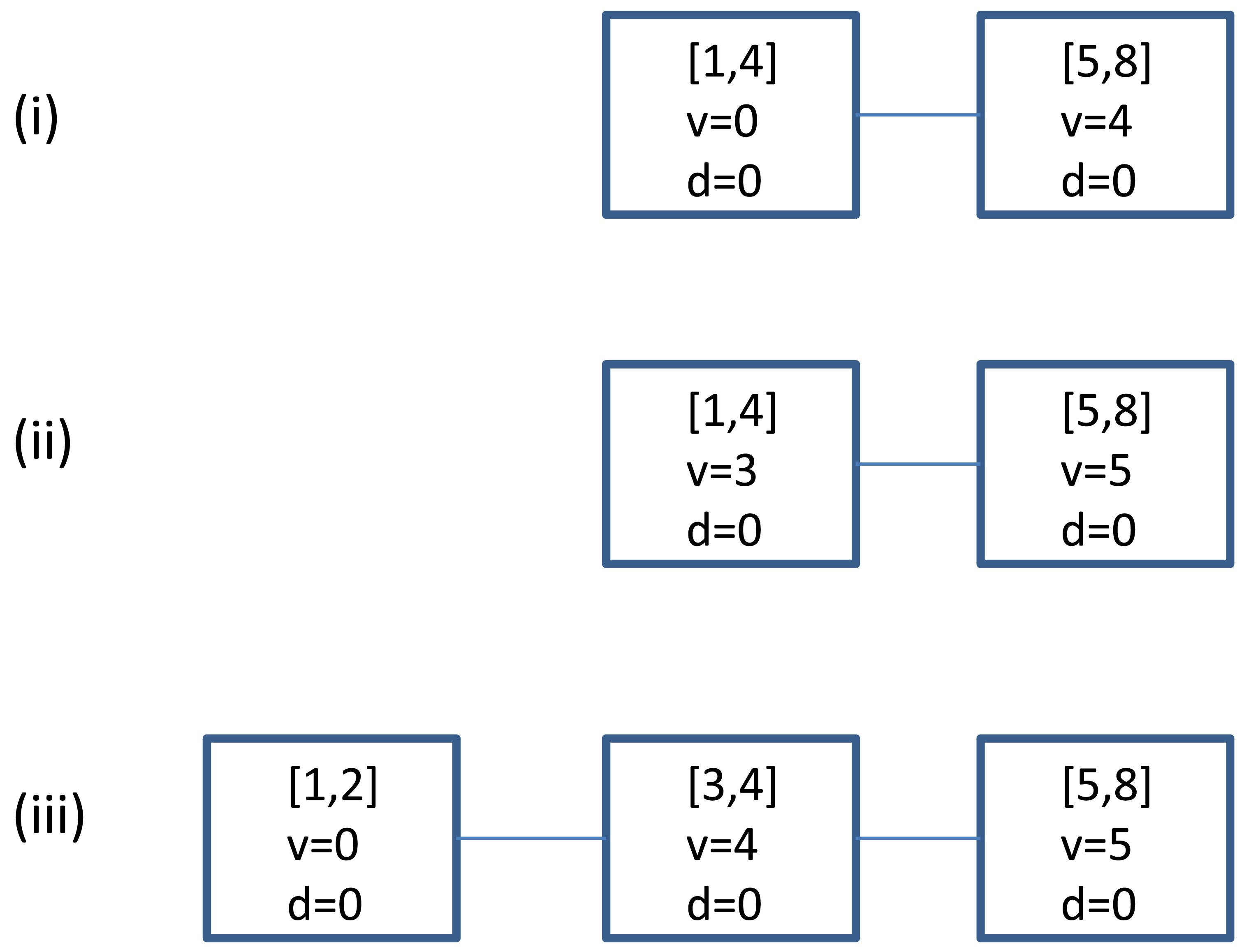
Figure 1 gives an example on how is updated using the procedure.
Obviously, a direct implementation of
I,λ,κ uses too much space. We now extend a technique of Misra and Gries [14] to reduce the space requirement. For any
, we say that
is trivial if the queue contains only a single node N with (i) i(N) = I, and (ii) v(N) = d(N) = 0. Every queue in
I,λ,κ is trivial initially. The key for reducing the space complexity of
I,λ,κ is to maintain the following invariant throughout the execution:
(*) There are at most κ non-trivial queues in
![Algorithms 04 00200i1]() I,λ,κ.
I,λ,κ.
We call κ the capacity of
I,λ,κ. The invariant helps us save space because we do not need to store trivial queues physically in memory. To maintain (*), each queue
supports the following procedure, which is called only when
, the total values of the nodes in
, is strictly greater than
, the total debits of the nodes in
.
| .Debit( ) | |
| 1: | if ( ) then |
| 2: | return error; |
| 3: | else |
| 4: | find an arbitrary node N of with v(N) > d(N); |
| 5: | /* such a node must exist because */ |
| 6: | d(N) = d(N) + 1; |
| 7: | end if |
Note from the implementation of Debit( ) that
is always no smaller than
, and for each node N of
. Furthermore, if
, then v(N) = d(N) for every node N in
. To maintain (*),
I,λ,κ processes a newly arrived item (a, u) with u ∈ I as follows.
| I,λ,κ.Process((a, u)) | |
| 1: | update by calling .Update((a, u)); |
| 2: | if (after the update the number of non-trivial queues becomes κ) then |
| 3: | for each with do.Debit( ); |
| 4: | for each non-trivial queues with do |
| 5: | delete all nodes of and make it a trivial queue; |
| 6: | /* Note that each deleted node N satisfies v(N) = d(N). */ |
| 7: | end if |
It is easy to see that Invariant (*) always holds: Initially the number m of non-trivial queues is zero, and m increases only when Process((a, u)) is on some trivial ; in such case becomes 1 and remains 0. If m becomes κ after this increase, we will debit, among other queues, and its becomes 1 too. It follows that , and Lines 4–5 will make trivial and m becomes less than κ again.
We are now ready to define
I,λ,κ's estimate f̂a([t, rI]) of fa([t, rI]) and analyze its accuracy. We need some definitions. For any interval J = [p, q] and any t ∈ I, we say that J covers t if t ∈ [p, q], is to the right of t if t < p, and is to the left of t otherwise. For any item a and any t ∈ I = [ℓI, rI],
I,λ,κ's estimate of fa([t, rI]) is
f̂a([t, rI]) = the value sum of the nodes N currently in whose i(N) covers or is to the right of t.
For example, in Figure 1, after the update of the last item (a, 1), we can obtain the estimate f̂a([2, 8]) = 0 + 4 + 5 = 9.
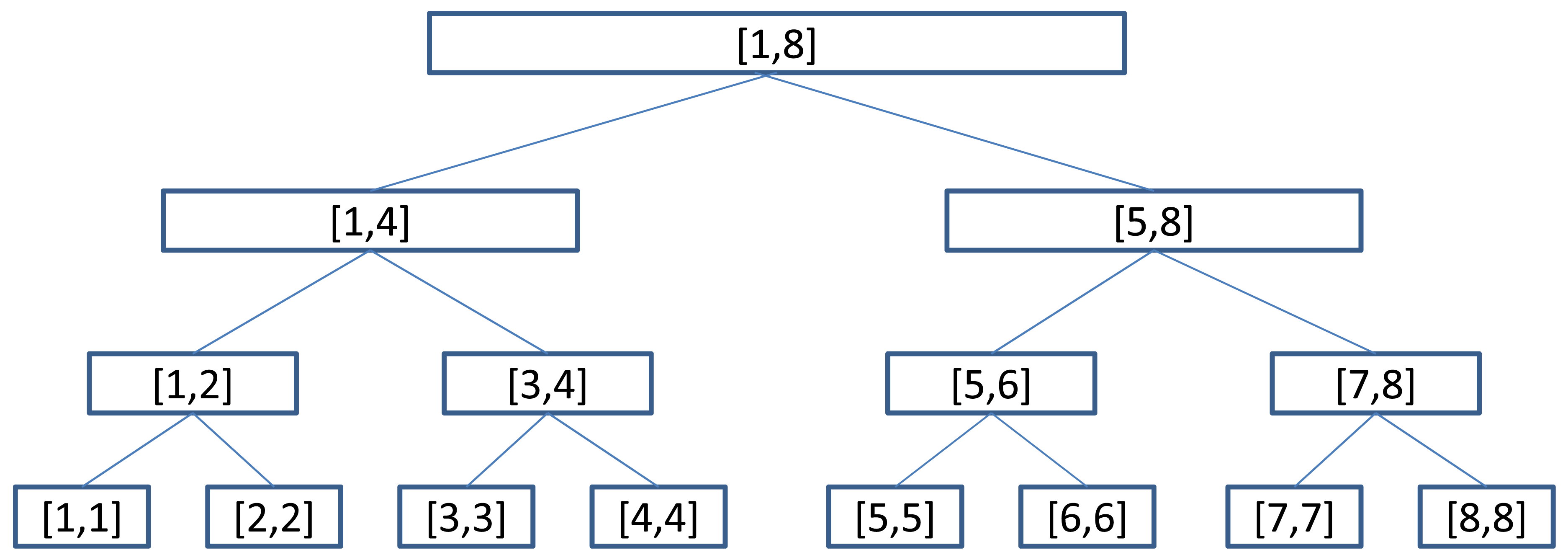
Given any node N of , we say that N is monitoring a over J, or simply N is monitoring J if i(N) = J. Note that a node may monitor different intervals during different periods of execution, and the size of these intervals are monotonically decreasing. Observe that although there are about W2/2 possible sub-intervals of size-W interval I, there are only about 2W of them that would be monitored by some nodes: there is only one such interval of size W, namely I = [ℓI, rI], which gives birth to two such intervals of size W/2, namely [ℓI, m] and [m + 1, rI] where m = ⌊(ℓI + rI)/2⌋, and so on. We call these O(W) intervals interesting intervals. For any two interesting intervals J and H such that J ⊂ H, we say that J is a descendant of H, and H is an ancestor of J. Figure 2 shows all the interesting intervals for I = [1, 8], as well as their ancestor-descendant relationship. The following important fact is easy to verify by induction.
Fact 1
Any two interesting intervals J and H do not cross, although one can contain another, i.e., either J ⊂ H, or H ⊂ J, or J ∩ H = ∅. Furthermore, any interesting interval has at most logW ancestors.
For any node N, let
 (N) be the set of intervals that have been monitored by N so far. The following fact can be verified from the update procedure.
Fact 2
Consider a node N in , where i(N) = J.
If J covers or is to the right of t, then all intervals in
![Algorithms 04 00200i4]() (N) cover or are to the right of t.
(N) cover or are to the right of t.If J is to the left of t, then all intervals in
![Algorithms 04 00200i4]() (N) are to the left of t.
(N) are to the left of t.
We say that N covers or is to the right of t if the intervals in
(N) cover or are to the right of t; otherwise, N is to the left of t. For any queue
, let alive
be the set of nodes currently in
, dead
be those nodes of
that have already been deleted (because of Line 5 of the procedure Process( )), and node
. Note that the estimate f̂a([t, ri]) is the value sum of the nodes in alive
that cover or are to the right of t. For simplicity, we need to express it more succinctly. Let
I,λ,κ. Define dead(
I,λ,κ) and node(
I,λ,κ) similarly. For any item a and any subset X ⊆ node(
I,λ,κ), let Xa be the set of nodes in X that are monitoring a (and thus are the nodes from
). For any t ∈ I, let X≥t denote the set of nodes in X that cover or are to the right of t. Define v(X) = ΣN∈X v(N) and d(X) = ΣN∈X d(N). Then, f̂a([t, rI]) can be expressed as follows:
The following theorem analyzes its accuracy, as well as gives the size of
I,λ,κ.
Lemma 3
For any t ∈ I, fa([t, rI]) −
f*(I) ≤ f̂a([t, rI]) ≤ fa([t, rI]) + λ logW. Furthermore,
I,λ,κ has size O(f*(I)/λ + κ) words.
Proof
Recall that
. Consider any node N ∈ alive
. Note that v(N) = ΣJ∈
 (N) vadd(N, J) where vadd(N, J) is the value added to v(N) during the period when i(N) = J. By Fact 2, we can divide it as v(N) = Σ{vadd(N, J) | J covers t} + Σ {vadd(N, J) | J is to the right of t}. It follows that
Note that , because if an arrived item (a, u) causes an increase of vadd(N, J) for some J that is to the right of t, then u must be in [t, rI]. By Equation (5), to show the second inequality of the lemma, it suffices to show that is no greater than λ logW, as follows.
Without loss of generality, suppose |J1| ≥ |J2| ≥ ⋯≥ |Jκ|. It can be verified that once an interval J is assigned to a node, it will not be assigned to other nodes; thus the Ji's are distinct. Furthermore, note that for 1 ≤ i < k, Jκ ⊂ Ji because (i) t is in both Ji and Jκ; (ii) Jκ is the smallest interval; and (iii) interesting intervals do not cross; thus Jκ is a descendant of Ji, and together with Fact 1, k ≤ logW. By Line 3 of the procedure Update( ), vadd(Ni, Ji) ≤ λ for 1 ≤ i ≤ k. It follows that So ≤ λ logW.
For the first inequality of the lemma, it is clearer to use . Note that every arrived item (a, u) with u ∈ [t, rI] increments the value of some node in node ; thus and
From Lines 4–6 of the procedure Process( ), when we delete a node N, v(N) = d(N). Hence, , which is equal to the total number of debit operations made to these dead nodes. Since whenever we make a debit operation to , we will make a debit operation to κ − 1 other queues,
In summary, we have , and the first inequality of the lemma follows.
For the space, we say that a node is born-rich if it is created because of Line 5 of the procedure Update( ) (and thus has λ items under its belt); otherwise it is born-poor. Obviously, there are at most f*(I)/λ born-rich nodes. For born-poor nodes, we need to store at most κ of them because every queue has one born-poor node (the rightmost one), and we only need to store at most κ non-trivial queues; the space bound follows.
If we set λ = λi = ∊2i/logW and , then Lemma 3 asserts that is an -space data structure that enables us to obtain, for any item a ∈ U and any timestamp t ∈ I, an estimate f̂a([t, rI]) that satisfies
If f*(I) does not vary too much, we can determine the i such that f* (I) ≈ 2i, and is an space data structure that guarantees an error bound of O(∊f*(I)). However, this approach has two obvious shortcomings:
f*(I) may vary from some small value to a value as large as B, the maximum number of items falling in a window of size W; hence, there may not be any fixed i that always satisfies f* (I) ≈ 2i
To estimate fa([t, rI]), we need an error bound of ∊f*([t, rI]), not ∊f*(I).
We will explain how to overcome these two shortcomings in the next section.
4. Our Data Structure for ∊-approximate Counting
The first shortcoming of the approach given in Section 3 is easy to overcome: a natural idea is to maintain
for different λi to handle different possible values of f*(I). The second shortcoming is more fundamental. To overcome it, we need to modify
I,λ,κ substantially The result is a new and complicated data structure
, where Y is an integer determining the accuracy As asserted in Theorem 7 below, this data structure uses
space, supports
update time, and for any t ∈ I, it offers the following special guarantee:
When can return, for any item a, an estimate f̂a([t, rI]) of fa([t, rI]) such that |f̂a([t, rI])−fa([t, rI])|≤∊Y.
When does not have any error bound on its estimate f̂a([t, rI]).
Before giving the details of
, let us explain how to use it to build the data structure
I,∊ mentioned in Section 2 for the ∊-approximate counting problem. To build
I,∊, we need another
-space data structure
I,∊, which is a simple adaption of the data structure
∊ of Cormode et al. [1] for the ∊-approximate basic counting problem;
I,∊ enables us to find, for any t ∈ I, an estimate f̂*([t, rI]) of f*([t, rI]) such that
I,∊ is implemented as follows. During execution, we maintain the data structure
∊/4 of Cormode et al. to count the items in the sliding window. When τcur = rI, we duplicate
∊/4 and get
′. Then,
′ is updated as if τcur was fixed at rI. To get the estimate f̂*([t, rI]), we first obtain an estimate f′ of f*([t, rI]) from
′, which satisfies
. Then,
. It can be verified that f̂*([t, rI]) satisfies Equation (7). Our data structure
I,∊ is composed of (i)
I,∊, and (ii)
for each integer i from
. It also maintains a brute-force
-space data structure for remembering the
items (a, u) with the largest u ∈ I; this brute-force data structure will be used for finding f̂a([t, rI]) only when
.
Theorem 4
The data structure
![Algorithms 04 00200i2]() I,∊ has size
words, and supports
update time.
I,∊ has size
words, and supports
update time.Given
![Algorithms 04 00200i2]() I,∊, we can find, for any a ∈ Σ and t ∈ I, an estimate of f̂a([t, rI]) of fa([t, rI]) such that |f̂a([t, rI]) − fa([t, rI])| ≤ ∊f*([t, rI]).
I,∊, we can find, for any a ∈ Σ and t ∈ I, an estimate of f̂a([t, rI]) of fa([t, rI]) such that |f̂a([t, rI]) − fa([t, rI])| ≤ ∊f*([t, rI]).
Proof
Statement (i) is straightforward because there are different , each has size and takes time for an update. For Statement (ii), we describe how to get the estimate and analyze its accuracy.
First, we use
I,∊ to get the estimate f̂*([t, rI]). If
, then
and we can use the brute-force data structure to find fa([t, rI]) exactly. Otherwise, we determine the i with 2i−1 < f̂*([t, rI]) ≤ 2i. Note that
and we have the data structure , and
f*([t, rI]) ≤ f̂*([t, rI]) ≤ 2i.
We use to obtain an estimate f̂a([t, rI]) with . By Equation (7), 2i−1 < f̂*([t, rI]) ≤ (1 + ∊)f*([t, rI]). Combining the two inequalities we have
We now describe the construction of . First, we describe an -space version of the data structure. Then, we show in the next section how to reduce the space to . In our discussion, we fix λ = ∊Y/logW and .
Initially,
is just the data structure
I,λ,κ. By Lemma 3, we know that its size is
, which is
when f*(I) ≤ Y. However, it is much larger than
when f*(I) ≫ Y, and to maintain small space usage in such case, we trim
I,λ,κ by throwing away a significant number of nodes. This is acceptable because
I,λ,κ only guarantees good estimates for those t ∈ I with f*([t, rI]) ≤ Y. The trimming process is rather tricky. The natural idea of throwing away all the nodes to the left of t when we find f*([t, rI]) > Y does not work because the resulting data structure may return estimates with error larger than the required ∊Y bound. For example, let I = [1, W]. For each item ai ∈ {a1, a2, …, aκ−1}, there are m = Y/κ copies of (ai, t + 1) arrive at time W + t for every t ∈ [0, W − 1]. Also, there are m copies of (a, W) arrive at time W + t for every t ∈ [0, W − 1]. Hence, at each time W + t, there are mκ = Y items with timestamps in [t, W] arrives, m items for each of the κ item name in {a, a1, …, aκ−1}. We are interested in the accuracy of the estimate f̂a([W, W]). It can be verified that at each time W + t, Lines 4–5 of the procedure Process( ) will eventually trivialize
and thus f̂a([W, W]) = 0. Since fa([W, W]) = (t + 1)m, |f̂a([W, W]) − fa([W, W])| = (t + 1)m. When t = 2∊Y/m − 1, the absolute error is 2∊Y which is larger than the required error bound ∊Y.
To describe the right trimming procedure, we need some basic operations. Consider any
J,λ,κ where J = [p, q]. The following operation splits
J,λ,κ into two smaller data structures
Jℓ,λ,κ and
Jr,λ,κ where Jt = [p, m] and Jr = [m+ 1, q] with m = ⌊(p + q)/2⌋.
| .Split(
J,λ,κ) | |
| 1: | for each non-trivial queue do |
| 2: | if ( has only one node N monitoring the whole interval J) then |
| 3: | /* refine J */ |
| 4: | insert a new node N′ immediately to the left of N with v(N′) = d(N′) = 0; |
| 5: | i(N′) = Jℓ, and i(N) = Jr; |
| 6: | end if |
| 7: | divide into two sub-queues and where |
| 8: | contains the nodes monitoring some sub-intervals of Jℓ, and |
| 9: | contains those monitoring some sub-intervals of Jr; |
| 10: | put
in
Jℓ,λ,κ and
in
Jr,λ,κ. |
| 11: | end for |
| 12: | /* For a trivial
, its two children in
Jℓ,λ,κ and
Jr,λ,κ are also trivial. */ |
We say that
Jℓ,λ,κ and
Jr,λ,κ are the left and right child of
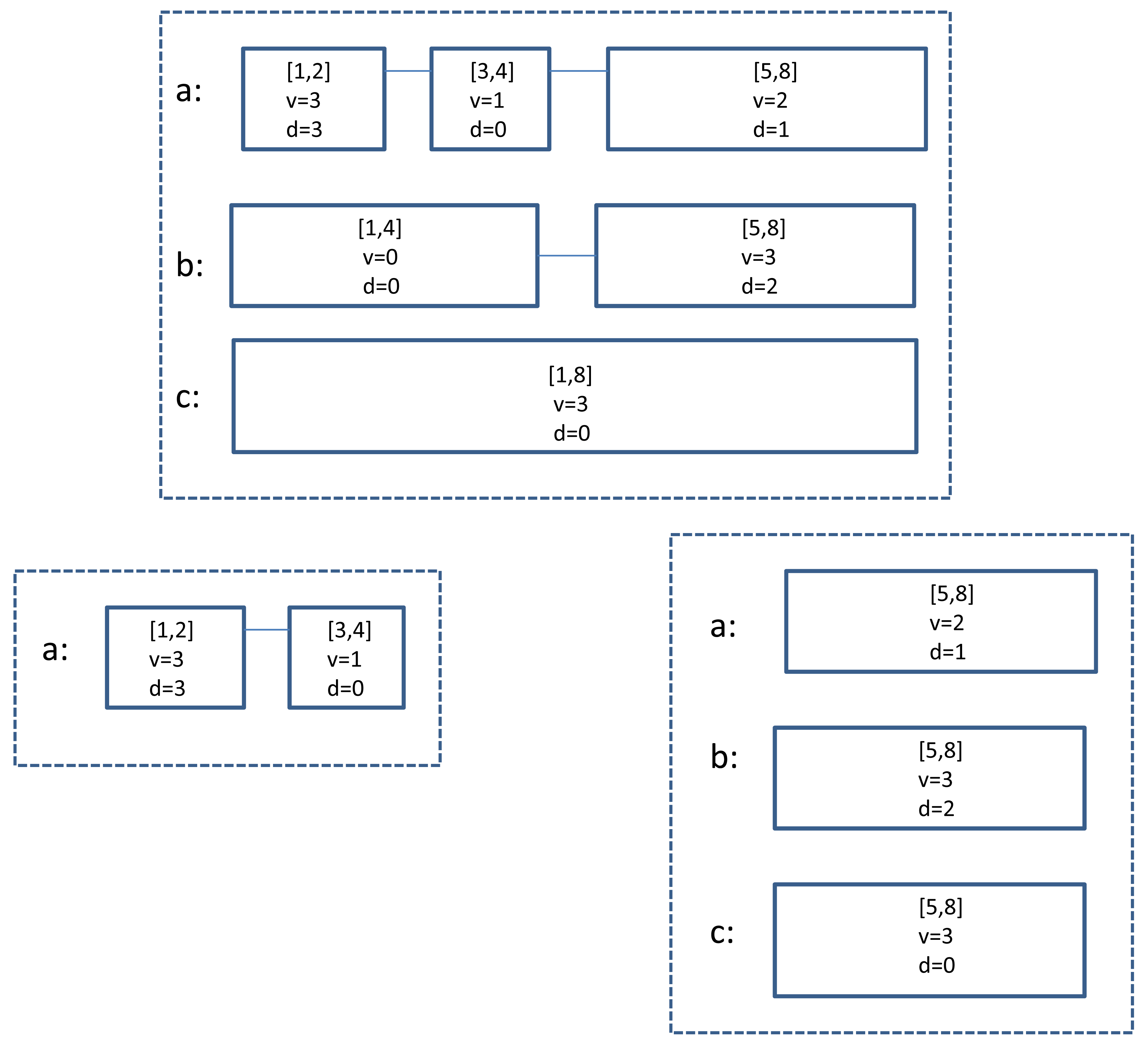
Jr,λ,κ, respectively. Figure 3 gives an example of Split(
[1,8],λ,κ), the split of
[1,8],λ,κ, which has three non-trivial queues
,
and
, into
[1, 4],λ,κ and
[5, 8],λ,κ. Note that the queues for b and c in
[1, 4],λ,κ are trivial and we have not stored them.
Using Split( ), we can trim, for example,
[p,p+1],λ,κ into
[p+1,p+1],λ,κ as follows: Split
[p,p+1],λ,κ into
[p,p],λ,κ and
[p+1,p+1],λ,κ, and throw away
[p, p],λ,κ. The following recursive procedure LeftRefine( ) generalizes this idea for larger J: Given
J,λ,κ =
[p, q],λ,κ, it returns a list 〈
J0,λ,κ,
J1,λ,κ, …,
Jm,λ,κ〉 where the Ji's form a partition of [p, q], and J0 = [p, p]. Throwing away
J0,λ,κ, and the remaining
Ji,λ,κ's all together monitor [p + 1, q].
| .LeftRefine (
[p,q],λ,κ) | |
| 1: | if (|[p, q]| = |[p, p]| = 1) then |
| 2: | return 〈
[p,p],λ,κ〉; |
| 3: | else |
| 4: | split
[p,q],λ,κ into its left child
[p, m],λ,κ and right child
[m+1,q],λ,κ |
| 5: | /* where m = ⌊(p + q)/2⌋ */; |
| 6: | L = LeftRefine(
[p, m],λ,κ); |
| 7: | suppose L = 〈
J0,λ,κ,
J1,λ,κ, …,
Jk,λ,κ〉; |
| 8: | return 〈
J0,λ,κ, …,
Jk,λ,κ [m+1,q],λ,κ〉; |
| 9: | end if |
For example, LeftRefine(
[1,8],λ,κ) gives us the list 〈
[1,1],λ,κ,
[2, 2],λ,κ,
[3, 4],λ,κ,
[5,8],λ,κ〉. Note that J0 = [p, p] because the recursion stops only when |[p, q]| = 1. The list returned by LeftRefine(
[p, q],λ,κ) has another useful property, which we describe below.
Given L = 〈
Z1,λ,κ, …,
Zk,λ,κ), we say that L is an interesting-partition covering the interval J if (i) the Zi's are all interesting intervals and form a partition of J; and (ii) for 1 ≤ i < k, Zi is to the left of Zi+1, and
. The fact below can be verified by induction on the length of the list returned by LeftRefine( ).
Fact 3
Let J be an interesting interval, and L = 〈
J0,λ,κ, …,
Jm,λ,κ〉 be the list returned by LeftRefine(
J,λ,κ). Then, the list 〈
J1,λ,κ, …,
Jm,λ,κ 〉 (i.e., the list obtained by throwing away the head
J0,λ,κ of L) is an interesting-partition covering [p + 1, q].
For example, if [1, 8] is an interesting interval, then the list 〈
[2,2],λ,κ [3,4],λ,κ [5,8],λ,κ〉 obtained by throwing away the first element
[1,1],λ,κ from LeftRefine(
[1,8],λ,κ) is an interesting-partition covering [2, 8].
We now give details of . Initially, it is the interesting-partition 〈CI,λ,κ 〉 covering the whole interval I = [ℓI, rI]. Throughout the execution, we maintain the following invariant:
(**) is an interesting-partition covering some [p, rI] ⊆ I.
When is covering [p, rI], it only guarantees good estimates of fa([t, rI]) for t ∈ [p, rI], and this estimate is obtained by
Ji,λ,κ in
where u ∈ Ji, update it by calling
Ji,λ,κ. Process((a, u)). Note that this update has no effect on the other
J,λ,κ in
.During execution, we also keep track of the largest timestamp pmax ∈ I such that the estimate f̂*(pmax,rI]) given by
I,∊ is greater than (1 + ∊)Y (which implies f*([pmax,rI]) > Y because of Equation (7)). As soon as pmax falls in the interval covered by
, we use the following procedure to trim
to cover the smaller interval [pmax + 1, rI].
Suppose that L = 〈
J1,λ,κ, …,
Ji,λ,κ) is an interesting-partition covering [p, rI], and t ∈ [p, rI]. Trim(L, t) constructs an interesting-partition covering [t + 1, rI] recursively as follows.
| .Trim(L, t) | |
| 1: | find the unique
Ji,λ,κ in L such that t ∈ Ji; |
| 2: | L′ =LeftRefine(
Ji,λ,κ); |
| 3: | suppose L′ = 〈
K0,λ,κ, …,
K1,λ,κ,
Kℓ,λ,κ〉; |
| 4: | if (K0 = [t, t]) then |
| 5: | return 〈
K1,λ,κ, …,
Kℓ,λ,κ,
Ji+1,λ,κ,
Jm,λ,κ 〉; |
| 6: | /* i.e., throw away
J1,λ,κ, …,
Ji−1,λ,κ, and
K0,λ,κ, */ |
| 7: | /* and return an interesting-partition covering [t + 1, rI]. */ |
| 8: | else |
| 9: | return Trim(〈
K1,λ,κ, …,
Kℓ,λ,κ,
Ji+1,λ,κ,
Jm,λ,κ 〉, t). |
| 10: | /* throw away
J1,λ,κ, …,
Ji−1,λ,κ and
K0,λ,κ */ |
| 11: | end if |
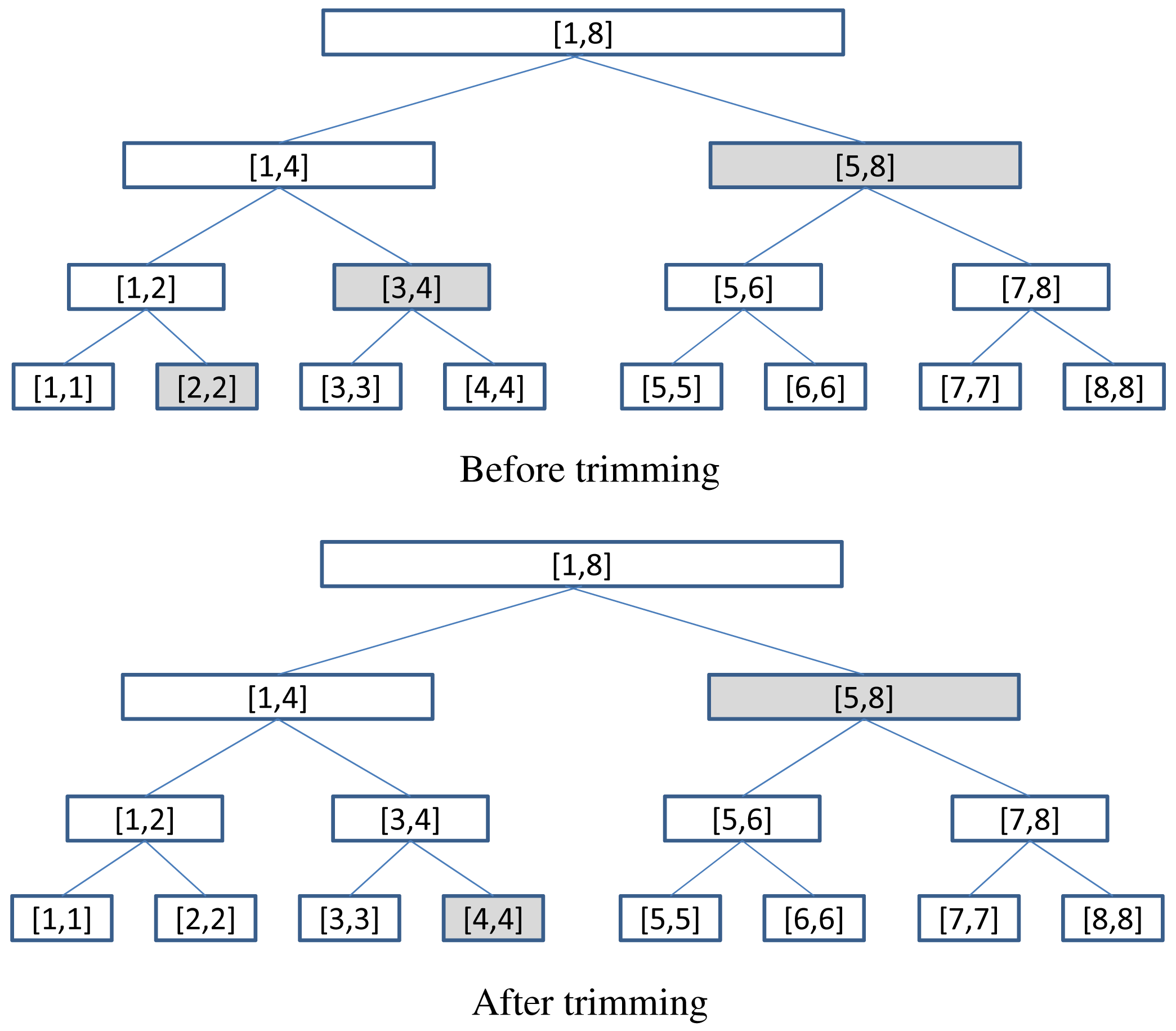
For example, Figure 4 shows that when
,
return 〈
[4,4],λ,κ,
[5,8],λ,κ 〉. Based on Fact 3, it can be verified inductively that after
, the new
is an interesting-partition covering [pmax + 1, rI]; Invariant (**) is preserved. In the rest of this section, we analyze the size of
and the accuracy of its estimates.
Let All be the set of all
J,λ,κ's that ever exist, i.e., if
J,λ,κ ∈ All, then either (i) it is currently in
, or (ii) it has been in
some time earlier in the execution, but is thrown away during some trimming of
. For any p ∈ I, define
Let vadd(
J,λ,κ) be the total value added to the nodes of
J,λ,κ during its lifespan. We now derive an upper bound on Σ  J,λ,κ ∈ All≥p vadd(
J,λ,κ), which is crucial for getting a tight error bound on the accuracy of
's estimates.
J,λ,κ ∈ All≥p vadd(
J,λ,κ), which is crucial for getting a tight error bound on the accuracy of
's estimates.
Recall that initially
and thus
I,λ,κ ∈ All. For any other
J,λ,κ ∈ All,
J,λ,κ must be a child of some
H,λ,κ ∈ All (i.e.,
J,λ,κ is obtained from Split(
H,λ,κ))- Given
J,λ,κ and
H,λ,κ, we say that
J,λ,κ is a descendant of
H,λ,κ, and
H,λ,κ is an ancestor of
J,λ,κ, if either (i)
J,λ,κ is a child of
H,λ,κ, or (ii) it is a child of some of
H,λ,κ's descendants. Note that the original
I,λ,κ is an ancestor of every
J,λ,κ ∈ All, and in general, any
H,λ,κ ∈ All is an ancestor of every
J,λ,κ ∈ All with J ⊂ H. We have the following lemma. (Note that we are abusing the notation here and regard
as a set.)
Lemma 5
Suppose that is covering [p, rI]. Let be the set . Then,
,
vadd(
![Algorithms 04 00200i1]() J,λ,κ) ≤ (1 + ∊)Y for any
J,λ,κ) ≤ (1 + ∊)Y for any
![Algorithms 04 00200i1]() J,λ,κ ∈ All, and
J,λ,κ ∈ All, and.
Therefore, Σ{vadd(
J,λ,κ) |
J,λ,κ ∈ All≥p} ≤ 2(1 + ∊)Y logW.
Proof
For (1), it suffices to prove that for any
. By definition, J covers or is to the right of p; thus J ∩ (J1 ∪ ⋯ ∪ Jm) = J ∩ [p, rI] ≠ ∅. Since the intervals are interesting and do not cross, there is an 1 ≤ i ≤ m such that either (i) J = Ji, and thus
, or (ii) Ji ⊂ J, which implies
J,λ,κ is an ancestor of
J,λ,κ, i.e.,
. (It is not possible that J ⊂ Ji, otherwise
Ji,λ,κ would have been split and should not be in the current
. Hence,
.
To prove (2), suppose that J = [x, y] and vadd(
J,λ,κ) has just reached (1 + ∊)Y. This implies f*([x, rI]) ≥ (1 + ∊)Y, and so does its estimate f̂*([x, rI]) given by
I,∊ (as f*([x, rI]) ≤ f̂*([x, rI]), by Equation (7)). Then, the procedure Trim( ) will be called and
J,λ,κ will be either thrown away or split, and no more value can be added to
J,λ,κ. It follows that vadd(
J,λ,κ) ≤ (1 + ∊)Y.
For (3), recall that
. Among the intervals J1, …, Jm, interval J1 is the leftmost interval and its left boundary ℓJ1 = p. We now prove that
where anc(
J1,λ,κ) is the set of ancestors of
J1,λ,κ. Then, together with the facts that
(by Property (ii) of interesting-partition) and |anc(
J1,λ,κ)| ≤ logW (as each Split operation would reduce the size of interval by half), we have
To show
, it suffices to show that for any
,
H,λ,κ ∈ anc(
J1,λ,κ). Since
, it is the ancestor of some
. Thus Ji = [ℓji, rji] ⊂ H = [ℓH, rH]. Since
H,λ,κ is already an ancestor, it no longer exists, and all the
J,λ,κ to its left have been thrown away. Thus,
has no
J,λ,κ where J is to the right of ℓH. This implies ℓH ≤ p = ℓJ1 and ℓH ≤ ℓJ1 ≤ rJ1 ≤ rJi ≤ rH. It follows that J1 ⊂ H and
H,λ,κ is an ancestor of
J1,λ,κ, i.e.,
H,λ,κ ∈ anc(
J1,λ,κ).
We are now ready to analyze the accuracy of 's estimates.
Theorem 6
Suppose that is covering [p, rI]. For any item a and any t ∈ [p, rI], the estimate f̂a([t, rI]) of fa([t, rI]) obtained by satisfies |f̂a([t, rI]) − fa([t, rI])| ≤ ∊Y. Furthermore, uses space.
Proof
Let alive be the set of nodes currently in the set of those that were in earlier in the execution but have been deleted, and . It can be verified that . Below, we prove that
Recall that we fix λ = ∊Y/logW and ; the ∊Y error bound follows.
The proof of the second inequality of Equation (8) is identical to that of Lemma 3, except that we replace all occurrences of
J,λ,κ by
. The proof of the first inequality is also similar. We still have
Observe that for any node
, N can only be in those
J,λ,κ ∈ All≥p (because t ∈ [p, rI]), and when we debit N, if it is in
J,λ,κ, then we debit κ − 1 other nodes in
J,λ,κ monitoring κ − 1 items other than a. Thus,
is no more than the total value available in the
J,λ,κ ∈ All≥p, which is Σ {vadd(
J,λ,κ) |
J,λ,κ ∈ All≥p}. Together with Lemma 5 we conclude
For the size of
, similar to the proof of Lemma 3, we can argue that the number of born-rich nodes is only
, but the number of born-poor nodes can be much larger. A born-poor node of a non-trivial queue is created either when we increase the value of a trivial queue, or when we execute Lines 2-6 of procedure Split. It can be verified that every queue
has at most one born-poor node, which is the rightmost node in
. Since there are O(logW)
J,λ,κ's in
and each has at most κ non-trivial queues, the number of born-poor nodes, and hence the size of
, is
.
To reduce 's size from to , we need to reduce the number of born-poor nodes; or equivalently, the number of non-trivial queues in . In the next section, we give a simple idea to reduce the number of non-trivial queues and hence the size of to . In Section 6, we show how to further reduce the size by taking advantage of the tardiness of the data stream.
5. Reducing the Size of
Our idea for reducing the size is simple; for every
, its capacity is no longer fixed at
; instead, we start with a much smaller capacity, namely
, which is allowed to increase gradually during execution. To determine
J,λ,κ's capacity, we use a variable to keep track of the number f̄*(J) of items (a, u) with u ∈ J that have arrived since
J,λ,κ's creation. Let vJ be the total value of the nodes in
J,λ,κ when it is created (vJ may not be zero if
J,λ,κ is resulted from the splitting of its parent). The capacity of
J,λ,κ is determined as follows.
When for some integer c ≥ 1, the capacity of
![Algorithms 04 00200i1]() J,λ,κ is
, i.e., set κ = κ(c) and allow κ(c) non-trivial queues in
J,λ,κ is
, i.e., set κ = κ(c) and allow κ(c) non-trivial queues in
![Algorithms 04 00200i1]() J,λ,κ.
J,λ,κ.
Note that when we increase the capacity of
J,λ,κ to κ(c), we do not need to do anything, except that we allow more non-trivial queues (up to κ(c)) in the data structure. Also note that when
J,λ,κ is created during the trimming process, its inherited capacity may be larger than the supposed capacity κ(c); in such case, we simply debit every non-trivial queue until some queue
has
and we execute Lines 4 and 5 of the procedure Process( ) to make this queue trivial. We repeat the process until the number of non-trivial queues is at most κ(c). The following theorem asserts that
maintains the accuracy of its estimates under this new implementation. It gives the revised size and the update time.
Theorem 7
Suppose that is currently covering [p, rI]. For any item a ∈ Σ and any timestamp t ∈ [p, rI], the estimate f̂a([t, rI]) of f̂a([t, rI]) obtained by the new satisfies |f̂a([t, rI]) − fa([t, rI])| ≤ ∊Y.
has size , and supports update time.
Proof
Suppose that
. From the fact that we are using
Ji,λ,κ(ci) to monitor Ji we conclude
. It follows that
, which is O(Y) because (i)
and (ii)
(otherwise
would have been trimmed). Thus,
For Statement (1), the analysis of the accuracy of f̂a([t, rI]) is very similar to that of Theorem 6, except for the following difference: In the proof of Theorem 6, we show that , and since κ is fixed at , . Here, we also prove that , but we have to prove it differently because the capacities are no longer fixed.
As argued previously, any node in
is in some
J,λ,κ ∈ All≥p. Below, we show that for any
J,λ,κ ∈ All≥p, we can make at most
debit operations to the queue
of
J,λ,κ during its lifespan. Together with the fact that |All≥p| ≤ 2 logW, we have
.
Consider any
J,λ,κ ∈ All≥p. Note that the smaller its capacity, the larger the number of debit operations can be made to the queue
of
J,λ,κ. To maximize the number of debit operations made to
, suppose that vJ = 0 and thus
J,λ,κ has the smallest capacity κ(1) when it is created. Before increasing its capacity to κ(2),
J,λ,κ can make at most
debit operations to
. Then, during the next
arrivals of items (a, u) with
, the capacity is κ(2), and at most
debit operations can be made to
. In general, during the period when
, at most
debit operations can be made to
. If the largest capacity is κ(cmax), the total number of debit operations made to
is at most
We now prove (2). Note that the total number of non-trivial queues in , and hence the number of born-poor nodes, is at most . By Equation (9), , and it follows that the size of is .
For the update time, suppose that an item (a, u) arrives. We can find the
Ji,λ,κ in
with u ∈ Ji using O(log m) = O(log logW) time by querying a balanced search tree storing the Ji's. By hashing (e.g., Cuckoo hashing [15], which supports constant update and query time) we can locate the queue
in constant time. Then, by consulting an auxiliary balanced search tree on the intervals monitored by the nodes of
, we can find and update the node N of
with u ∈ i(N) using
time. At times we may also need to execute Lines 3 and 4 of the procedure Process( ), which debits all the non-trivial queues in
Ji,λ,κ. Using the de-amortizing technique given in [16], this step takes constant time.
Note that occasionally, we may also need to clean up by calling Trim( ); this step takes time linear to the size of , which is .
6. Further Reducing the Size of for Streams with Small Tardiness
Recall that in an out-of-order data stream with tardiness dmax ∈ [0, W], any item (a, u) arriving at time τcur satisfies u ≥ τcur − dmax; in other words, the delay of any item is guaranteed to be at most dmax. This section extends to a data structure that takes advantage of this maximum delay guarantee to reduce the space usage. The idea is as follows. Since there is no new item with stamps smaller than τCur − dmax, we will not make any further change to those nodes to the of left τcur − dmax and hence can consolidate these nodes to reduce space substantially. To handle those nodes with timestamps in [τcur − dmax, τcur], we use the data structure given in Section 5; since it is monitoring an interval of dmax instead of W, its size is instead of .
To implement , we need a new operation called consolidate. Consider any list of queues , where J1, J2, …, Jm are ordered from left to right and form a partition of the interval J1‥m = J1 ∪ ⋯ ∪ Jm. We consolidate them into a single queue as follows:
Concatenate the queues into a single queue, in which the nodes preserve the left-right order.
Starting from the leftmost node, check from left to right every node N in the queue, if N is not the rightmost node and v(N) < λ, merge it with the node N′ immediately to its right, i.e., delete N, set v(N′) = v(N) + v(N′), d(N′) = d(N) + d(N′) and
![Algorithms 04 00200i4]() (N′) =
(N′) =
![Algorithms 04 00200i4]() (N) ∪
(N) ∪
![Algorithms 04 00200i4]() (N′).
(N′).
Note that after the consolidation, the resulting queue has at most one node (the rightmost one) with value smaller than λ.
Given the list 〈
J1,λ,κ(c1), …,
Jm,λ,κ(cm)〉, we consolidate them into
by first consolidating, for each item a, the queues
in
J1,λ,κ(c1), …,
Jm,λ,κ(cm) into the queue
and put it in
. Then, we apply Lines 3–5 of procedure Process( ) repeatedly to reduce the number of non-trivial queues in the data structure to
.
We are now ready to describe how to extend to . In our discussion, we fix , and without loss of generality, we assume that I = [1, W]. Recall that pmax denotes the largest timestamp in I such that f̂*([pmax, rI]) > (1 + ∊)Y (which implies f*([pmax, rI]) > Y). We partition I into sub-windows I1, I2, …, Im, each of size dmax (i.e., Ii = [(i − 1)dmax, idmax]). We divide the execution into different periods according to τcur, the current time.
During the 1st period, when τcur ∈ [1, dmax] = I1, simply is .
During the 2nd period, when τcur = I2, maintains in addition to .
During the 3rd period, when τcur ∈ I3, maintains in addition to . Also, the is consolidated into .
In general, during the ith period, when maintains and , and also where I1‥i−2 = I1 ∪ I2 ∪ ⋯ ∪ Ii−2. Observe that in this period, there is no item (a, u) with u ∈ I1‥i−2 arrives (because the tardiness is dmax), and thus we do not need to update . However, we will keep throwing away any node N in as soon as we know i(N) is to the left of pmax + 1.
When entering the (i + 1)st period, we do the followings: Keep , create , merge
![Algorithms 04 00200i1]() I1‥i−2,λ,κ with
, and then get
by consolidating
.
I1‥i−2,λ,κ with
, and then get
by consolidating
.
Given any t ∈ [pmax + 1, rI], the estimate of fa([t, rI]) given by is
The following theorem gives the accuracy of 's size and its update time.
Theorem 8
For any t ∈ [pmax + 1, rI], the estimate f̂a([t, rI]) given by satisfies
has size , and supports update time.
Proof
Recall that I is partitioned into sub-intervals I1, I2, …, Im. Suppose that t ∈ Iκ. Note that if we had not performed any consolidation,
Note that for κ + 1 ≤ i ≤ m, , and for since |Iκ|= dmax, the same argument used in the proof of Lemma 3 gives us . Hence
The consolidation step may add errors to . To get a bound on them, let N1, N2, … be the nodes for a in , ordered from left to right. Suppose that t ∈ Nh. Note that
the consolidation step will added at most λ units to v(Nh) before we move on to consider the node immediately to its right, and
for node Ni with i ≥ h + 1, any node N that has been merged to Ni must be to the right of of Nh, and thus is to the right of t; it follows that N is contributing v(N) to in Equation (10) and its merging will not make any change.
In conclusion, the consolidation steps introduce at most λ extra errors, and Equation (10) becomes , which is the second inequality of the lemma.
To prove the first inequality, suppose that we ask for the estimate f̂a([t, rI]) during the ith period, when we have
,
and
. Recall that
I1‥i−2, λ,∊ comes from consolidating
. As in all our Previous analyses, we have
(Note that the merging of nodes during consolidations would not take away any value). To get a bound on , suppose that pmax ∈ Iκ. Then, all the nodes to the left of Iκ have been thrown away. Among , only may have been trimmed. Note that
,
as in the proof of Theorem 7, we can argue that , and
for the other , since their capacity is at least
Thus, , and the first inequality follows.
For Statement (2), note that both and have size (by Theorem 7, and |Ii−1| = |Ii| = dmax), and for , it has size ; thus the size of is . For the update time, it suffices to note that it is dominated by the update times of and .

 [1, 8], λ,κ.
 [2, 2],λ,κ,
[3, 4],λ,κ,
[5, 8],λ,κ〉, 3).
[2, 2],λ,κ,
[3, 4],λ,κ,
[5, 8],λ,κ〉, 3).

| Space Complexity (words) | |
|---|---|
| Synchronous [7] | |
| Asynchronous [1] | |
| Asynchronous [†] | |
| Asynchronous with tardiness [†] | |
Acknowledgments
H.F Ting is partially supported by the GRF Grant HKU-716307E; T.W. Lam is partially supported by the GRF Grant HKU-713909E.
References
- Cormode, G.; Korn, F.; Tirthapura, S. Time-Decaying Aggregates in Out-of-Order Streams. Proceedings of the 27th ACM SIGMOD-SIGACT-SIGART Symposium on Principles of Database Systems, PODS'08, Vancouver, Canada, 9–11 June 2008; pp. 89–98.
- Karp, R.; Shenker, S.; Papadimitriou, C. A simple algorithm for finding frequent elements in streams and bags. ACM Trans. Database Syst. 2003, 28, 51–55. [Google Scholar]
- Demaine, E.; Lopez-Ortiz, A.; Munro, J. Frequency Estimation of Internet Packet Streams with Limited Space. Proceedings of the 10th Annual European Symposium, ESA'07, Rome, Italy, 17–21 September 2002; pp. 348–360.
- Muthukrishnan, S. Data Streams: Algorithms and Applications; Now Publisher Inc.: Boston, MA, USA, 2005. [Google Scholar]
- Babcock, B.; Babu, S.; Datar, M.; Motwani, R.; Widom, J. Models and Issues in Data Stream Systems. Proceedings of the 21st ACM SIGACT-SIGMOD-SIGART Symposium on Principles of Database Systems, PODS'02, Madison, WI, USA, 3–5 June 2002; pp. 1–16.
- Arasu, A.; Manku, G. Approximate Counts and Quantiles over Sliding Windows. Proceedings of the 23th ACM SIGMOD-SIGACT-SIGART Symposium on Principles of Database Systems, PODS'04, Paris, France, 14–16 June 2004; pp. 286–296.
- Lee, L.K.; Ting, H.F. A Simpler and More Efficient Deterministic Scheme for Finding Frequent Items over Sliding Windows. Proceedings of the PODS, Chicago, Illinois, USA, June 26–28, 2006; pp. 290–297.
- Lee, L.K.; Ting, H.F. Maintaining Significant Stream Statistics over Sliding Windows. Proceedings of the 7th Annual ACM-SIAM Symposium on Discrete Algorithms, SODA'06, Miami, FL, USA, 22–26 January 2006; pp. 724–732.
- Datar, M.; Gionis, A.; Indyk, P.; Motwani, R. Maintaining stream statistics over sliding windows. SIAMJ. Comput. 2002, 31, 1794–1813. [Google Scholar]
- Tirthapura, S.; Xu, B.; Busch, C. Sketching Asynchronous Streams over a Sliding Window. Proceedings of the 25th Annual ACM SIGACT-SIGOPS Symposium on Principles of Distributed Computing, PODC'06, Denver, CO, USA, 23–26 July 2006; pp. 82–91.
- Busch, C.; Tirthapua, S. A Deterministic Algorithm for Summarizing Asynchronous Streams over a Sliding Window. Proceedings of the 24th Annual Symposium on Theoretical Aspects of Computer Science, STACS'07, Aachen, Germany, 22–24 February 2007; pp. 465–475.
- Cormode, G.; Tirthapura, S.; Xu, B. Time-decaying sketches for robust aggregation of sensor data. SIAM J. Comput. 2009, 39, 1309–1339. [Google Scholar]
- Chan, H.L.; Lam, T.W.; Lee, L.K.; Ting, H.F. Approximating Frequent Items in Asynchronous Data Stream over a Sliding Window. Proceedings of the 7th Workshop on Approximation and Online Algorithms, WAOA'09, Copenhagen, Denmark, 10–11 September 2009; pp. 49–61.
- Misra, J.; Gries, D. Finding repeated elements. Sci. Comput. Program. 1982, 2, 143–152. [Google Scholar]
- Arbitman, Y.; Naor, M.; Segev, G. De-amortized Cuckoo Hashing: Provable Worst-Case Performance and Experimental Results. Proceedings of the 36th International Colloquium, ICALP'09, Rhodes, Greece, 5–12 July 2009; pp. 107–118.
- Hung, R.S.; Lee, L.K.; Ting, H.F. Finding frequent items over sliding windows with constant update time. Inf. Process. Lett. 2010, 110, 257–260. [Google Scholar]
© 2011 by the authors; licensee MDPI, Basel, Switzerland. This article is an open access article distributed under the terms and conditions of the Creative Commons Attribution license (http://creativecommons.org/licenses/by/3.0/).
Share and Cite
Ting, H.-F.; Lee, L.-K.; Chan, H.-L.; Lam, T.-W. Approximating Frequent Items in Asynchronous Data Stream over a Sliding Window. Algorithms 2011, 4, 200-222. https://doi.org/10.3390/a4030200
Ting H-F, Lee L-K, Chan H-L, Lam T-W. Approximating Frequent Items in Asynchronous Data Stream over a Sliding Window. Algorithms. 2011; 4(3):200-222. https://doi.org/10.3390/a4030200
Chicago/Turabian StyleTing, Hing-Fung, Lap-Kei Lee, Ho-Leung Chan, and Tak-Wah Lam. 2011. "Approximating Frequent Items in Asynchronous Data Stream over a Sliding Window" Algorithms 4, no. 3: 200-222. https://doi.org/10.3390/a4030200
APA StyleTing, H.-F., Lee, L.-K., Chan, H.-L., & Lam, T.-W. (2011). Approximating Frequent Items in Asynchronous Data Stream over a Sliding Window. Algorithms, 4(3), 200-222. https://doi.org/10.3390/a4030200