Defense of the Least Squares Solution to Peelle’s Pertinent Puzzle

Abstract
: Generalized least squares (GLS) for model parameter estimation has a long and successful history dating to its development by Gauss in 1795. Alternatives can outperform GLS in some settings, and alternatives to GLS are sometimes sought when GLS exhibits curious behavior, such as in Peelle's Pertinent Puzzle (PPP). PPP was described in 1987 in the context of estimating fundamental parameters that arise in nuclear interaction experiments. In PPP, GLS estimates fell outside the range of the data, eliciting concerns that GLS was somehow flawed. These concerns have led to suggested alternatives to GLS estimators. This paper defends GLS in the PPP context, investigates when PPP can occur, illustrates when PPP can be beneficial for parameter estimation, reviews optimality properties of GLS estimators, and gives an example in which PPP does occur.1. Introduction
Generalized least squares (GLS) for parameter estimation has a long and successful history dating to its development by Gauss in 1795. In some settings, alternatives to GLS can be effective, and are sometimes sought when GLS exhibits curious behavior, such as in Peelle's Pertinent Puzzle (PPP).
PPP was introduced in 1987 in the context of estimating fundamental parameters that arise in nuclear interaction experiments [1]. PPP is described below and when it occurs, the GLS estimate of the parameter is guaranteed to be outside the range of the data, which has elicited concerns that GLS is flawed and has led to suggested alternatives to GLS estimators.
A GLS estimate lying outside the range of the data causes heartache among nuclear scientists. Therefore, PPP continues to be of theoretical and practical interest. For example, a summary report of International Evaluation of Neutron Cross Section Standards [2] discusses PPP in terms of a standard least-squares procedure. Neutron cross sections are fundamental parameters that describe the probabilities of various neutron interactions. These cross sections are typically estimated from multiple experiments so some type of weighted average estimation scheme is used. The cross section estimates from any two experiments can have shared errors arising for example from using the same measured background, which can lead to covariance structures such as those described below.
We quote the original PPP problem proposed by [1] from a report of Chiba and Smith [3], “Suppose we are required to obtain the weighted average of two experimental results for the same physical quantity. The first result is 1.5, and the second result 1.0. The full covariance matrix of those data is believed to be the sum of three components. The first component is fully correlated with standard error 20% of each respective value. The second and third components are independent of the first and of each other, and correspond to 10% random uncertainties in each experimental result.
Although this PPP statement is vague, by converting it to something more interpretable, GLS can be applied and the resulting estimate is 0.88 (with an associated standard deviation of 0.22), which is outside the range of the measurements. Zhao and Perey [4] re-interpreted PPP by introducing a third datum c, through which the common error can be explicitly specified as follows, “Suppose we have two independent measurements. One is m1 = 1.5 ± 10%. Another is m2 = 1.0 ± 10%. To convert this quantity into another physical quantity, we need a conversion factor c, which after intermediate steps omitted here is 1.0 with uncertainty of 20%. Now the experimental results are, y1 = cm1 = 1.5 and y2 = cm2 = 1.0. We are required to obtain the weighted average of those experimental data.
In this interpretation, the common error (the “fully correlated” component) is understood to be multiplicative, and m1 = 1.5 ± 10% is assumed to mean that the true standard deviation is 0.15 for m1 (and 0.10 for m2). Even after these interpretations, some vagueness remains. There is no convention regarding what confidence is associated with ±10%. Nor is there a convention for whether the standard deviation includes all error sources, or only includes random error effects, ignoring accuracy. In addition, we show below that it can matter whether the standard deviation is expressed as a fraction of the true quantity or of the measured quantity.
One of our contributions is to make explicit assumptions and examine their implications in order to convert vague statements to statements about which it is possible to find agreement among physical scientists and statisticians regarding suitable approaches. We also defend GLS in the PPP context, illustrate when PPP can be beneficial, briefly describe properties of GLS estimators, show that PPP cannot occur for certain measurement error models, and calculate a covariance matrix Σ for y1 and y2 for which PPP occurs that follows from a physical description of a realistic measurement scenario.
2. PPP
The vagueness of the original PPP statement is one reason there are so many interpretations of PPP [5]. PPP can occur if there is a large positive covariance between y1 and y2 and the variances of y1 and y2 are very different.
Let Σ be the 2-by-2 symmetric covariance matrix for y1 and y2 with diagonal entries , , and off-diagonal entry σ12, which denote the variance of y1, the variance of y2, and the covariance of y1 and y2, respectively. Zhao and Perry [4] approximated Σ for their definition of PPP (using y1 = cm1 and y2 = cm2 as described in the Introduction) as
Readers might find it informative that those with traditional statistical education among the authors were the most willing to accept GLS estimates despite the apparent flaw of lying outside the range of the data. Statisticians will often consider alternatives to GLS, but recognize that GLS estimation is difficult to beat, at least in terms of typical performance measures such as being close on average to the true parameter value over hypothetical repeats of the pair of experiments [6]. Also, note that because , one might consider the original PPP to be an unusual data realization. However, we show using elementary algebra and error modeling in Theorem 2 that when PPP occurs, it occurs for all data realizations.
Although Peelle [1] originally constructed the covariance matrix Σ as in Equation 1 and other authors followed, this result is not exact if the common error is multiplicative because of the omitted term and because of the need to estimate μm. If we include the term, then
As shown below, prior to substituting the approximation for , Equations 1 and 3 satisfy conditions under which PPP cannot occur (Theorem 2 in Section 3). However, because in all published investigations we are aware of, is approximated by m1m2 in the off-diagonal and is approximated by in the upper left entry in the second term and by in the lower right entry in the second term, Σ as estimated does not have the condition referred to in Theorem 2 below Therefore, due to estimation error in Σ, PPP does appear to occur, which means that the GLS estimate of μ is outside the range of the data for Σ as given by Equation 1 or Equation 3.
The fact that μm is approximated in the context of estimating variance and covariance in a multiplicative error model raises at least three issues: (1) the issue of how uncertainty in measurement is expressed; (2) an issue related to simulating observations from the assumed measurement error model as a way to consider likelihoods other than the Gaussian, and (3) accounting for uncertainty in Σ. For issue (1), we will make our measurement error model assumptions explicit throughout in order to eliminate needless ambiguities. Issues (2) and (3) are investigated in [6].
To focus on GLS behavior when PPP occurs, this paper assumes Σ is known exactly without error. However, for historical and presentation purposes, Equations 1 and 3 are presented, and both clearly involve approximations. In contrast, Theorem 3 illustrates a measurement error model for which the exact covariance can satisfy the PPP condition.
3. GLS
It is well known that the GLS method can be applied to y1 and y2 to obtain the best linear unbiased estimate (BLUE) μ̂ of μ [7]. Here, “best” means minimum variance and unbiased means that on average (across hypothetical or real realizations of the same experiment), the estimate μ̂ will equal its true value μ. The GLS estimate for μ arising from the model
GLS is usually introduced in the context of estimating β and future y values in a linear regression relating the response y to predictors X via y = Xβ + ∊ ([7]). Therefore, in Equation 4, the mean μ plays the role of the unknown β. The GLS solution in Equations 5 and 6 then follows from standard calculus or projection matrix results. For example, one can write μ̂ = a1y1 + (1 − a1)y2, note that and solve for a1 to minimize var(μ̂) by setting the derivative of var(μ̂) with respect to a1 to 0.
The GLS solution of Equations 5 and 6 with covariance Σ of Equation 3 is 0.89 ± 0.22. Because the last term in Equation 2 is smaller than the others, the Σ in Equation 3 that is slightly modified compared to the Σ in Equation 1 still leads to PPP. But in Section 4 we describe other modifications to Σ that do not lead to PPP.
GLS estimation has a long and successful history, but met with serious objection within the nuclear physics community in the context of combining estimates from multiple experiments upon observing a tendency to produce estimates that are outside the range of the data. More specifically, to date the tendency has been to produce estimates that are less than the minimum data value, so have been criticized as being “too small” [2].
GLS estimation is guaranteed to produce the BLUE even if the underlying data are not Gaussian. However, if the data is not Gaussian, then the minimum variance unbiased estimator (MVUE) is not necessarily linear in the data. Also, though unbiased estimation might sound politically correct, it is not necessarily superior to biased estimation [8]. Therefore, PPP has motivated the nuclear physics community to consider estimators other than GLS.
If the data has a Gaussian distribution, then it is well known that the GLS estimate is the same as the maximum likelihood (ML) estimate. This is because the log of the Gaussian likelihood involves a sum of squares, so choosing an estimate (the GLS estimate) that minimizes a sum of squares corresponds to choosing an estimate (the ML estimate) that maximizes the likelihood. Ordinary LS (OLS), weighted LS (WLS), and GLS are all essentially the same technique, but OLS is used if Σ is proportional to a unit-diagonal matrix, WLS is used if Σ is proportional to a diagonal matrix, and GLS is used if Σ is an arbitrary positive definite covariance matrix. The Gauss-Markov theorem [7] proves that the OLS estimator is the BLUE, and very similar theorems prove the same result for WLS or GLS.
The ML estimate depends on the assumed distributions for the errors. For example, if we replace the Gaussian (Normal) distributions with logNormal distributions, the ML estimate will change. In the cases considered here, ML gives the same estimate as GLS, because the data distribution is Gaussian. Because the ML approach makes strong use of the assumed error distributions, the ML estimate is sensitive to the assumed error distribution. The ML method has desirable properties, including asymptotically minimum variance as the sample size increases. However, in our example, the sample size is tiny (two), so asymptotic results for ML estimates are not relevant. It still is possible that an ML estimator will be better for nonGaussian data than GLS [6]. Typically, “better” is defined as the mean squared error (MSE) of the estimator, which is well known to satisfy MSE = variance + bias2. In some cases, biased estimators have lower MSE than unbiased estimators because the bias introduced is more than offset by a reduction in variance [8].
4. Closer Look into PPP
The original PPP does not clearly state whether the common error is additive or multiplicative. This ambiguity was examined in [5]. In the “additive” scenario case, y1 = m1 + b and y2 = m2 + b, and the source of correlation may be a common background measurement b. And, the situation is somewhat different from PPP, because if σb is 20% of y1 = 1.5, then it is 30% of y2 = 1.0. The covariance matrix for this case is
If instead σb is 20% of μm, then its value is unknown because μm is unknown and must be estimated. However, regardless of the value of σb > 0, PPP cannot occur in the additive case as parameterized in Equation 7 (Theorem 1 below).
In Sivia's [9] notation, Equation 5 can be written as
Theorem 1
If Σ is given by
Proof
The covariance matrix Σ can be expressed as
Notice that Equations 1 and 3 have the same form as assumed in Theorem 1. Therefore, PPP also cannot occur for the multiplicative error model assumed. However, as discussed, PPP can occur with the multiplicative error model case if Σ is estimated as in Equations 1 and 3.
Several authors explored different values for the covariance matrix Σ to understand the relationship between the covariance matrix and the estimates. Some numerical examples are in [2]. Jones et al. [10] and Finn et al. [11] also reported linear regression of strongly correlated data and emphasized that if then contrary to common belief, positive or negative correlation can be exploited to produce an unbiased GLS estimate that has lower variance than in the zero correlation case. The historical definition of PPP requires the correlation to be positive because only in that case will the GLS estimate lie outside the range of the data for certain Σ.
Next rewrite Equation 8 as with and . A condition equivalent to Equation 10 is obtained as follows. By setting the first derivative with respect to to zero, one can solve for the value of such that the variance of is minimum subject to . The result is . Therefore, a condition equivalent to Equation 10 is: PPP occurs if or . Another interesting fact is that if PPP occurs (so Equation 10 does not hold), then either and or and , with so that μ̂ is unbiased. We can now state and prove Theorem 2.
Theorem 2
Suppose and have opposite signs. Then either μ̂ < min(y1, y2) or μ̂ > max(y1, y2). That is, μ̂ will always fall outside the range of the (y1, y2).
Proof
First assume and . If y1 < y2 then because . If y1 > y2 then because . The proof is completed by next assuming and , and following similar steps.
4.1. Additional Support for GLS by Numerical Example
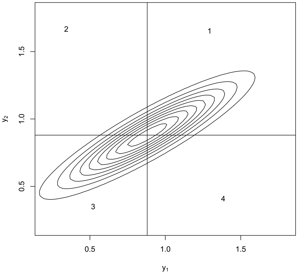
The fact that the GLS estimate is the BLUE estimate (and also the MVUE estimate if the data is Gaussian) and that it lies below the range of (y1, y2) suggests two features. First, μ must be likely to fall outside the range of (y1, y2). Second, there must better than random chance capability to guess on which side of the range of (y1, y2) that μ lies.
In addition to GLS's BLUE property, we can add support for GLS by numerical example to illustrate features one and two. Figure 1 plots the contours of the bivariate normal density having Σ given by Equation 1 and μ = 0.88 which as shown previously is the OLS estimate of the mean in the case y1 = 1.5 and y2 = 1.0. Informally, we can integrate this density over regions 1 and 3 to see that there is a large probability that both y1 and y2 lie either above the mean or below the mean, so indeed μ is likely to fall outside the range of (y1, y2). Integration of the bivariate normal for Σ given by Equation 1 indicates that with probability approximately 0.40, μ lies below the minimum of (y1, y2) and with the same probability μ lies above the maximum of (y1, y2). This is a total of approximately 0.80 probability that μ falls outside the range of (y1, y2), which is an example of feature one. Having an estimate lie outside the range of the data is therefore defensible, provided (feature two) that one can guess with better than random chance performance whether μ lies below the minimum or whether μ lies above the maximum of (y1, y2). To see that one can beat random guessing performance, suppose y1 > y2 as in our case (y1 = 1.5 and y2 = 1.0). Then, because is larger than in Equation 1, μ is more likely to fall below y2 because if instead μ > y1 then the distance from y1 to μ would be smaller than the distance from y2 to μ, contradicting the fact that . To confirm this line of reasoning, in 10,000 simulations (in the statistical computing language R) of (y1, y2) pairs having μ = 0.88, 57% of the simulation runs for which y1 > y2 did in fact also have μ < y2. On the basis of 10,000 simulations, 57% is repeatable to within ± 1% or less, so this is better than random chance (50%) guessing. This is not a formal proof but does suggest a direction to understand when a GLS estimate falling outside the range of the data is effective. Note that y1 = 1.5 and y2 = 1.0 in the PPP statement, and the GLS estimate is μ̂ = 0.88 < y2.
5. Example Where PPP Occurs without Approximation
Thus far we have not demonstrated any error model which exactly (without approximation) produces a Σ that leads to PPP. A situation that leads to PPP without the approximations in Equation 1 is expressed in Theorem 3.
Theorem 3
Suppose m1 = μ + ∊R1 and m2 = μ + ∊R2 where ∊R1 is random error in m1 with variance and similarly for ∊R2. Then if y1 = m1 + ∊S and y2 = m2 + α∊S, where ∊S ∼ N(0, σS) and α is any positive scale factor other than 1, the covariance matrix Σ of (y1, y2) can lie in the PPP region.
Proof
The proof is by demonstration. Specify any values σ1, σ2, and σ12 that satisfy the PPP condition . Choose any α > 0, then , , and . As an example, let , , and as in Equation 3. Then if α = 0.7, we have , , and .
Note:
If α = 1, then Σ has the form of Equation 11, so PPP cannot occur ([2]).
If α < 0 then PPP cannot occur. However, our applications have α > 0. Jones et al. [10] showed that if ρ → ±1 and σ1 ≠ σ2, then μ can be estimated with surprisingly small variance. That fact plus the known BLUE property of GLS could convince us to just “live with” the PPP because it can make sense for the GLS estimate μ̂ to lie outside the range of (y1, y2) in the case α > 0, or σ12 > 0.
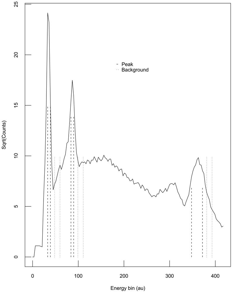
One example in which the assumptions of Theorem 3 hold involves subtracting a background measurement from a region of interest (ROI) measurement to get a net result. Because the background measurement often involves a different number of channels than the ROI measurement, a scale factor k is introduced to estimate the net counts as net = peak − k × background. Figure 2 illustrates a hypothetical example where each of three peak ROIs have a corresponding background measurement in the plot of the square root of detected neutron counts versus neutron energy in arbitrary units (au).
Suppose each ROI and corresponding background are analyzed separately, and consider the first ROI in Figure 2. The count times could vary between the two experiments, so . Both experiment 1 and experiment 2 measure the ROI counts, but in many situations, the background measurement is made only by experiment 1. In that case, experiments 1 and 2 must use the background measurement made by experiment 1. Also, if the ROI is found by analyzing the shape of the curve (the “spectrum”) that describes detected count rates versus particle energy, then the ROI for experiments 1 and 2 could differ. We then have N1 = G1 − a1 × B and N2 = G2 − a2 × B, where N is net counts, G is gross counts, B is background, a1 is the scale factor for experiment 1, and a2 is the scale factor for experiment 2. The scale factor a1 for experiment 1 is the ratio of the number of ROI channels to the number of background channels, and similarly for the scale factor a2 for experiment 2. The channel counts have variation from repeat to repeat so the detected counts will vary around the true counts with some error. As an aside, often the channel counts have approximately a Poisson distribution which for large count rates is well approximated by a Gaussian distribution. Regardless of which probability distribution best describes the channel counts, there are measurement errors in N1, N2, and one can divide N1 = G1 − a1 × B by a1 to convert this pair of equations to those assumed in Theorem 3.
6. Conclusions
Because Peelle's original statement is vague, there have been several interpretations and solutions. In our experience, there is considerable variation among experimentalists in the expression of measurement uncertainty, and a wide the range of analyses can result from vague uncertainty statements.
The three main contributions of this paper are: (1) illustrating examples when PPP cannot occur (Theorem 1); (2) providing insight when PPP is effective and appropriate (related to Theorem 2), and (3) deriving a realistic covariance matrix Σ for which PPP occurs according to physical descriptions of realistic measurement scenarios (Theorem 3). We also showed via numerical integration that an estimate lying outside the range of the data is sensible. This is because the unequal variances of x1 and x2 provide information regarding whether μ is more likely to be less than the minimum or greater than the maximum of x1 and x2.
Of course GLS provides a good estimate μ̂ in general because of its well-known BLUE property (and MVUE if the data is Gaussian) and in particular for the PPP problem if the covariance Σ is well known.
There will almost always be estimation error in Σ̂, and often the measurement errors are nonGaussian. Therefore, we consider the following two topics in [6]: (1) alternatives to GLS when there is estimation error in Σ̂, and to provide estimators other than GLS that use the estimated likelihood in the case of non-Gaussian error models that make ML estimation difficult. Regarding (1), it is known that weighted estimates do not always outperform equally-weighted estimates when there is estimation error in the weights. We have already noted that estimation of Σ in Equation 1 introduces apparent PPP when PPP does not actually occur.
Finally, [10] showed that when the diagonal entries in Σ are different and the correlation is large and positive, the GLS estimate can have lower variance than if the correlation is zero. This fact does not seem to be widely known, and experimental opportunities to exploit this fact are under investigation.

Acknowledgments
We acknowledge the next generation safeguards initiative within the U.S. Department of Energy.
References
- Peelle, R. Peelle's Pertinent Puzzle; Oak Ridge National Laboratory Memorandum: Washington DC, USA, 1987. [Google Scholar]
- Nichols, A.L. International Evaluation of Neutron Cross Section Standards; International Atomic Energy Agency: Vienna, Austria, 2007. [Google Scholar]
- Chiba, S.; Smith, D. A Suggested Procedure for Resolving an Anomaly in Least-Squares Data Analysis Known as Peelle's Pertinent Puzzle and the General Implications for Nuclear Data Evaluation; Report ANL/NDM-121; Argonne National Laboratory: Argonne, IL, USA, 1991. [Google Scholar]
- Zhao, Z.; Perey, R. The Covariance Matrix of Derived Quantities and Their Combination; Report ORNL/TM-12106; Oak Ridge National Laboratory: Oak Ridge, TN, USA, 1992. [Google Scholar]
- Hanson, K.; Kawano, T.; Talou, P. Probabilistic Interpretation of Peelle's Pertinent Puzzle. Proceeding of International Conference of Nuclear Data for Science and Technology, 26 September–1 October 2004; Haight, R.C., Chadwick, M.B., Kawano, T., Talou, P., Eds.; AIP Conference Proceedings: Melville, NY, USA, 2005. [Google Scholar]
- Burr, T.; Kawano, T.; Talou, P.; Hengartner, N.; Pan, P. Alternatives to the Least Squares Solution to Peelle's Pertinent Puzzle. submitted for publication. 2010. [Google Scholar]
- Christensen, R. Plane Answers to Complex Questions, The Theory of Linear Models; Springer: New York, 1999; pp. 23–25. [Google Scholar]
- Burr, T.; Frey, H. Biased Regression: The Case for Cautious Application. Techometrics 2005, 47, 284–296. [Google Scholar]
- Sivia, D. Data Analysis—A Dialogue With The Data. In Advanced Mathematical and Computational Tools in Metrology VII; Ciarlini, P., Filipe, E., Forbes, A.B., Pavese, F., Perruchet, C., Siebert, B.R.L., Eds.; World Scientific Publishing Company: Lisbon, Portugal, 2006; pp. 108–118. [Google Scholar]
- Jones, C.; Finn, J.; Hengartner, N. Regression with Strongly Correlated Data. J. Multivariate Anal. 2008, 99, 2136–2153. [Google Scholar]
- Finn, J.; Jones, C.; Hengartner, N. Strong Nonlinear Correlations, Conditional Entropy, and Perfect Estimation. In Bayesian Inference and Maximum Entropy Methods in Science and Engineering, Proceeding of 27th International Workshop Bayesian Inference and Maximum Entropy Methods in Science and Engineering, Saratoga Springs, NY, USA, 2007; AIP Conference Proceedings: Melville, NY, USA, 2007; p. 954. [Google Scholar]
© 2011 by the authors; licensee MDPI, Basel, Switzerland. This article is an open access article distributed under the terms and conditions of the Creative Commons Attribution license (http://creativecommons.org/licenses/by/3.0/.)
Share and Cite
Burr, T.; Kawano, T.; Talou, P.; Pan, F.; Hengartner, N. Defense of the Least Squares Solution to Peelle’s Pertinent Puzzle. Algorithms 2011, 4, 28-39. https://doi.org/10.3390/a4010028
Burr T, Kawano T, Talou P, Pan F, Hengartner N. Defense of the Least Squares Solution to Peelle’s Pertinent Puzzle. Algorithms. 2011; 4(1):28-39. https://doi.org/10.3390/a4010028
Chicago/Turabian StyleBurr, Tom, Toshihiko Kawano, Patrick Talou, Feng Pan, and Nicolas Hengartner. 2011. "Defense of the Least Squares Solution to Peelle’s Pertinent Puzzle" Algorithms 4, no. 1: 28-39. https://doi.org/10.3390/a4010028