1. Introduction
In many real-time embedded systems, some form of scheduler is generally used instead of a full “real-time operating system” to keep the software environment as simple as possible. A scheduler typically consists of a small amount of code, and a minimal hardware footprint (e.g., a timer and interrupt controller). In this context, a scheduler is a basic component of an embedded system architecture that is primarily employed to assign (or ‘dispatch’) software tasks to CPU’s at run-time. In a typical situation, at any given time there will be more tasks than CPU’s available; the role of the scheduler is to assign tasks to CPU’s such that some design goal is met. This paper is concerned with single-processer scheduling, in which there are several periodic tasks to be dispatched on a single CPU, and the goal is to schedule the tasks such that deadlines are not missed. An example of such a situation would be a processor employed in a critical application such as automotive/avionic control and robotics. In such a situation, ‘late’ calculations—
i.e., deadline misses—may lead to system instability, resulting in damage to property or the environment, and even loss of life [
1].
In general, a scheduler for such a system may be designed around several basic paradigms: time-triggered or event-triggered, and preemptive or co-operative (non-preemptive) [
1,
2,
4,
5]. This paper is primarily concerned with time-triggered, co-operative (TTC) schedulers. TTC architectures have been found to be a good match for a wide range of low-cost, resource-constrained applications. These architectures also demonstrate comparatively low levels of task jitter, CPU overheads, memory resource requirements and power consumption [
2,
3,
4,
5]. Additionally, exploratory studies seem to indicate better transient error recovery properties in TTC systems over their preemptive counterparts; however this issue requires much further investigation [
6,
7].
However, non-preemptive schedulers also have certain well discussed drawbacks over their preemptive counterparts; a presumed lack of flexibility, an inability to cope with long task execution times and long/non-harmonic periods, and fragility/complexity problems when generating a schedule being the main perceived obstacles [
3,
5,
8,
10]. In practice several techniques now exist to help overcome some of these problems. For example, co-operative designs based on well-understood patterns and state machines [
9] coupled with pre-runtime scheduling techniques [
4] provide good working solutions to the ‘long task’ problem.
The simplest form of practical TT scheduler is a “cyclic executive” [
2,
3,
8]. Cyclic executives achieve their behavior by storing a (repeating) look-up table which controls the execution of jobs at any instant of time. The lookup table is divided into a number of minor cycles, which make up a major cycle; the current minor cycle advances with each timer ‘tick’. Such a model is generally effective when all task periods are harmonically related, resulting in a short major cycle length. It is known that the off-line problem of assigning task instances to minor cycles (
i.e., creating the lookup table), such that periodicity constraints of the task are respected, is NP-Hard [
8]. However, several effective techniques—such as those adapted from bin packing and simulated annealing—have been developed for most small instances of the problem [
8].
A clear limitation that can arise in such architectures is as follows; the major cycle length is proportional to the least common multiple of the task set periods. Thus, when arbitrary - as opposed to harmonic - task periods are considered, no sub-exponential bound can be placed on the length of the required major cycle. In these cases the amount of memory required for storing the lookup table, and the resulting computational resources that are needed to design the schedule, become hugely impractical. Therefore heavy restrictions have to be placed on the choice of task set periods.
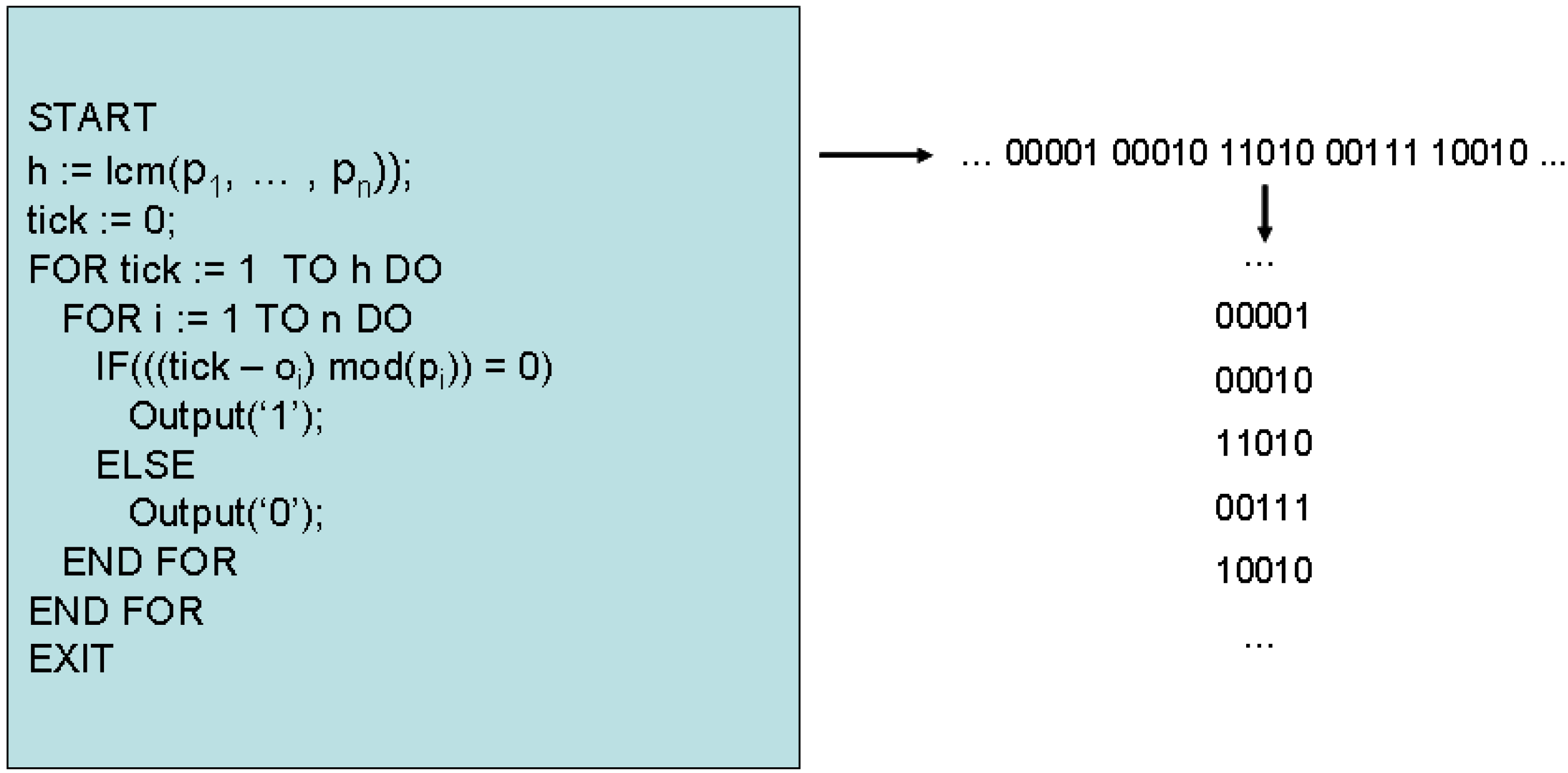
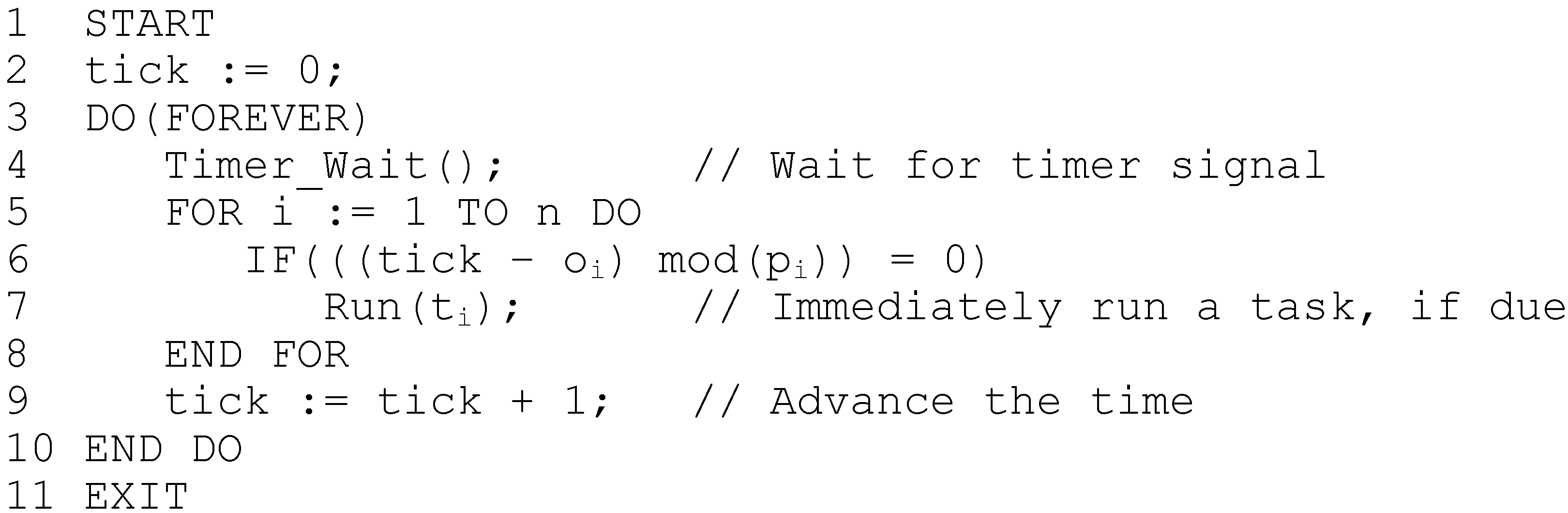
To overcome this limitation, the non-preemptive ‘thrift’ scheduler (or ‘TTC’ scheduler) has been proposed [
9]. This scheduling algorithm does not allow the use of inserted idle-time, and essentially maintains a system of congruences to replace the lookup table, and is presented in pseudo code in
Figure 1. As can be seen, when tasks are released by the scheduler, they are immediately dispatched on a first-come, first-served basis (FCFS). In general, generating a feasible schedule for a thrift scheduler reduces to assigning offsets (delays) to each task [
9,
10], resulting in an asynchronous schedule. However, previous investigations into the complexity of deciding the feasibility of asynchronous schedules have shown it to be a strongly coNP-Complete problem, at least in the case of the preemptive schedulers [
11]. Moreover, as Goossens [
12] has commented, when attempting to assign offsets to preemptively schedule a task set, that there seems to be no way to avoid enumerating and searching an exponential amount of offset combinations; in fact the decision version of this particular problem is known to be complete for Σ
2p, even when preemption is allowed [
11]. Unsurprisingly, similar results have been demonstrated for the non-preemptive thrift cyclic scheduler, in which certain task parameters are allowed to be either integer or fractional [
20,
21].
Figure 1.
Thrift scheduling algorithm, in pseudo-code.
Figure 1.
Thrift scheduling algorithm, in pseudo-code.
The thrift scheduling algorithm has also been suggested for use in domains other than that of embedded systems, for example the processing of information requests in mission critical security applications [
22], and the underlying model has also proved to be identical (in most aspects) to scheduling problems described in other application areas, for example the periodic vehicle delivery problem [
23]. The underlying concept in these formulations is that there exists a periodic (indefinitely repeating) system of actions to be performed (tasks to execute, information to be serviced, items to deliver) in which the temporal separation of actions must
exactly correspond to the actions’ periodicity requirements; the optimization goal is to assign individual start times (‘offsets’) to each action, such that the number of actions to be simultaneously performed over the system lifetime is minimized.
The application of heuristics for this assignment of offsets in such problems—for example using greedy approaches such as the ‘First-Fit Decreasing’ (FFD) algorithm—is an attractive option; a severe drawback of recent works has been the limitation that in each step of the FFD procedure, it is required to evaluate the quality of a partial candidate solution; which is itself strongly coNP-Hard [
20]. In most cases, previous studies have severely limited the choice of task periods to attempt to circumvent this problem. For example, in [
10] Gendy & Pont describe a heuristic optimization procedure to generate feasible thrift schedules. Although the technique works reasonably well in practice, it is required to limit the ratio of minimum to maximum periods in the task set to 1:10. A similar restriction on periods is enforced by Goossens [
11], who investigates heuristic methods for preemptive schedules. In other domains, similar restrictions are placed on the various parameters in question [
22,
23]. For many applications, this restriction is clearly unrealistic. Although it has been argued that in many cases, a task set with either coprime or non-harmonic periods is not representative of real-world applications (e.g., [
10,
14])—this is true only for closely related transactions, such as filtering and updating a single control loop. In reality, for economic, topological and efficiency reasons, a single processor may well be performing multiple—not physically related—functions. As such, the periods are dictated by many factors and there is likely to be little, if any, harmonic coupling between transactions [
5,
8].
If thrift scheduling is therefore to be employed in more realistic and representative situations, then fast and effective algorithms to both decide feasibility and assign task offsets are required. This forms the main motivation for the current research. The remainder of the paper is organized as follows.
Section 2 presents the task model, defines the problem and reviews its complexity.
Section 3 describes the Largest Congruent Subset (LCS) algorithm, which significantly improves upon previous algorithms for the feasibility problem. In
Section 4, exact and approximate methods for solving the offset assignment problem are described, along with a discussion of how offset symmetries can be efficiently broken.
Section 5 presents detailed results of computational experiments to investigate the performance of the new algorithms.
Section 6 concludes the paper and suggests areas for further research.
3. Algorithm for TSAFP
3.1. Basic Idea
The basis for a new algorithm starts from a single requirement; given the thrift scheduling algorithm (as shown in
Figure 1) and an asynchronous task set
τ, determine - in the fewest possible steps—the correct value of
cMax. In order to find this value in the fewest possible steps—in a manner that is robust to the task set periods—the possibility of examining task phasings is explored. Since the scheduler controls the release of each task, and tasks can only be released at the start of each tick interval, the scheduler can be viewed purely as a generator of an equivalent binary sequence, as follows. Given the task parameters
τ, the scheduler produces
h n-bit long binary sequences, one for every tick interval; where a ‘1’ in each sequence indicates that the corresponding task is released at this tick, and a ‘0’ represents otherwise. This abstraction is illustrated in
Figure 3, for a 5-task system.
Figure 3.
Thrift scheduling as binary sequence generation.
Figure 3.
Thrift scheduling as binary sequence generation.
In such an abstraction, the demand for processor time η at each tick interval relates to this binary sequence as follows. The processor demand at the kth tick interval is determined by simply weighting the ith binary digit in the kth n-bit sequence by the ith task’s execution time, ci, then summing the weighted totals. To observe the worst-case behavior of a given schedule, it follows from Theorem 1 and Equation (7) that h n-bit long binary sequences must be examined. In general, from (7), it can be observed that from the numerical properties of least common multiple, in the worst-case h is proportional to the product of the task set periods (this situation occurs when all periods are pairwise coprime). If the maximum of the task set periods is represented by the parameter pmax, it follows that the running time of a hyperperiod simulation algorithm is given by O(n pmaxn). It can also be observed that in the best case—for instance when all task periods are restricted to be integer powers of 2 (2, 4, 8, 16, 32 … etc.)—h is simply proportional to pmax; the best one can hope for is that the algorithm running time is pseudo-polynomial in the input parameters.
It may seem that a useful restriction to consider would be to place an upper bound on the choice of periods—say in the interval [1,50]—but this can still result in a length of h that can approach 1038. In most cases, a more realistic restriction would be to suppose time is represented in milliseconds, and tasks may require periods in the interval [1, 1,000]. It is trivial to create instances in which number of tasks is small (e.g., ≤30), and the length of h exceeds 10100 with this more realistic restriction. It can be observed then, that the actual time complexity of deciding a given PSD problem instance is incredibly fragile, and is highly dependent on the task periodicity requirements.
However, consider a parameterization of the input representation, which primarily considers the number of tasks
n and the largest task period
pmax (the remaining task parameters may be neglected from this analysis as they do not affect algorithm run times). Now, in a system with
n tasks, there is a maximum of 2
n possible binary combinations of tasks, the actual patterns which will be generated by the scheduler at run time depend on the choice of offsets; for almost all instances of this problem, 2
n <<
h. For example, consider a system of 10 tasks with periods in the interval [1, 1,000]. Whilst
h may approach 4 × 10
20 in such a situation, 2
n is significantly smaller—1,024—in comparison. In most real-world instances of the problem,
n will in fact be relatively small (e.g., ≤ 30). This observation forms the basis for the LCS algorithm; if an algorithm can be developed such that the running time is exponential only in the number of tasks
n, and polynomial in the representation of
pmax, this will be a marked improvement in efficiency in most cases; it will in fact constitute a fixed-parameter tractable (FPT) algorithm in the sense described by Niedermeier [
25]. In order to explore this possibility further, the nature of congruencies in a periodic system of tasks will be explored.
3.2. Congruence of Periodic Tasks
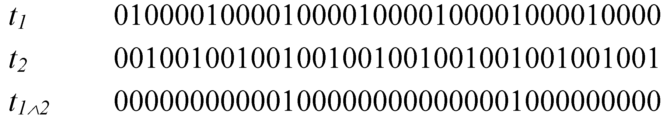
Consider two tasks
t1 and
t2 represented purely as binary sequences. This is shown in
Figure 4 for the case where
p1 = 5 and
p2 = 3, with offsets of
o1 = 1 and
o2 = 2. The coincident task releases (logical AND) are also indicated, where a ‘1’ indicates that the two tasks are released (phased) together.
Figure 4.
Congruence relationship of two periodic tasks.
Figure 4.
Congruence relationship of two periodic tasks.
Given the thrift scheduling algorithm, each task can be represented as a linear congruence of the form:
where
x is one of the (multiple) possible solutions to the congruence. If the two tasks are phased together (denoted by
φ(t1, t2)) then
x must be a valid integer solution to both congruences simultaneously. According to the
linear congruence theorem this occurs iff:
That is, if the relative offsets of the tasks divides the
gcd of the periods. Suppose now that we wish to consider the phasing of a set of
m tasks. Clearly,
x must now provide a valid solution to each of the
m simultaneous congruences for the tasks to all be in phase. According to the
Chinese remainder theorem [
12,
18], (12) can be extended such that a valid integer solution to such a set of
m congruences exists iff:
That is, if each pair wise combination of tasks in the set
m satisfies (12) simultaneously. In such a case that each pair wise combination of periods in
m are coprime then (13) is guaranteed to be true. Equations (12) and (13) form the basis for the LCS algorithm. A
congruent subset is defined as a set
T ⊆
τ s.t. ∀
i,j ∈
T, equation (13) holds. Let |
T| be the cardinality of the subset,
i.e., the number of tasks it contains, and let (
T) refer to the magnitude of the subset:
The purpose of the LCS algorithm is to search for a congruent subset of tasks with the largest magnitude, given an asynchronous task schedule. Central to the proposed algorithm is the notion of a phase matrix ϕ. This is an n-by-n matrix that contains all pairwise task phasing information, encoded in binary format. For all elements i,j, j > i, a ‘1’ is placed in the ijth element of the matrix indicating a phasing of tasks i and j, and a ‘0’ indicating otherwise. The matrix is ‘0’ both on and below the diagonal, and can be generated by repeated application of the gcd algorithm and Equation (12) to each pair wise combination of tasks in the set, and effectively defines the powerset of all possible task phasings. Each row of this matrix is referred to as a ‘phase code’, and represented as an n-bit long binary string; in this paper, each phase code is represented as an unsigned integer. The phase code Pj corresponds to the jth row of the phase matrix ϕ.
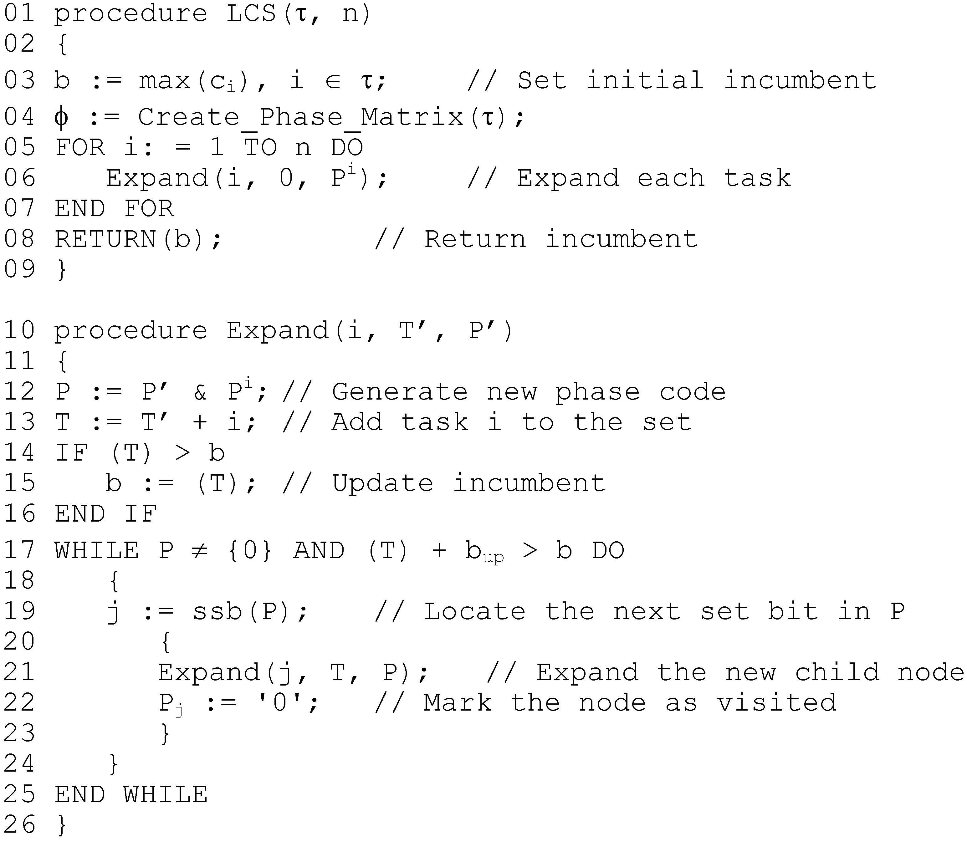
3.3. Algorithm Description
The LCS algorithm (Please note that an earlier for the LCS algorithm was previously described by the current author in [
21]) operates as a depth-first search of all possible task phasings, employing simple bounding heuristics to help prune the search. The inputs to the algorithm are a task set
τ, and the output of the algorithm is the determined value of
cMax. The first step is the calculation of the phase matrix. The initial incumbent solution value
b is set to the maximum of the largest task execution times, and summed execution times of any pairwise phased tasks during this process;
cMax cannot be any less than this. The algorithm then begins to recursively search for congruent subsets of tasks; the main elements of the algorithm are shown in
Figure 5.
Each node of the search tree represents a subset T of congruent tasks; the depth of recursion corresponds to |T|. The incumbent is updated whenever a subset with (T) > b is found. Each node has associated with it its own phase code P. Since only proper congruent subsets can be expanded as child nodes in the search, the ith task can only be added into the current subset T to form a new child node with subset T’ if the ith bit of P is set to a ‘1’. To generate the new phase code in the child node, a logical AND is performed between P’ and Pi, the ith row of the phase matrix. This effectively applies equation (13) in one single operation, and the only bits that will subsequently be set to ‘1’ in P thus correspond to tasks that are properly congruent with all tasks in T. When an empty phase code is encountered, the algorithm begins to backtrack since either a leaf node has been reached or - since bits are cleared by the algorithm after the corresponding child node has been explored – no further child nodes exist.
Figure 5.
LCS algorithm, in pseudo-code.
Figure 5.
LCS algorithm, in pseudo-code.
The call to sub-function
ssb on line 19 locates the next lowest set bit in the current phase code; since these codes are represented as bit-strings, this can be performed in small fixed constant time, e.g. using techniques based around a deBruijn sequence [
24]. The pruning rule that is implemented simply prevents the expansion of child nodes which cannot possibly lead to a value greater than the current incumbent. This simple procedure works as follows; suppose the current node represents a subset
T, and that a proper child node corresponding to the
jth task is about to be expanded. An upper bound
bup on the best possible value that can be achieved by such an expansion is as follows:
This bound expresses the fact that the best possible situation - in which all tasks corresponding to unexplored branches - are congruent to T. If this value is not greater than b, then the node need not be expanded. Moreover, since the search progresses in a depth-first, left-to-right search, the current node can be considered fathomed; this bound can only be non-increasing for all child nodes greater than j. This fathoming rule, along with the fact that the algorithm can be implemented entirely using (fast) integer arithmetic, leads to a very efficient formulation. After first showing that the algorithm completely solves the TSAFP, its time complexity is analysed.
Theorem 3:
Algorithm LCS exactly solves the search version of TSAFP.
Proof:
By inspection. It can be seen that LCS will recursively enumerate only congruent subsets of tasks as the search progresses, as follows; line 12 ensures that only subsets of tasks that conform to (14) are considered as valid child nodes in the search, and the IF statement of line 20 ensures that only these nodes are actually expanded. The WHILE statement on line 18 ensures that the algorithm will explore every possible child node, backtracking iff either no unexplored child nodes remain or the current node has been fathomed according to (15). The conditional assignment on lines 15 and 16 ensure that the incumbent is only updated when the magnitude of the proper congruent subset (T) corresponding to the current node exceeds the current incumbent value b. Upon termination, the incumbent b clearly corresponds to the correct value of cMax.
3.4. Complexity
The analysis starts with the generation of the phase matrix. It can be seen that with a set of
n tasks, there are exactly 0.5
n ×
n+1 combinations of task pairs. To generate the matrix, each pair requires an application of the
gcd calculation and application of (15). If the periods in question can be encoded in log
2(p
max) bits, generation of this matrix has time complexity
O(n2 ┌log2(2pmax)┐) [
18]. Thus the computation of the phase matrix runs in time polynomial, and need only be calculated once and memoized. Moving now onto the main body of the algorithm, it can be seen from its formulation that in the worst case it is exponential in the number of tasks
n, with complexity
O(2n). However, the running time of the algorithm is clearly independent of the choice of task periods and
pmax; for any fixed
n, |2
n| is constant; LCS therefore constitutes a polynomial-time algorithm for the search version of TSAFP for fixed
n. If
n is less than or equal to the binary bit-width of the solving machine, then as mentioned previously the application of equation (13) can be performed with a single binary conjunction instruction; the running time of the algorithm can be described as follows:
where
f(n) is equal to 2
n. LCS thus constitutes a FPT algorithm for TSAFP, in the sense described by Niedermeier [
25]. In the more general case, it can be observed that LCS may also be applied to solve the underlying SIMULTANEOUS CONGRUENCES problem; when
n is larger than the bit width of the solving machine, the running time will be proportional to
f(n).n, which is also FPT for a given
n. As will be subsequently demonstrated, for values of
n ≤ 30—such as for the real-world task sets considered in this paper—the LCS algorithm provides an exponential running time improvement over hyperperiod simulation. The adoption of LCS has allowed for deeper investigations into the offset assignment (TSOAP) problem; attention is now focused on this problem in the following Section.
4. Algorithms for TSOAP
A simple, exact algorithm for the TSOAP problem would be as follows: enumerate and search all possible offset combinations, using the LCS algorithm to determine the optimal value of
cMax. This can be improved upon by generating an initial heuristic solution of reasonable quality, and using this solution to guide a simple back stepping search, similar to the procedure outlined in [
15]. Further improvements can be gleaned by omitting redundant configurations of offsets from the search; this is discussed in the next Section.
4.1. Breaking Symmetry
Symmetry, in the current context, occurs when two sets of task offsets O and O’ result in identical periodic behavior over the hyperperiod h, the only difference being the relative start point of the schedules at t = 0. In such cases, the value of cMax for both schedules is identical. A simple example can illustrate the concept of symmetry: suppose we have two tasks with periods {3,5}. Although offsets in the range 0–2 and 0–4 can seemingly be considered, the periods are coprime; all choices of offset are in fact identical and result in the same periodic behavior, shifted only at the origin. Obviously, to reduce the search space it is wished to only consider one set of offsets in situations where symmetry exists.
Previous work in the area of offset-free preemptive scheduling by Goossens [
11] has shown that in most periodic task system in which one is free to assign offsets, many classes of equivalent offset combinations exist. It is clear from the proofs developed in this previous work (specifically Theorem 9) that this can be also be shown to hold for the case of the offset-free non-preemptive thrift scheduler. [
11] also outlined a method to break symmetries as part of a backstepping search algorithm; this can be adapted to develop a simple polynomial-time symmetry breaking algorithm, which is called once (and once only) before a search begins. Also, this method does not require the manipulation of any large integers—which in practice causes integer overflow even for moderately low
n—and is also somewhat faster in practice.
Let
p’ be the
phase capacity of a task, which is used to place an upper bound on the choice of its offset, such that if offsets for task
i are selected in the range 0 ≤
oi <
p’ then all (and only) redundant configurations of offsets will be removed from the search. Since the evaluation of each offset configuration in the search space requires the solution of a coNP-Hard problem, this clearly has many benefits. For the first task,
p’ is always zero; this follows from Theorem 6 in [
11]. For all 1 <
i ≤
n,
p’ can be calculated as the
lcm of the pairwise
gcd’s between task
i’s period, and all other periods less than
i:
Theorem 4:
Considering task offsets upper bounded by p’ only removes all (and only) redundant offset configurations from a search.
Proof:
Trivially follows from Theorem 10 in [
11], the definition of
p’ given by (17) and the basic numerical properties of
gcd and
lcm.
Given the complexity results outlined in
Section 2, it is unlikely that even small instances of the offset assignment problem may be solved exactly in a tractable time. In order to obtain relatively quick ‘good’ solutions to the problem, heuristics can be employed. Given the similarity of the considered problem to the multiprocessor scheduling problem, it follows that algorithms that have been useful in this area may also be applied in the current context. Before describing two such algorithms, the notion of symmetry will be extended further. In previous papers, the potential effects of symmetry on the hyperperiod of the task set have not been considered. From (12) and (13), it is clear that only the relative offsets of individual tasks define the subsets of tasks that are congruent. Thus, let the
harmonic period h’ of a task
i be defined as follows:
This is a simple extension of the notion of phase capacity. Suppose we now consider a
reduced task set
τ’, in which the tasks are identical to those in
τ, with the exception that each and every period
p is replaced by
h. Such a reduced task set would then have a
reduced hyperperiod hr defined as follows:
Equation (18) defines a hyperperiod that contains no symmetries; since hr ≤ h (and in most cases hr << h) an alternative formulation to decide TSAFP would be to perform hyperperiod simulation using τ’. To show that such an algorithm is proper, from (12) and (13) it would need to be shown that τ’ contains all (and only) those task congruences that are present in τ.
Theorem 5:
τ’ contains all (and only) those task congruences that are present in τ.
Proof:
By showing that gcd(p1, p2) = gcd(h1, h2). Let x = gcd(p1, p2) and y = gcd(h1, h2). From (18) and by the definition of lcm, we have h1 = ax and h2 = bx, where a and b are some positive (non-zero) co-prime integers. Then we have y = gcd(ax, bx); since a and b are co-prime, by definition gcd(ax, bx) = x. Since we have that in fact y = x, the Theorem is proved.
This shows that all task congruences are preserved by using such a method, and no further congruences are introduced. It can be noted that this also gives a fast and effective way to detect instances which can be decided rapidly using traditional means, for example equivalent synchronous systems;
i.e., those in which all periods are co-prime, or task sets with high degrees of harmonic coupling. The LCS algorithm can be modified to detect such instances as follows: if
nh’ << 2
n then hyperperiod simulation is used; else the procedure defined in
Section 3 is used. However, early experience with LCS indicates that in the average case, a more suitable test can be
nh’ <
npMax, where
pMax is the largest of the task periods.
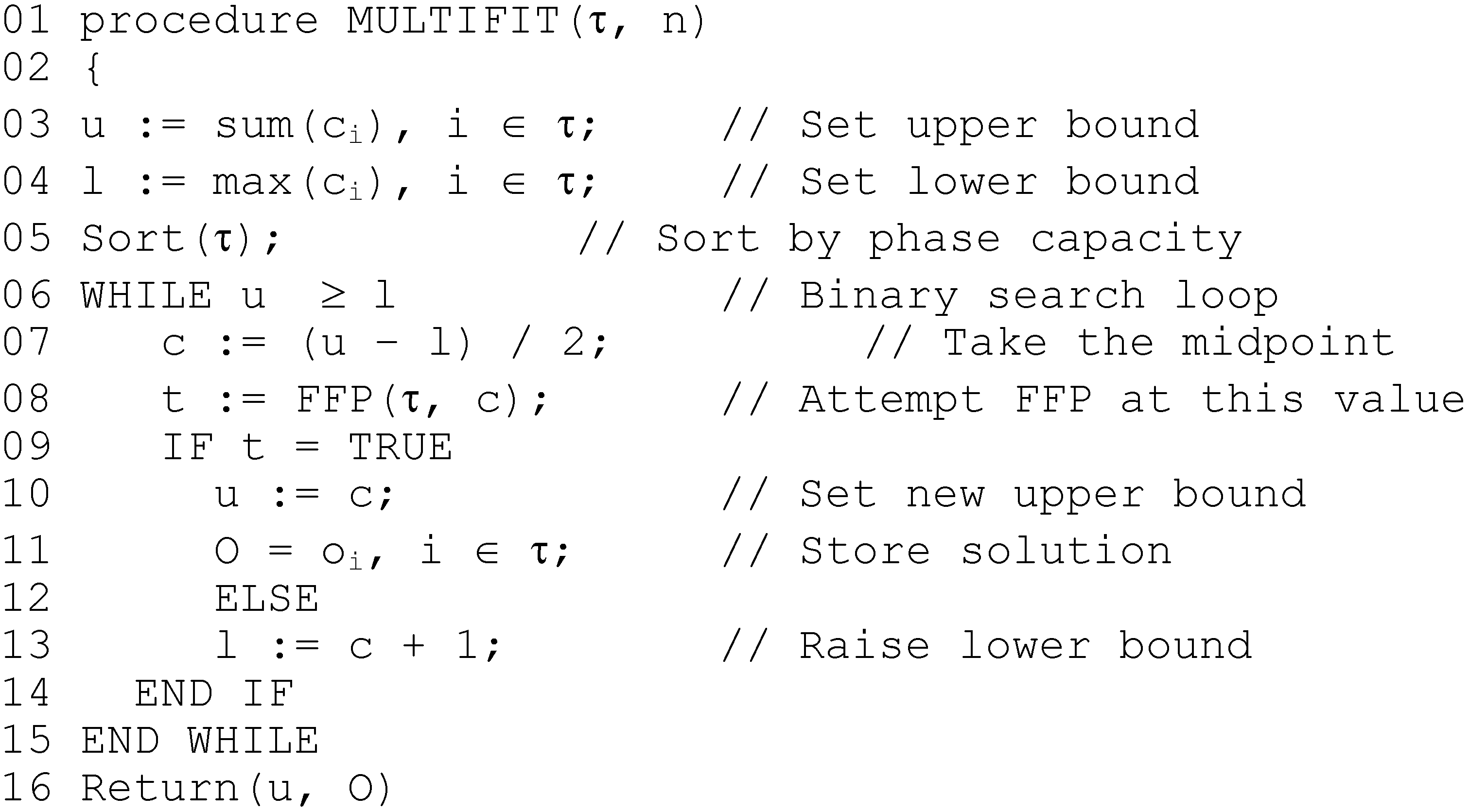
4.2. The MULTIFIT Algorithm
In [
10], the authors suggest a basic heuristic for offset assignment, achieved by sorting the list by non-decreasing period before application of a basic First-Fit (FF) algorithm under the assumption that each successive task is ‘easier’ to fit around the previous tasks. Given the analysis of the previous Section, it is clear that a better option would be to order the tasks by non-decreasing harmonic period; this leads to the First-Fit-Phase (FFP) algorithm. FFP first performs such a sort, then each task is assigned—one by one—the lowest indexed offset that will schedule it, until either all task are scheduled (returning TRUE) or one or more tasks couldn’t be scheduled (returning FALSE). The LCS algorithm is used for the feasibility test, and to reduce the search space only offsets bounded by each tasks phase capacity
p’ are considered. The MULTIFIT algorithm proposed in this paper uses FPP as a key component in a binary search; MULTIFIT for the classical multiprocessor scheduling problem was originally proposed in [
13], and it has been proven that the resulting makespan can be no further than 22% away from the optimal makespan. The modified algorithm considered in this paper is very similar; a binary search is performed to find the minimum value of α such that applying FFP schedules the task set. Since FFP (and hence LCS) are called multiple times, the
gcd’s of each pair of tasks are computed once only and stored in an array, and sorting is performed once only. The initial upper bound is set to the sum of tasks execution times, and the lower to the largest execution time in the task set. The MULTIFIT algorithm proposed in this paper is shown in
Figure 6.
Figure 6.
MULTIFIT algorithm, in pseudo-code.
Figure 6.
MULTIFIT algorithm, in pseudo-code.
As mentioned, for fixed
n LCS runs in polynomial time; hence for fixed
n, MULTIFIT has complexity
O(np’max),
i.e., pseudo-polynomial. The second algorithm to be described is based upon a local-search version of the classical LPT algorithm described by Graham [
17].
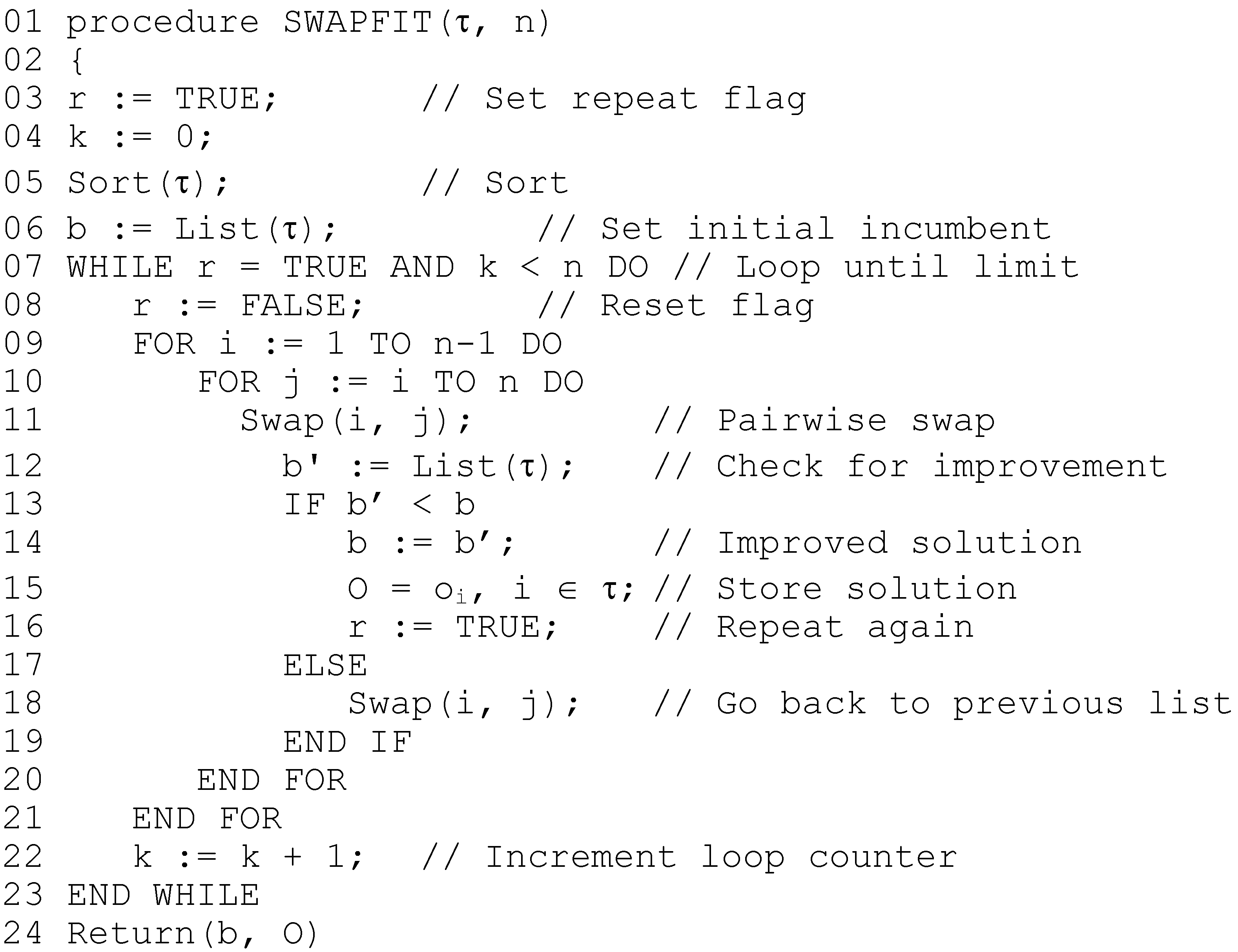
4.3. The SWAPFIT Algorithm
The LPT algorithm for multiprocessor scheduling first sorts the tasks in order of decreasing execution time, and assigns the tasks one by one onto the first available processor; the latter operation is known as list processing. It has been proven that the makespan resulting from LPT is no further than 33% from optimal. The rationale behind SWAPFIT is simple; there is a permutation of the tasks such that application of list processing produces an optimal makespan, and in [
17], it is shown that the list produced by sorting for non-increasing execution times produces a permutation that is very close to optimal. Starting from a good, initial solution, an attempt is made to sort the list into a better order, guided by resulting changes in the value of the objective function. In the SWAPFIT algorithm, list processing is modified as follows; each task in the list is assigned, one by one, an offset (bounded by
p’) that minimizes the worst-case release of the task. LPT is initially employed to obtain a starting solution. Next, every pairwise set of tasks in the list is reversed, one by one; if such a reverse causes the objective function to decrease when the tasks are list processed, it is accepted. If not, the change is rejected, and the tasks swapped back. The SWAPFIT algorithm is shown in
Figure 7.
Figure 7.
SWAPFIT algorithm, in pseudo-code.
Figure 7.
SWAPFIT algorithm, in pseudo-code.
For SWAPFIT, it can be seen that the inner loop of pairwise reversals performs approximately 0.5 n2 reverses and list processes, and this process continues until either no more beneficial changes can be made, or an upper bound on allowed iterations is reached. As with most local search techniques, no sub-exponential bound can be placed on the number of iterations of this outer loop; in practice, this seems proportional to (but significantly less than) n. By setting an upper bound as n and simply returning the best solution found if this bound is exceeded, the algorithm again runs in pseudo-polynomial time for fixed n, with complexity O(max(n3, np’max)). Since LCS is called multiple times, the gcd’s of each pair of tasks are again computed once only and stored in an array.
Before moving onto describing the computational experiments, it is worthwhile discussing performance bounds for the two algorithms. The quoted performance bounds for the original versions of both MULTIFIT and LPT are known to be extremely tight for multiprocessor scheduling [
13,
17]. However, it is clear that the performance bounds do
not hold for the current algorithms. When periods are evenly divisible, it can be seen that FFP results in a packing that is identical to First Fit (FF); however for general problem instances, no bounds are currently known. That said, it can be conjectured that both heuristics will produce a ‘good’ schedule; exactly how good this schedule is likely to be for general instances of the problem is investigated in
Section 5. A general lower bound (
zl) for the optimal value of general problem instances can be obtained through (20):
where
u is the task set utilization. However it can be observed that this bound can be arbitrarily far from the true value, simply by considering subsets of tasks with co-prime periods; it follows from the Chinese remainder theorem that no choice of task offsets can avoid them being congruent. In many cases a tighter bound can be obtained by employing LCS to determine the largest co-prime task phasing. This observation leads to an alternate formulation for exact solutions to the problem; the Iteratively Tightening Lower Bound (ITLB) algorithm.
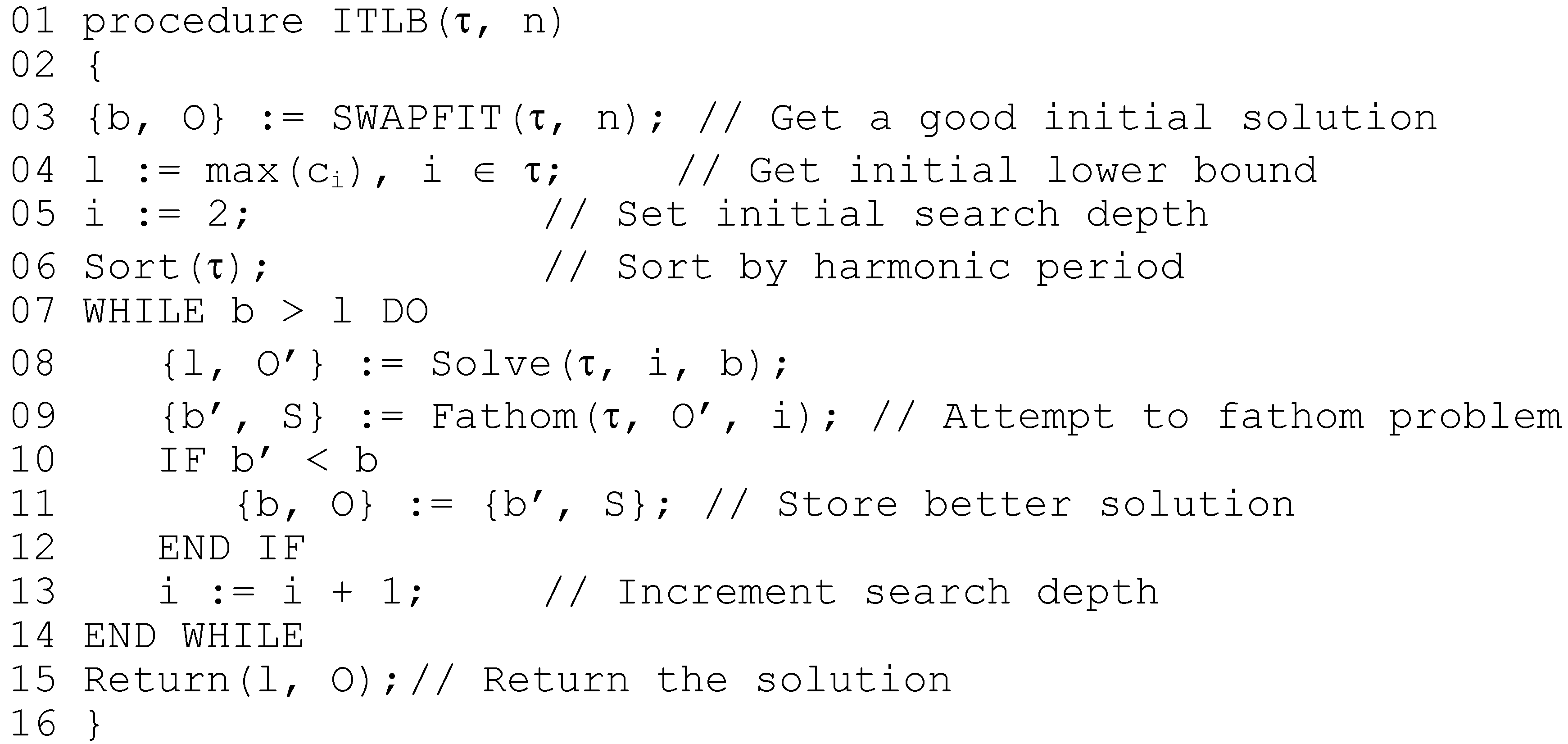
4.4. The ITLB Algorithm
The ITLB algorithm builds from the fact that in any schedule, there is a task ‘bottleneck’ that defines the optimal value achievable for the problem instance. This bottleneck is most likely to be between tasks whose pairwise
gcd’s are low; for example, a subset of tasks with co-prime periods. The ITLB algorithm works as follows; an initial incumbent solution
b is found using SWAPFIT, and the tasks are then sorted according to non-decreasing harmonic period; tasks with low harmonic period are the most difficult to separate. Then, starting with low
i, the first
i tasks are solved to optimality, with backstepping guided by
b. The optimal value
l found by this process constitutes a lower bound on
z; as the number of tasks is increased above
i, it is clear to see that
l cannot possibly decrease. Given the bound
l, and a set of offsets
O’ for the first
i tasks, the algorithm then attempts to schedule the remaining
n-
i tasks using SWAPFIT, such that the optimal value does not increase. If this can be achieved, then a provably optimal schedule has been found; if it cannot,
i is incremented to deepen the search, and
b and
l are updated if a better solution or tighter lower bound have been found, and the process repeated. The ITLB algorithm is shown in
Figure 8.
The call to Solve() on line 8 finds the best solution to the first i tasks; while the call to Fathom() on line 9 applies the heuristic to schedule the remaining tasks. It can be seen that with every iteration the lower bound is non-decreasing, and the incumbent is potentially improved; the iterations repeat until optimality is proved. In the worst case, every possible offset combination is enumerated and tested, and it is clear to see that the problem is solved exactly. However, it is also clear that the algorithm may be terminated at any point, and the best know solution returned; in addition, the deviation from this solution from the best known lower bound can also be returned. Thus, unlike regular backstepping algorithms for this and similar problems, ITLB constitutes a complete anytime algorithm for TSOAP. The following Section presents the performance data for the described algorithms.
Figure 8.
ITLB algorithm, in pseudo-code.
Figure 8.
ITLB algorithm, in pseudo-code.
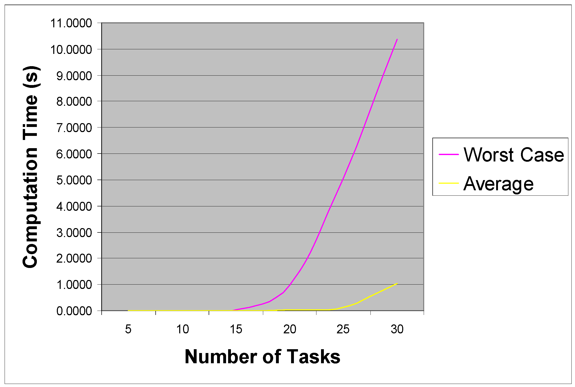
6. Conclusions
In this paper, the problem of assigning offsets to tasks in order to minimize worst-case congruent release of tasks in a thrift scheduler has been investigated, and the complexity of the problem has been shown. Several new approaches to solving the problem have been formulated; in practice both the time complexity and the performance of these algorithms seems acceptable for real-world task instances. In particular, the LCS algorithm, in conjunction with the SWAPFIT offset assignment algorithm, very quickly produces a schedule that seems to be either optimal or extremely close to it. It can also be noted that the ITLB algorithm also performs well, and may be used by system developers who wish to obtain a provably good solution within a certain time limit; initial experience indicates that even for larger instances, a solution that is within 10% of optimal can be found within 5 minutes. However, although the MULTIFIT algorithm performs well in its original problem domain, the same cannot be said for the modified version employed in this paper. An additional benefit of the algorithms developed in this paper is that they are guaranteed to find a schedule; many current tools to support thrift cyclic scheduling (and its close relatives) provide no such guarantee. Further work in this area will include deeper investigations into the performance of SWAPFIT, with further experiments employed to classify its performance. Improvements to the ITLB algorithm will also be investigated, along with the possibility of formulating an exact algorithm in which the number of offsets to be considered is proportional to O(2n). Further work will also consider algorithms for problem instances in which n > 30.
In conclusion, it has been shown that for most real-world instances of the described problem, it can be solved to near-optimality in a very acceptable time. The algorithms are relatively simple, allowing integration into existing development tools. Further work will investigate alternate approaches to solving the offset assignment problem, by using ILP techniques, and will further investigate the performance of the SWAPFIT algorithm, to explore its performance in other problem domains.


