Compound Biorthogonal Wavelets on Quadrilaterals and Polar Structures

Abstract

In geometric models with high-valence vertices, current subdivision wavelets may not deal with the special cases well for good visual effect of multiresolution surfaces. In this paper, we present the novel biorthogonal polar subdivision wavelets, which can efficiently perform wavelet analysis to the control nets with polar structures. The polar subdivision can generate more natural subdivision surfaces around the high-valence vertices and avoid the ripples and saddle points where Catmull-Clark subdivision may produce. Based on polar subdivision, our wavelet scheme supports special operations on the polar structures, especially suitable to models with many facets joining. For seamless fusing with Catmull-Clark subdivision wavelet, we construct the wavelets in circular and radial layers of polar structures, so can combine the subdivision wavelets smoothly for composite models formed by quadrilaterals and polar structures. The computations of wavelet analysis and synthesis are highly efficient and fully in-place. The experimental results have confirmed the stability of our proposed approach.

1. Introduction

In recent years, the demand of realism in computer graphics needs highly detailed geometric models. These highly detailed models challenge not only the rendering performance, but also net transmission bandwidth and storage capacities. Multiresolution modeling is an important approach to balance the need of both the accuracy of models and the cost required to process them. Among the existing multiresolution techniques, the wavelets transform is a very important tool to process the multiresolution models. Here, based on bicubic polar subdivisions, we present the novel biorthogonal wavelets scheme by applying lifting operations. Figure 1 shows the sample surface sequences with polar structures, using compound polar subdivision wavelet analysis, in different resolutions. Our wavelet scheme can offer more resolution levels to the meshes with high valence extraordinary vertices or the combinatorial structures of surfaces of revolution. Because we use local lifting operations to ensure the local orthogonalization of wavelets, the computations are fully in-place and the complexity is linear time. The in-place computation eliminates the need of auxiliary memory costs of the processing. It can be seamlessly combined with Catmull-Clark subdivision wavelets to process quadrilateral meshes with polar structures.

Figure 1. Surface sequences in different resolution: (a) original surfaces, (b) and (c) surfaces by compound subdivision wavelet analysis once and twice; (d) meshes in lowest resolution.

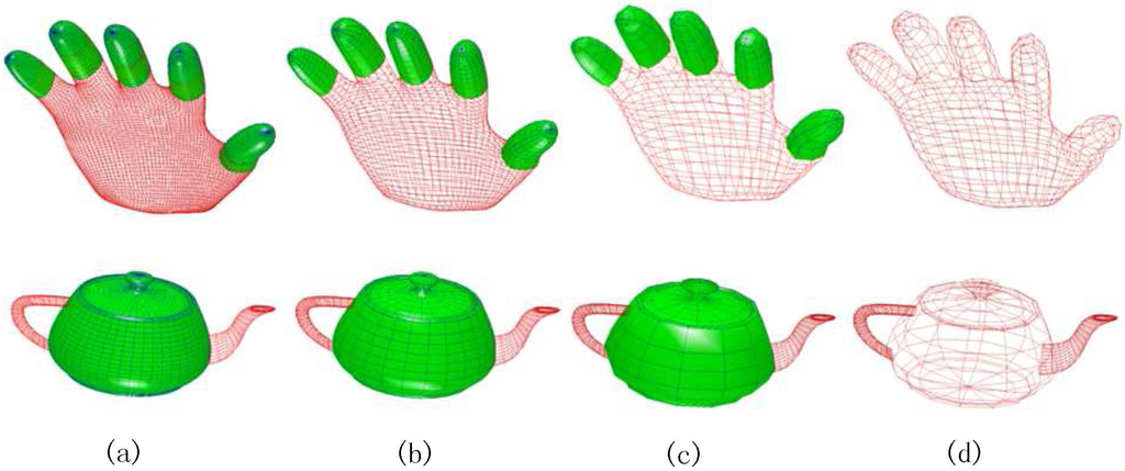
Figure 1. Surface sequences in different resolution: (a) original surfaces, (b) and (c) surfaces by compound subdivision wavelet analysis once and twice; (d) meshes in lowest resolution.

1.1. muliresolution modeling

A polygonal model M can be considered as the composition of a fixed set of vertices $V=(v_1,v_2,...,v_r)$ and a fixed set of faces $F=(f_1,f_2,...,f_n)$. It provides a single fixed resolution representation of a surface. Suppose we have a polygonal model M and we want an approximation $M^{\prime }$. While $M^{\prime }$ will have fewer polygons and vertices than the original one, it should be as similar as possible to M. A multi-resolution model is a model representation that covers a sequence of approximations of a surface and can be used to reconstruct any one of them on demand.

There are two most common methodologies in multiresolution modeling: decimation and refinement. A decimation algorithm starts from the original surface and removes elements from the model. For example, from the high detail model $M^n$, we can get a sequence of models in different levels of details by iteratively decimation.

$$M^n\to M^{n-1}\to ...\to M^0$$

In the opposition to the decimation, the refinement algorithm begins from an initial coarse approximation and adds supplements to the model. We can retrieve the high detail model $M_n$ by iterative refinement.

$$M^0\to M^1\to ...\to M^n$$

The cost of surface decimation and refinement should be low because we will often need to use many different approximations at run time. In some applications, the low cost of computation is much more important than the similarity of the objects in different resolutions.

1.2. subdivision wavelets

The subdivisions can iteratively refine a control mesh $M^0$ so that the sequence of increasingly faceted polyhedra $M^1,M^2,...$ converge to some limit surface $M^{\infty }$. The property of subdivision makes it possible to define a collection of refinable scaling functions. Based on nested linear spaces spanned by the refinable scaling functions and an inner product designated, we can construct subdivision wavelets. Subdivision wavelets not only inherit the performance advantage of wavelets in shape reservation, but also overcome the shortcomings of classical wavelets that are hardly applied in 3D domains. They can be applied on surfaces of arbitrary topology type. Comparing with subdivisions, the subdivision wavelets transform can perform both decimation and refinement operations.

The theoretical basis for constructing wavelets on subdivision surfaces was established by Lounsbery et al. [1]. They also proposed a class of subdivision based wavelets. By generalizing the uniform subdivision in topology to a new irregular subdivision scheme, Valette and Prost [2, 3] extended the work of Lounsbery et al. and proposed a wavelet-based multiresolution analysis that can be applied directly to irregular meshes whose connectivity is unchanged in the wavelet analysis. Samavati et al. [4] showed how to use least-squares data fitting to reverse subdivision rules and constructed the wavelets by straightforward matrix observations. Samavati et al. [5] constructed multiresolution surfaces of arbitrary topologies by locally reversing the Doo subdivision scheme. Khodakovsky et al. [6] developed the Loop subdivision wavelets with small support for progressive geometry compression. Since the lifting scheme proposed by Swelden [7] can generate new biorthogonal wavelets from the classic wavelets and lazy wavelets, it is an important tool to construct subdivision wavelets. Based on lifting scheme, Schröder and Sweldens showed how to construct lifting wavelets on the sphere with customized properties [8]. Using local lifting operations performed on polygonal meshes, Bertram et al. [9, 10] gave a new construction of lifted biorthogonal wavelets on surfaces of arbitrary two manifold topology and introduced the generalized B-spline subdivision-surface wavelets.

Using local lifting and the discrete inner production, Bertram [11] constructed a biorthogonal wavelet on the Loop subdivision. Li et al. [12] proposed unlifted Loop subdivision wavelet by optimizing free parameters in the extended subdivisions. Wang et al. [13] developed an effective wavelet construction based on general Catmull-Clark subdivisions and the resulted wavelets have better fitting quality than the previous Catmull-Clark like subdivision wavelets. Recently Wang et al. [14] constructed the new biorthogonal wavelets based on $\sqrt{3}$ subdivision over triangular meshes. The polar subdivision was first proposed by Karčiauskas et al. [15, 16]. Myles et al [17, 18] extended the work of Karčiauskas et al and provided the polar subdivision schemes, which can be combined with Catmull-Clark subdivision. Our work is mainly based on the scheme of Myles et al.

The rest of paper is organized as follows: The rules of bicubic polar subdivision and its reformulation are introduced in Section 2. We explain how to construct the polar subdivision based wavelets in radial/circular layers in Section 3, and show how to combine the polar subdivision wavelets with Catmull-Clark subdivision wavelet in Section 4. We present the experimental results for the wavelet analysis in Section 5. Finally, we conclude the work in Section 6.

2. Polar Subdivision

Catmull-Clark subdivision is a powerful technique widely used in representing smooth quadrilateral surface. But for many-sided blends and vertices of high valence, Catmull-Clark subdivision often generates ripples where many facets join or where features are extruded [17]. To improve the subdivision quality in this case, Karčiauskas et al. developed a new scheme called polar subdivision [16] that generalizes bicubic spline subdivision to control nets with polar structures. The polar structure is a combinatorial structure of surfaces of revolution, often appearing at points of high valence in meshes. Apart from the extraordinary vertices, the polar structure is a layer of quadrilaterals adjacent to the triangles, as shown in Figure 2. The structures naturally appears in the design of surfaces of revolution. Comparing with 4-3 subdivision, bicubic polar subdivision is more preferable for polar structures because it generates some bicubic patches in the surface as bridges which connect quads to triangles smoothly. As bicubic spline subdivision, it is natural to be combined with Catmull-Clark subdivision and can augment the capabilities of existing Catmull-Clark subdivision.

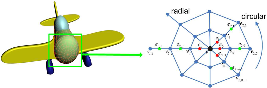
Figure 2. Polar control net near an extraordinary point. v denotes the vertex in polar net and e denotes the edge point. The control points have subscripts i which indicates the radial distance to the extraordinary point, subscripts j (modulo valence n) which indicates the circular index. $v_{1,j}$ and $e_{1,j}$ is written as $v_j$ and $e_j$ for abbreviation.

Figure 2. Polar control net near an extraordinary point. v denotes the vertex in polar net and e denotes the edge point. The control points have subscripts i which indicates the radial distance to the extraordinary point, subscripts j (modulo valence n) which indicates the circular index. $v_{1,j}$ and $e_{1,j}$ is written as $v_j$ and $e_j$ for abbreviation.

The process of polar subdivision provided by Karčiauskas et al. only includes subdivisions in radial layers. In order to apply the polar subdivision on the surface of arbitrary quadrilateral meshes, Myles et al. [17] combined the original polar subdivision with Catmull-Clark subdivision. In order to leverage and preserve the good results of radial subdivision and keep control net consistent, the subdivisions should be performed independently. It offers us a chance that the wavelet analysis in circular layers and radial layers can be constructed independently.

2.1. Subdivision in radial layers

The subdivision in radial direction is the key procedure to map a polar structure to a refined version. The refinement rules in radial layers for polar subdivision (see [17]) can be described as:

$$\begin{array}{cc}\hfill & e_{i,j}^{\prime }=\frac{1}{2}(v_{i-1,j}+v_{i,j})wherei>1,e_j^{\prime }=(1-\beta )v+\sum _{k=0}^{n-1}{v}_k{\gamma }_{k-j},\hfill \\ & v_{i,j}^{\prime }=\frac{1}{8}{v}_{i-1,j}+\frac{6}{8}{v}_{i,j}+\frac{1}{8}{v}_{i+1,j},v^{\prime }=(1-\alpha )v+\frac{\alpha }{n}\sum _{k=0}^{n-1}{v}_k.\hfill \end{array}$$

(1)

where $\alpha =\beta -\frac{1}{4}$, $\beta =\frac{1}{2}$, ${\gamma }_k=\frac{1}{n}(\beta -\frac{1}{2}+\frac{5}{8}{c}_n^k+{(c_n^k)}^2+\frac{1}{2}{(c_n^k)}^3)$, $c_n^k=cos(\frac{2k\pi }{n})$, n is the valence of polar vertex v, the meaning of subscribe i and j are the same as they are shown in Figure 2.

We need to perform some transform operations on the refinement rules, so that we can reverse them to construct lazy wavelets analysis. The transformed refinement rules in radial layers:

$$\begin{array}{cc}& e_{i,j}^{\prime }=e_{i,j}+\frac{1}{2}(v_{i-1,j}+v_{i,j})\forall j,\forall i>1,e_j^{\prime }=e_j+(1-\beta )v+\sum _{k=0}^{n-1}{v}_k{\gamma }_{k-j},\hfill \\ & v_{i,j}^{\prime }=\frac{1}{2}{v}_{i,j}+\frac{1}{4}(e_{i-1,j}^{\prime }+e_{i,j}^{\prime })\forall j,\forall i>1,v_j^{\prime }=\frac{1}{8}v+\frac{5}{8}{v}_j+\frac{1}{4}{e}_{2,j}^{\prime },\hfill \\ & v^{\prime }=[(1-\alpha )-\frac{\alpha }{C}(1-\beta )]v+\frac{\alpha }{nC}\sum _{k=0}^{n-1}{e}_k^{\prime }.\hfill \end{array}$$

(2)

where $C=\sum _{k=0}^{n-1}{\gamma }_k=\beta$, other symbols have the same meanings as expression (1). We can verify that the results of expressions (2) are equal to the original rules, if $e_{i,j}$ and $e_j$ in expression (2) are initialized as zero. By inverting the subdivision process in radial layers, we can get the $e_{i,j}$, $e_j$, $v_{i,j}$, $v_j$ and v in reverse order:

$$\begin{array}{cc}& v=\frac{1}{U}(v^{\prime }-\frac{\alpha }{n\beta }\sum _{k=0}^{n-1}{e}_k^{\prime }),v_j=\frac{8}{5}\times (v_j^{\prime }-\frac{1}{8}v-\frac{1}{4}{e}_{2,j}^{\prime }),\hfill \\ & v_{i,j}=2\times (v_{i,j}^{\prime }-\frac{1}{4}(e_{i-1,j}^{\prime }+e_{i,j}^{\prime }))\forall j,\forall i>1,\hfill \\ & e_j=e_j^{\prime }-(1-\beta )v-\sum _{k=0}^{n-1}{v}_k{\gamma }_{k-j},e_{i,j}=e_{i,j}^{\prime }-\frac{1}{2}(v_{i-1,j}+v_{i,j})\forall j,\forall i>1.\hfill \end{array}$$

(3)

2.2. Subdivision in circular layers

To merge the refined polar structures and adjacent normal quadrilateral meshes subdivided by Catmull-Clark subdivision smoothly, we need to subdivide the polar structures in circular layers too. The refinement rules in circular layers for polar subdivision can be described as:

$$\begin{array}{ccc}& v_{i,j}^{″}=\frac{1}{8}{v}_{i,j-1}^{\prime }+\frac{6}{8}{v}_{i,j}^{\prime }+\frac{1}{8}{v}_{i,j+1}^{\prime },\hfill & \hfill e_{i,j}^{″}=\frac{1}{2}(v_{i,j}^{\prime }+v_{i,j+1}^{\prime }).\end{array}$$

(4)

The subdivision in circular layers is performed independently after or before subdivision in radial layers. The transformed refinement rules in circular layers:

$$\begin{array}{ccc}& e_{i,j}^{″}=e_{i,j}^{\prime }+\frac{1}{2}(v_{i,j}^{\prime }+v_{i,j+1}^{\prime }),\hfill & \hfill v_{i,j}^{″}=\frac{1}{4}(e_{i,j-1}^{″}+2v_{i,j}^{\prime }+e_{i,j}^{″}).\end{array}$$

(5)

We can verify that the results of Equation (5) are equal to the original rules, if $e_{i,j}^{\prime }$ in expression (5) are initialized as zero. Knowing $e_j^{″}$, $v_{i,j}^{″}$, which are the points of mesh in higher resolution, we can get $e_j^{\prime }$, $v_{i,j}^{\prime }$ in expression (5) by inverting the subdivision process in circular layers:

$$\begin{array}{ccc}& v_{i,j}^{\prime }=\frac{1}{2}(4v_{i,j}^{″}-e_{i,j-1}^{″}-e_{i,j}^{″}),\hfill & \hfill e_{i,j}^{\prime }=e_{i,j}^{″}-\frac{1}{2}(v_{i,j}^{\prime }+v_{i,j+1}^{\prime }).\end{array}$$

(6)

Each sub-step of Equations (5 and 6) must be performed for all points of each type over the entire mesh before the next sub-step. The lifted polar subdivision and its inverted version have defined a lazy wavelet synthesis and analysis framework. The basis functions corresponding to $e_{i,j}$ (denoted as lazy wavelet ψ), $e_j$ (denoted as lazy wavelet ${\psi }_j$), v (denoted as scaling function $\varphi$) have defined by the subdivision in radial layers. The basis functions corresponding to $e_{i,j}^{\prime }$ (denoted as lazy wavelet ${\psi }_c$), $v_{i,j}^{\prime }$ (denoted as lazy wavelet ${\varphi }_c$) have been defined by the subdivision in circular layers.

3. Subdivision Wavelets Using Lifting

The most subdivision based wavelets [1, 19] are based on lifting [8]. By performing the additional lifting operations, the properties of these wavelets are customized to fill needs of application. Because these subdivision based wavelets need to solve a linear system to find the coefficients of scaling functions and wavelets in lower resolution, these methods are expensive in computation and storage during the wavelets analysis. By locally orthogonalizing the lazy wavelets converted from subdivision rules, we can avoid these deficiencies, and construct the the new biorthogonal wavelets which the analysis and synthesis algorithms are very fast, simple and practical.

3.1. Lifting wavelets

The lazy wavelets constructed by reversing subdivision scheme directly usually has a poor fitting quality (see Figure 3). In order to reduce the correlation of wavelet coefficients, we can use lifting to increase the orthogonality of lazy wavelets. Though global orthogonalization may lead to a better result, it is often unaffordable in computation. For efficiency, we use additional local lifting operations [9] prior to original lazy wavelets. Since the subdivision in radial layers and circular layers are performed independently, we performed the lifting independently too. In radial layers, as shown in Figure 4, we can construct new wavelets ${\psi }^{\prime }$ and ${\psi }_j^{\prime }$ by combining the lazy wavelets ψ and ${\psi }_j$ with scaling functions whose corresponding vertices are neighbor to e and $e_j$. The related subdivision masks of lazy wavelets in radial layers are shown in Figure 5. More details about lifting subdivision wavelets in radial layers can be found in our previous work [20]. Here we mainly focus on how to construct the lifting subdivision wavelets in circular layers.

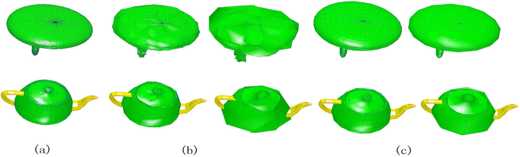
Figure 3. (a) original surfaces perturbed with white noise; (b) the surfaces performed lazy wavelet analysis once and twice; (c) the surfaces performed our scheme once and twice.

Figure 3. (a) original surfaces perturbed with white noise; (b) the surfaces performed lazy wavelet analysis once and twice; (c) the surfaces performed our scheme once and twice.

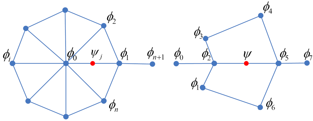
Figure 4. Constructing wavelets as linear combination of lazy wavelets and scaling functions in radial layers.

Figure 4. Constructing wavelets as linear combination of lazy wavelets and scaling functions in radial layers.

Figure 5. Discrete subdivision masks of basis functions in radial layers (lazy wavelets and scaling functions).

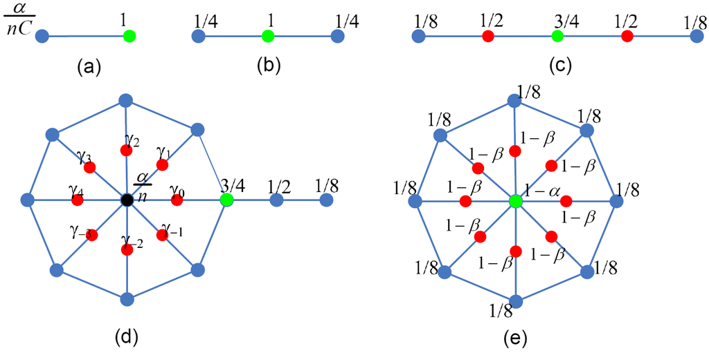
Figure 5. Discrete subdivision masks of basis functions in radial layers (lazy wavelets and scaling functions).

As shown in Figure 6(a), we construct new wavelets ${\psi }_{i,j}^{″}$ by combining the lazy wavelets ${\psi }_{i,j}^{\prime }$ with scaling functions whose corresponding vertices are neighbors to $e_{i,j}^{\prime }$ in circular layers. Since these lifted wavelets should be orthogonalized with the scaling functions, so we need to obtain the weights $w_i$, such that:

$${\psi }_{i,j}^{″}={\psi }_{i,j}^{\prime }+\sum _{k=-2}^3{w}_k{\varphi }_{i,j+k}^{\prime }and\langle {\psi }_{i,j}^{″},{\varphi }_{i,j+k}^{\prime }\rangle =0$$

(7)

Figure 6. (a) Constructing wavelets as linear combination of lazy wavelets and scaling functions in circular layers; (b) Discrete subdivision masks of basis functions in circular layers (lazy wavelets and scaling functions).

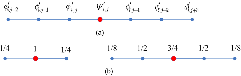
Figure 6. (a) Constructing wavelets as linear combination of lazy wavelets and scaling functions in circular layers; (b) Discrete subdivision masks of basis functions in circular layers (lazy wavelets and scaling functions).

To solve the Equation (7), we need to calculate the inner products of basis functions. A proper inner product could considerably improve the result quality and reduce the complexity of computation. Here we adopt the definition of inner product introduced by Bertram [11]. He suppose the scaling functions of finer resolution form an orthogonal basis without considering all correlation of finer-level coefficients. The mutual inner products of wavelets and scaling functions are defined as the sum of corresponding multiplications of their discrete subdivision masks. This kind of inner product can be calculated directly from the discrete subdivision masks, shown in Figure 6(b), and avoid complex computation needed by the inner product defined with continuous shape of basis functions. More details of local inner production are referred in Bertram’s work. Therefore, without considering the boundary of control nets, we have the inner products of lazy wavelets:

$$\begin{array}{ccc}& \langle {\psi }_{i,j},{\varphi }_{i,j-1}\rangle =\langle {\psi }_{i,j},{\varphi }_{i,j+2}\rangle =1/32\hfill & \hfill \langle {\psi }_{i,j},{\varphi }_{i,j}\rangle =\langle {\psi }_{i,j},{\varphi }_{i,j+1}\rangle =23/32\\ & \langle {\varphi }_{i,j},{\varphi }_{i,j-2}\rangle =\langle {\varphi }_{i,j},{\varphi }_{i,j+2}\rangle =1/64\hfill & \hfill \langle {\varphi }_{i,j},{\varphi }_{i,j-1}\rangle =\langle {\varphi }_{i,j},{\varphi }_{i,j+1}\rangle =7/16\\ & \langle {\varphi }_{i,j},{\varphi }_{i,j}\rangle =35/32\hfill \end{array}$$

Insert the inner products to Equation (7). and we get equation systems:

$$Aw=bwhere{a}_{mn}=\langle {\varphi }_{i,m}^{\prime },{\varphi }_{i,n}^{\prime }\rangle ,b_{mn}=-\langle {\psi }_{i,m}^{\prime },{\varphi }_{i,n}^{\prime }\rangle$$

(8)

After solving these systems, we get weights w which can be precomputed for efficiency.

3.2. Wavelet synthesis and analysis

Suppose $M^i$ is arbitrary circular layer of the surface, we have:

$$M^i=\sum _m{v}_{i,m}^{\prime }{\phi }_{i,m}^{\prime }+\sum _n{e}_{i,n}^{\prime }{\psi }_{i,n}^{\prime }.\forall m,\forall n$$

(9)

By inserting Equation (7) to Equation (9), we get:

$$M^i=\sum _i{v}_{i,m}{\phi }_{i,m}+\sum _j{e}_{i,n}{\psi }_{i,n}+\sum _n{e}_{i,n}(\sum _{k=-1}^2{w}_k{\phi }_{i,n})\forall m,\forall n.$$

(10)

¿From Equation (10), we can construct a new wavelet synthesis from the original lazy wavelets by additional lifting operation prior to the subdivision masks:

$$\begin{array}{cc}& v_{i,j+k}^{\prime }=v_{i,j+k}^{\prime }+w_k{e}_{i,j}^{\prime }\forall k=-2,-1,...,3,\forall i,\hfill \\ & e_{i,j}^{″}=e_{i,j}^{\prime }+\frac{1}{2}(v_{i,j}^{\prime }+v_{i,j+1}^{\prime }),v_{i,j}^{″}=\frac{1}{4}(e_{i,j-1}^{″}+2v_{i,j}^{\prime }+e_{i,j}^{″}).\hfill \end{array}$$

(11)

By inverting the rules of wavelet synthesis process, we can get the new rules for wavelet analysis in circular layers:

$$\begin{array}{cc}& v_{i,j}^{\prime }=\frac{1}{2}(4v_{i,j}^{″}-e_{i,j-1}^{″}-e_{i,j}^{″}),e_{i,j}^{\prime }=e_{i,j}^{″}-\frac{1}{2}(v_{i,j}^{\prime }+v_{i,j+1}^{\prime }),\hfill \\ & v_{i,j+k}^{\prime }=v_{i,j+k}^{″}-w_k{e}_{i,j}^{\prime }\forall k=-2,-1,...,3,\forall i.\hfill \end{array}$$

(12)

The rules of wavelet transforms in radial layer can be obtained by the similar methods. More discussion about the wavelets in radial layers is given in our previous work [20]. Here we only show the wavelet analysis rules in radial layers:

$$\begin{array}{cc}& v=\frac{1}{U}(v^{\prime }-\frac{\alpha }{n\beta }\sum _{k=0}^{n-1}{e}_k^{\prime }),v_j=\frac{8}{5}\times (v_j^{\prime }-\frac{1}{8}v-\frac{1}{4}{e}_{2,j}^{\prime }),\hfill \\ & v_{i,j}=2\times (v_{i,j}^{\prime }-\frac{1}{4}(e_{i-1,j}^{\prime }+e_{i,j}^{\prime }))\forall j,\forall i>1,\hfill \\ & e_j=e_j^{\prime }-(1-\beta )v-\sum _{k=0}^{n-1}{v}_k{\gamma }_{k-j},e_{i,j}=e_{i,j}^{\prime }-\frac{1}{2}(v_{i-1,j}+v_{i,j})\forall j,\forall i>1,\hfill \\ & v_k=v_k-t_k{e}_j\forall j,\forall k=0,...,n-1,\hfill \\ & v_k=v_k-s_k{e}_{i,j}\forall j,\forall i>1,\forall k=0,...,7.\hfill \end{array}$$

(13)

where t and s is the precomputed weights in radial layers, $\alpha =\beta -\frac{1}{4}$, $\beta =\frac{1}{2}$, ${\gamma }_k=\frac{1}{n}(\beta -\frac{1}{2}+\frac{5}{8}{c}_n^k+{(c_n^k)}^2+\frac{1}{2}{(c_n^k)}^3)$, $c_n^k=cos(\frac{2k\pi }{n})$, $U=(1-\alpha )-\frac{\alpha }{\beta }(1-\beta )$. By applying the rules of polar subdivision wavelet transforms, we can give the algorithms of synthesis and analysis. Since the synthesis algorithm is similar to analysis algorithm except the order of sub-steps. Here, we only show the analysis algorithm: For a given polar structure, one step of polar subdivision wavelets analysis includes.

(i)

Performing the wavelet analysis in circular layers. For each circular layer i ($i>0$), we perform:

(a)

lazy wavelet analysising: for each vertex $v_{i,m}$ in circular layer i, denote $v_{i,m}$ (m = 0, 2, 4, 6,...) as the $v_{i,j}^{″}$ (j = m/2), and $v_{i,m}$ (m = 1, 3, 5,...) as $e_{i,j}^{″}$ (j=(m-1)/2). Calculate each $v_{i,j}^{\prime }$ and each $e_{i,j}^{\prime }$ from $v_{i,j}^{″}$ and $e_{i,j}^{″}$ through Equation (6);

(b)

lifting operations on $v_{i,m}^{\prime }$; for each $e_{i,j}^{\prime }$, calculate $v_{i,j+k}^{\prime }$ around $e_{i,j}^{\prime }$ through $v_{i,j+k}^{\prime }=v_{i,j+k}^{\prime }-w_k{e}_{i,j}^{\prime }\forall k=-2,-1,...,3,\forall i$.

(ii)

Performing the wavelet analysis on radial layers based on the results of (i). For each radial layer j, we perform:

(a)

lazy wavelet analysising: for each vertex $v_{m,j}^{\prime }$ in radial layer j, denote $v_{m,j}^{\prime }$ (m = 2, 4, 6,...) as the $v_{i,j}^{\prime }$ (i = m/2), and $v_{m,j}$ (m = 1, 3, 5,...) as $e_{i,j}^{\prime }$ (i = (m-1)/2). Calculate polar vertex v, each $v_{i,j}$ and each $e_{i,j}$ from $v_{i,j}^{\prime }$ and $e_{i,j}^{\prime }$ through Equation (3);

(b)

lifting operations on $v_{i,m}^{\prime }$. for each $e_{i,j}^{\prime }$, calculate $v_{i,j+k}^{\prime }$ around $e_{i,j}^{\prime }$ through $v_k=v_k-t_k{e}_j(\forall j,\forall k=0,...,n-1);v_k=v_k-s_k{e}_{i,j}(\forall j,\forall i>1,\forall k=0,...,7)$.

No matter in radial layers or circular layers, each sub-step of analysis and synthesis must be performed for all points, over the entire mesh before the next sub-step.

4. Bicubic B-spline Subdivision Wavelets

Formally a realistic model may be composed of the polar structures and the quadrilaterals surrounding the polar structures, shown in Figure 1. In fact the polar structures can also be considered as the combination of extraordinary mesh points surrounded by triangles, and quadrilaterals that have points of valence four. The extraordinary mesh points need only be separated by one layer of points of valence four. For the quadrilaterals, we can apply the classical subdivisions, such as Catmull-Clark subdivision. Both Catmull-Clark and polar subdivision generalize bicubic spline subdivision. They can form a powerful combination for smooth object design: while Catmull-Clark subdivision can be applied to the points of valence four, polar subdivision can be applied to the regions surrounding polar vertex. Myles et al. [17] have shown how to combine the meshes of these two generalizations of bicubic B-spline subdivision. Based on their work, we can develop a compound subdivision wavelets on the meshes with quadrilateral faces. Catmull-Clark subdivision wavelet can be applied to the ordinary points while polar subdivision wavelets can be applied on extraordinary points.

The Catmull-Clark subdivision wavelets have been constructed with local lifting by Bertram [9] and Wang et al. [13]. These schemes can be applied directly to the regions of common quadrilaterals(not include the quadrilaterals in polar structures). In Myles’s scheme, the overlap regions between common quadrilaterals and polar structures are both subdivided by Catmull-Clark subdivision and polar subdivision,and drop the boundary facets of the meshes subdivided in polar subdivision and Catmull-Clark subdivision and join them by identifying the resulting boundary vertices. He proved that the jointed subdivision surface is $C^1$ continuity and has bounded curvatures. Because of the different local lifting schemes applied to Catmull-Clark subdivision and polar subdivision, we need make an adjustment to the local lifting schemes in order to keep the continuity of two parts.

The process of wavelet analysis in overlap region is shown in Figure 7. We consider the overlap regions as the extend part of polar structures and adopt the way similar to the construction of polar subdivision wavelets. The stencils for local lifting are shown in Figure 8. By applying this scheme, we can get the decomposition rules in the overlap regions:

$$\begin{array}{cc}& v_{i,j}=\frac{1}{2}(4v_{i,j}^{\prime }-e_{i,j-1}^{\prime }-e_{i,j}^{\prime }),e_{i,j}=e_{i,j}^{\prime }-\frac{1}{2}(v_{i,j-1}+v_{i,j}),\hfill \\ & v_{i,j+k}=v_{i,j+k}-w_k{e}_{i,j}\forall k=-1,0,1,2,\forall i.\hfill \end{array}$$

(14)

and reconstruction rules in the overlap regions:

$$\begin{array}{cc}& v_{i,j+k}=v_{i,j+k}+w_k{e}_{i,j}\forall k=-1,0,1,2,\forall i,\hfill \\ & e_{i,j}^{\prime }=e_{i,j}+\frac{1}{2}(v_{i,j}+v_{i,j+1}),v_{i,j}^{\prime }=\frac{1}{4}(e_{i,j-1}^{\prime }+2v_{i,j}+e_{i,j}^{\prime }).\hfill \end{array}$$

(15)

When performing the wavelet analysis on the model, we should separate the polar structures and the remaining quadrilateral meshes, and perform the wavelet analysis in the overlap region at first. After that we can decompose the polar structures and the rest meshes separately. The wavelet synthesis are processed in the reverse order of analysis.

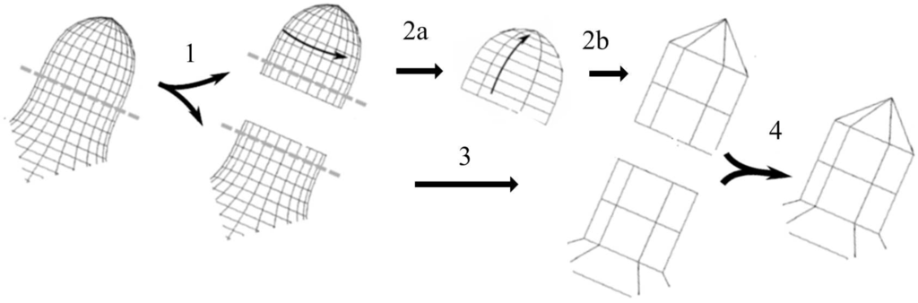
Figure 7. Performing the compound wavelet analysis: (1) separating the input mesh and perform wavelet analysis in the overlap region; (2a) decomposing the polar structure in circular layer; (2b) decomposing the polar structure in radial layer; (3) decomposing the remainder. (4) Joining the resulted meshes after removal of overlapping facets.

Figure 7. Performing the compound wavelet analysis: (1) separating the input mesh and perform wavelet analysis in the overlap region; (2a) decomposing the polar structure in circular layer; (2b) decomposing the polar structure in radial layer; (3) decomposing the remainder. (4) Joining the resulted meshes after removal of overlapping facets.

Figure 8. (a) Constructing wavelets as linear combination of lazy wavelets and scaling functions in radial layers of overlap regions; (b) Constructing wavelets as linear combination of lazy wavelets and scaling functions in circular layers of overlap regions; (c) Discrete subdivision masks of basis functions.

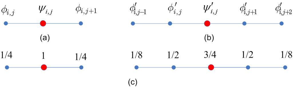
Figure 8. (a) Constructing wavelets as linear combination of lazy wavelets and scaling functions in radial layers of overlap regions; (b) Constructing wavelets as linear combination of lazy wavelets and scaling functions in circular layers of overlap regions; (c) Discrete subdivision masks of basis functions.

5. Experimental Results

Table 1 shows the precomputed weighs $t_i$ and $s_i$ in radial layers when the valence of polar vertex is 8. In radial layers, since the $e_{i,j}$ is far away from the polar vertex when $i>2$, there are no relations between the points in different radial directions. In this situation, $s_1$, $s_3$, $s_4$ and $s_6$ are zero. Table 2 shows the precomputed weighs $w_i$ in circular layers. It can be further improved by combining more scaling functions ${\varphi }_{i,j}^{\prime }$ with ${\psi }_{i,j}^{\prime }$.

Table 1. Precomputed weights in radial layers (n = 8).

$t_i$	$s_i$($v_0=v$)	$s_i$($v_0\in v_j$)	$s_i$ ($v_0\in v_{i,j}$)
-0.212173	0.060810	0.228947	0.189068
-0.239089	0.026201	0.000000	0.000000
-0.052675	-0.560051	-0.544587	-0.525336
0.083197	0.026201	0.000000	0.000000
0.080547	-0.011349	0.000000	0.000000
0.076314	-0.506860	-0.516979	-0.525336
0.080547	-0.011349	0.000000	0.000000
0.083197	0.182173	0.186000	0.189068
-0.052675	-	-	-
0.098667	-	-	-

Table 1. Precomputed weights in radial layers (n = 8).

$t_i$	$s_i$($v_0=v$)	$s_i$($v_0\in v_j$)	$s_i$ ($v_0\in v_{i,j}$)
-0.212173	0.060810	0.228947	0.189068
-0.239089	0.026201	0.000000	0.000000
-0.052675	-0.560051	-0.544587	-0.525336
0.083197	0.026201	0.000000	0.000000
0.080547	-0.011349	0.000000	0.000000
0.076314	-0.506860	-0.516979	-0.525336
0.080547	-0.011349	0.000000	0.000000
0.083197	0.182173	0.186000	0.189068
-0.052675	-	-	-
0.098667	-	-	-

Table 2. Precomputed weights in circular layers.

$w_{-2}$	$w_{-1}$	$w_0$	$w_1$	$w_2$	$w_3$
-0.0829	0.2265	-0.5356	-0.5356	0.2265	-0.0829

Table 2. Precomputed weights in circular layers.

$w_{-2}$	$w_{-1}$	$w_0$	$w_1$	$w_2$	$w_3$
-0.0829	0.2265	-0.5356	-0.5356	0.2265	-0.0829

When performing the multiple levels of wavelet analysis, the stability is an important issue of fitting operations. In order to examine the stability of our polar subdivision based wavelets, we perform a noise-filtering experiment similar to [11, 13, 14]. First, we subdivide the mesh 4 times by polar subdivision, and perturb the subdivided mesh with white noise to all vertices of the final mesh. Then, the perturbed surface will be analyzed step by step by using our wavelet analysis algorithm 4 times. At each resolution, we subdivide the mesh to level 4 (the highest resolution) again without considering the wavelet coefficients of any higher resolution. By this way, we get a sequence of low-pass filtered versions of the noisy mesh, shown in Figure 9. We can compare the difference between low-pass filtered versions of noisy mesh and the original unperturbed mesh by calculating the corresponding $L_2$-norm errors. The test results in Table 3 and Table 4 show that the error does not significantly increase after multiple steps of wavelet analysis operations. In contrast to the lazy wavelets, our wavelet scheme has a good performance of stability. Figure 10 shows the results of compound wavelet analysis. After wavelet analysis, the polar structures and the rest quadrilateral meshes are smoothly joined.

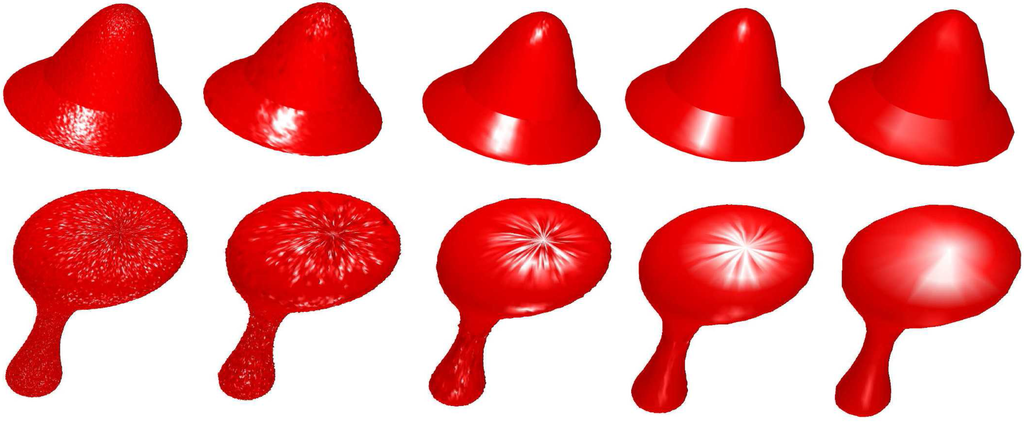
Figure 9. Progressive wavelet analysis of surfaces (with white noises) from level 4 to level 0.

Figure 9. Progressive wavelet analysis of surfaces (with white noises) from level 4 to level 0.

Table 3. $L_2$ error of hat in different levels (with and without lifting).

Level	Number of vertices	$L_2$ error of our scheme (with)	$L_2$ error of lazy wavelets (without)
4	24577	0.00192136	0.00192128
3	6145	0.00096071	0.00475723
2	1537	0.00061625	0.017283
1	385	0.000485615	0.0720949
0	97	0.000562381	0.251045

Table 3. $L_2$ error of hat in different levels (with and without lifting).

Level	Number of vertices	$L_2$ error of our scheme (with)	$L_2$ error of lazy wavelets (without)
4	24577	0.00192136	0.00192128
3	6145	0.00096071	0.00475723
2	1537	0.00061625	0.017283
1	385	0.000485615	0.0720949
0	97	0.000562381	0.251045

Table 4. $L_2$ error of mushroom in different levels (with and without lifting).

Level	Number of vertices	$L_2$ error of our scheme (with)	$L_2$ error of lazy wavelets (without)
4	55297	0.00194545	0.00198193
3	13825	0.000941068	0.00477773
2	3457	0.000538884	0.0179629
1	865	0.000344581	0.0756179
0	217	0.000270338	0.333253

Table 4. $L_2$ error of mushroom in different levels (with and without lifting).

Level	Number of vertices	$L_2$ error of our scheme (with)	$L_2$ error of lazy wavelets (without)
4	55297	0.00194545	0.00198193
3	13825	0.000941068	0.00477773
2	3457	0.000538884	0.0179629
1	865	0.000344581	0.0756179
0	217	0.000270338	0.333253

From the rules of polar subdivision wavelet transforms, we know that the computations of lifting are executed over each vertex. And the time complexity of computation over one vertex is O(1). So the time complexity of lifting operation only depends the number of vertices of polar structures. Since the time complexity of polar subdivision is O(n) (n is the number of vertices of polar structure), the time complexity of the whole wavelet transforms is O(n). Since it is not necessary to use the filter banks (they often mean large matrices) to perform the wavelet transforms and the computation is fully in-place, there is no additional memory cost either. The space complexity of wavelet transforms also depends on the number of vertices of polar structure. The well-designed data structures based on the principle of polar structure can effectively reduce the memory cost further.

Figure 10. Mesh sequences in different resolution: (a) the original meshes; (b) the meshes by wavelet analysis once; (c) the meshes by wavelet analysis twice; (d) the surface of polar structures by wavelet analysis twice.

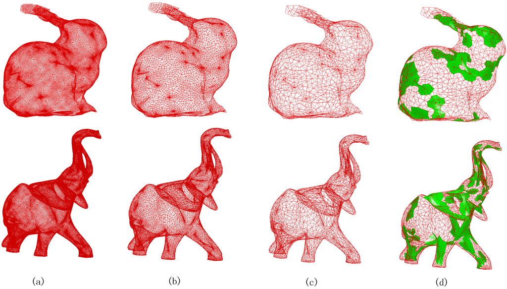
Figure 10. Mesh sequences in different resolution: (a) the original meshes; (b) the meshes by wavelet analysis once; (c) the meshes by wavelet analysis twice; (d) the surface of polar structures by wavelet analysis twice.

Table 5. The test results of performing polar subdivision wavelet transforms in different orders. For simple, we name the resulted meshes by performing analysis in radial layers first as A; the resulted meshes by performing analysis in circular layer first as B; O means original unperturbed meshes. The table lists the $L_2$ error between any two of them.

Mesh	A and B	A and O	B and O
mushroom	0.00001449	0.00200506	0.00200448
hat	0.00018902	0.00577932	0.00577456
hand	0.00017053	0.00491544	0.00491222

Table 5. The test results of performing polar subdivision wavelet transforms in different orders. For simple, we name the resulted meshes by performing analysis in radial layers first as A; the resulted meshes by performing analysis in circular layer first as B; O means original unperturbed meshes. The table lists the $L_2$ error between any two of them.

Mesh	A and B	A and O	B and O
mushroom	0.00001449	0.00200506	0.00200448
hat	0.00018902	0.00577932	0.00577456
hand	0.00017053	0.00491544	0.00491222

Though the subdivisions in radial layers and circular layers are independent, more testing is necessary to determine which should perform first. We performed the experiments on both selective orders. We perturbed the original meshes with white noise, and performed wavelet analysis on the perturbed meshes. Then we subdivided the new meshes to original resolution, and compared them with the original unperturbed ones by calculating $L_2$ errors. From the experimental results shown in Table 5, we find that there is only a small difference between the orders, especially if many vertices in the complex models. Myles et al. [18] provided the revised polar subdivision with the $C^2$ continuity on polar vertices, which synthesized the subdivision rules of radial and circular layers in a more tightly way. As the wavelet framework facilitates both multiresolution analysis and synthesis efficiently, our proposed wavelet scheme inherits the advantages of subdivision and provides the stable shape preservation for analysis, by performing the local lifting operations.

6. Conclusion

In this paper, we proposed the novel compound biorthogonal wavelets for representing quadrilateral meshes with polar structures in multiresolution, based on polar subdivision and Catmull-Clark subdivision. The polar subdivision wavelets are naturally suitable to decompose and reconstruct surfaces of revolution. By using local lifting and orthogonalization, the wavelet analysis and synthesis are fully in-place and can be performed in linear time. As the wavelets are constructed in radial and circular layers, they can be directly combined with other quadrilateral subdivisions, such as Catmull-Clark subdivision. By performing the wavelet analysis in circular layers, we reduce the valence of polar vertex, which is useful in dealing with the meshes with high valence extraordinary vertices. To seamlessly combine with the Catmull-Clark subdivision wavelets, we developed the special operations to construct the wavelets in the circular layers of polar structures. These operations guarantee the continuity of the polar structures and the remaining meshes in different resolutions. Because the orthogonality of wavelet basis functions are improved by local lifting, the computation of our proposed wavelet scheme is highly efficient and fully in-place. Further, we will work on constructing the uniform polar subdivision wavelets, and there is no need to perform the steps in circular and radial layers separately.

References

- Lounsbery, M.; DeRose, T.; Warren, J. Multiresolution analysis for surfaces of arbitrary topological type. ACM Trans. Graph. 1997, 16, 34–73. [Google Scholar] [CrossRef]
- Valette, S.; Prost, R. Wavelet-based multiresolution analysis of irregular surface meshes. IEEE Trans. Visual. Comput. Graph. 2004, 10, 113–122. [Google Scholar] [CrossRef] [PubMed]
- Valette, S.; Prost, R. Wavelet-based progressive compression scheme for triangle meshes: wavemesh. IEEE Trans. Visual. Comput. Graph. 2004, 10, 123–129. [Google Scholar] [CrossRef] [PubMed]
- Samavati, F.F.; Bartels, R.H. Multiresolution curve and surface representation: reversing subdivision rules by least-squares data fitting. Comput. Graph. Forum 1999, 18, 97–119. [Google Scholar] [CrossRef]
- Samavati, F.F.; R.H. Bartels, N. M.-A. Multiresolution surfaces having arbitrary topologies by a reverse Doo subdivision method. Computer Graphics Forum 2002, 21, 121–136. [Google Scholar] [CrossRef]
- Khodakovsky, A.; Schröder, P.; Swelddens, W. Progressive geometry compression. In Proceedings of the 27th annual conference on Computer graphics and interactive techniques, New York, NY, USA, July, 2000; pp. 271–278.
- Sweldens, W. The lifting scheme: A custom-design construction of biorthogonal wavelets. Appl. Comput. Harmon. Anal. 1996, 3, 186–200. [Google Scholar] [CrossRef]
- Schröder, P.; Sweldens, W. Spherical wavelets: efficiently representing functions on the sphere. In Proceedings of the 22nd annual conference on Computer graphics and interactive techniques, New York, NY, USA, 1995; pp. 161–172.
- Bertram, M.; Duchaineau, M.; Hamann, B.; Joy, K. Generalized B-spline subdivision-surface wavelets for geometry compression. IEEE Trans. Visual. Comput. Graph. 2004, 10, 326–338. [Google Scholar] [CrossRef] [PubMed]
- Bertram, M.; Duchaineau, M.; Hamann, B.; Joy, K. Bicubic subdivision-surface wavelets for large-scale isosurface representation and visualization. In Proceedings of the conference on Visualization ’00, Salt Lake City, UT, USA, October 8–13, 2000; pp. 389–396.
- Bertram, M. Biorthogonal loop-subdivision wavelets. Computing 2004, 72, 29–39. [Google Scholar] [CrossRef]
- Li, D.; Qin, K.; Sun, H. Unlifted Loop Subdivision Wavelets. In Proceedings of 12th Pacific Conference on the Computer Graphics and Applications, Seoul, Korea, October 6–8, 2004; 2004; pp. 25–33. [Google Scholar]
- Wang, H.; Qin, K.; Tang, K. Efficient wavelet construction with Catmull-Clark subdivision. Vis. Comput. 2006, 22, 874–884. [Google Scholar] [CrossRef]
- Wang, H.; Qin, K.; Sun, H. -Subdivision-based biorthogonal wavelets. IEEE Trans. Visual. Comput. Graph. 2007, 13, 914–925. [Google Scholar] [CrossRef] [PubMed]
- Karčiauskas, K.; Myles, A.; Peters, J. A C2 polar jet subdivision. In Proceedings of the 4th Eurographics symposium on Geometry processing, Cagliari, Sardinia, Italy, June 26–28, 2006; pp. 173–180.
- Karčiauskas, K.; Peters, J. Bicubic polar subdivision. ACM Trans. Graph. 2007, 26, 1–8. [Google Scholar] [CrossRef]
- Myles, A.; Karciauskas, K.; Peters, J. Extending catmull-clark subdivision and PCCM with polar structures. In Proceedings of the 15th Pacific Conference on Computer Graphics and Applications, Maui, Hawaii, USA, October 29–November 2, 2007; pp. 313–320.
- Myles, A.; Peters, J. Bi-3 C2 polar subdivision. In SIGGRAPH 2009 Papers; ACM: New York, NY, USA, 2009; pp. 1–12. [Google Scholar]
- Khodakovsky, A.; Schroder, P.; Sweldens, W. Progressive geometry compression. In Proceedings of the 27th Annual Conference on Computer Graphics and Interactive Techniques, New York, NY, USA, July, 2000; ACM Press/Addison-Wesley Publishing Co.: New Orleans, LA, USA, 2000; pp. 271–278. [Google Scholar]
- Zhao, C.; Wang, H.; Sun, H.; Qin, K. Polar subdivision based wavelet analysis. In Proceedings of the 2008 International Conference on Computer Graphics and Virtual Reality (Computer Graphics International 2008), Las Vegas, NV, USA, July 14–17, 2008. CDROM.
© 2009 by the authors; licensee Molecular Diversity Preservation International, Basel, Switzerland. This article is an open-access article distributed under the terms and conditions of the Creative Commons Attribution license http://creativecommons.org/licenses/by/3.0/.