Abstract
Functional connectivity (FC) studies have demonstrated the overarching value of studying the brain and its disorders through the undirected weighted graph of functional magnetic resonance imaging (fMRI) correlation matrix. However, most of the work with the FC depends on the way the connectivity is computed, and it further depends on the manual post-hoc analysis of the FC matrices. In this work, we propose a deep learning architecture BrainGNN that learns the connectivity structure as part of learning to classify subjects. It simultaneously applies a graphical neural network to this learned graph and learns to select a sparse subset of brain regions important to the prediction task. We demonstrate that the model’s state-of-the-art classification performance on a schizophrenia fMRI dataset and demonstrate how introspection leads to disorder relevant findings. The graphs that are learned by the model exhibit strong class discrimination and the sparse subset of relevant regions are consistent with the schizophrenia literature.
1. Introduction
Functional connectivity, which is often computed using cross-correlation among brain regions of interest (ROIs), is a powerful approach that has been shown to be informative for classifying brain disorders and revealing putative bio-markers that are relevant to the underlying disorder [1,2,3,4]. Inferring and using functional connectivity through spatio-temporal data, e.g., functional magnetic resonance imaging (fMRI), has been an especially important area of research in recent times. Functional connectivity can improve our understanding of brain dynamics and improve classification accuracy for brain disorders, such as schizophrenia. Recent work [5] uses functional network connectivity (FNC) as features to predict schizophrenia related changes. Whereas, Parisot et al. [6] uses functional connectivity obtained by a fixed formula with phenotypic and imaging data as inputs and to extract graphic features for the classification of AD and Autism. Kawahara et al. [7] also uses the connection strength between brain regions as edges, being typically defined as the number of white-matter tracts connecting the regions. Ktena et al. [8] employs spectral graph theory to learn similarity metrics among the functional connectivity networks.
These papers, as well as many others, have shown the efficacy of functional connectivity and feature extraction based on neural network models. However, existing studies often heavily depend on the underlying method of functional connectivity estimation, in terms of classification accuracy, feature extraction, or learning brain dynamics. Studies, like [9,10,11], depend on hand-crafted features based on methods, like ICA (Independent Component Analysis). These studies work very well on classification, but they do not learn a sparse graph and are not helpful in identifying bio-markers in the brain.
Many functional connectivity studies [12] on brain disorders utilize ROIs predefined based on anatomical or functional atlases, which are either fixed for all subjects or based on group differences.
These approaches ignore the possibility of inter-subject variations of ROIs, especially the variations due to the underlying disease conditions. They also rely on the complete set of these ROIs discounting the possibility that only a small subset may be important at a time. A disorder can have varying symptoms for different people, hence making it crucial to determine disorder and subject specific ROIs.
In this work, we address the problems of using a fixed method of learning functional connectivity and using it as a fixed graph to represent brain structure (the standard practices) by utilizing a novel attention based Graph Neural Network (GNN) [13], which we call BrainGNN. We apply it to fMRI data and (1) achieve comparable classification accuracy to existing algorithms, (2) learn dynamic graph functional connectivity, and (3) increase the model interpretability by learning which regions from the set of ROIs are relevant for the classification, enabling additional insights into the health and disordered brain.
2. Materials and Methods
2.1. Materials
In this study, we worked with the data from Function Biomedical Informatics Research Network (FBIRN) (These data were downloaded from Function BIRN Data Repository, Project Accession Number 2007-BDR-6UHZ1.) [14] dataset, including schizophrenia (SZ) patients and healthy controls (HC), for testing our model. Details of the dataset are shown in the following section.
2.1.1. Fbirn
The resting fMRI data from the phase III FBIRN were analyzed for this project. The dataset has 368 total subjects, out of which 311 were selected based on the preprocessing method explained in Section 2.1.2.
2.1.2. Preprocessing
The fMRI data were preprocessed using statistical parametric mapping (SPM12, http://www.fil.ion.ucl.ac.uk/spm/, accessed on 22 February 2021) under the MATLAB 2019 environment. A rigid body motion correction was performed to correct subject head motion, followed by the slice-timing correction to account for timing difference in slice acquisition. The fMRI data were subsequently warped into the standard Montreal Neurological Institute (MNI) space while using an echo planar imaging (EPI) template and they were slightly resampled to mm isotropic voxels. The resampled fMRI images were then smoothed using a Gaussian kernel with a full width at half maximum (FWHM) = 6 mm. After the smoothing, the functional images were temporally filtered by a finite impulse response (FIR) bandpass filter (0.01 Hz–0.15 Hz). Subsequently, for each voxel, six rigid body head motion parameters, white matter (WM) signals and cerebrospinal fluid (CSF) signals, were regressed out using linear regression.
We selected subjects for further analysis [15] if the subjects have head motion ≤ and ≤3 mm, and with functional data providing near full brain successful normalization [16].
This resulted in a total of 311 subjects with 151 healthy controls and 160 subjects with schizophrenia. Each subject is represented by , where represent the number of voxels in each dimension and is the number of time points that are 160. In order to reduce the affect of noise, we zscore the time sequence of each voxel independently. Thus, time series of every voxel is replaced by the z-score of the time series. This does not have any effect on the data dimensions.
To partition the data into regions, automated anatomical labeling (AAL) is used [17], which contains 116 brain regions. Taking sum of the voxels inside a region is an easy and common method, but this gives an unfair advantage to bigger regions. For this, we take the weighted average of the voxel intensities inside a region. Weight is the value of a voxel being inside a region, as these values are not binary. Averaging helps to negate the bias towards bigger regions. This results in a dataset , where , , , .
2.2. Method
We have three distinct parts in our novel attention based GNN architecture: (1) a Convolutional Neural Network (CNN) [18] that creates embeddings for each region, (2) a Self-Attention mechanism [19] that assigns weights between regions for functional connectivity, and (3) a GNN that uses regions (nodes) and edges for graph classification. In this section, we separately explain the purpose and details of each part. Refer to Figure 1 for the complete architecture diagram of BrainGNN.
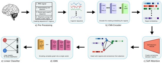
Figure 1.
BrainGNN architecture using: (a) Preprocessing: to preprocess the raw data with different steps (Section 2.1.2); (b) 1DCNN: to create embedding for regions (Section 2.2.1); (c) Self-attention: to create connectivity between regions (Section 2.2.2); (d) GNN: to obtain a single feature vector for the entire graph (Section 2.2.3); and (e) Linear classifier: to obtain the final classification.
2.2.1. Cnn Encoder
We use a CNN [20] encoder to obtain the representation of individual regions created in the preprocessing step that is outlined in Section 2.1.2. Each region vector of dimension is passed through multiple layers of one dimensional convolution, and a fully connected layer to obtain final embedding. The one dimensional CNN encoder used in our architecture consists of 4 convolution layers with filter size , stride and output channels . This is followed by a fully connected layer that results in a final embedding of size 64. We use the rectified linear unit (ReLU) as an activation layer between convolution layers. Each region is individually encoded to later on create connections between regions and interpret which regions are more important/informative for classification. Our one dimensional CNN layer embeds the temporal features of regions and the spatial connections are handled in the attention and GNN parts of the architecture.
2.2.2. Self Attention
Using the embeddings created by the CNN encoder, we estimate the connectivity between the regions of the brain using multi-head self-attention following [19]. The self-attention model creates three embeddings namely (key, query, value) for each region, which, in our architecture, are created using three simple linear layers. Each linear layer is of size 24. , , and . To create weights between a region and every other region, the model takes the dot product of a region’s query with every other region’s key embedding to obtain scores between them. Hence, . The scores are then converted to weights using softmax. , where is a vector of scores between region i and every other region. The weights are then multiplied with the embedding of each region and summed together to create new representation for a . The following equations show how to get new region embedding and weight values.
This process is carried out for all of the regions, producing a new representation of every region and the weights between regions. These weights are then used as the functional connectivity between different regions of brain for every subject. The self attention layer encodes the spatial axis for each subject and provides the connection between regions. The weights are learned via end-to-end learning of our model performing classification. This frees us from using predefined models or functions to estimate the connectivity.
2.2.3. GNN
Our graph network is based on a previously published model [13]. Each subject is represented by a graph G having , where is the matrix of vertices, where each vertex is represented by an embedding acquired by self-attention. are the adjacency and edge weight matrices. Because we do not use any existing method of computing edges, we construct a complete directed graph with backward edges, meaning that every pair of vertices is joined by two directed edges with weights and . For each GNN layer, at every step s, each node, which is a region in our model, sums the feature vectors of every other region relative to the weight edge between the nodes and passes the resultant and its own feature vector through a gated recurrent unit (GRU) network [21] to obtain new embedding for itself.
where GRU can be explained by following set of equations, with representing the result of sum in Equation (2):
The number of steps is a hyper-parameter that we have set it as 2 based on our experiments. The graph neural network helps nodes to create new embeddings based on the embeddings of other regions in the graph weighted by the edge weights between them. In our architecture, we use 6 GNN layers, as shown in experiments of [22], which it provides with the highest accuracy, with the first 3, followed by a top-k pooling layer [23,24]. On the input feature vectors, which are the embeddings of the regions, the pooling operator learns a parameter (), which is to assign weight to the features. Based on this parameter, the top (k) layers are chosen in each pooling layer and the rest of the regions are discarded from further layers. The pooling method can be explained by the following equations.
and are the new features and adjacency matrix that we get after selecting top (k) regions. Pooling is performed to help model focus on the important regions/nodes that are responsible for classification. The ratio of nodes to keep in the pooling layer is a hyper-parameter and we have used as the ratios. Because we represent each subject as graph G, in the end we do graph classification by pooling all the feature vectors of the remaining 23 regions/nodes. To obtain one feature vector from the entire graph, we concatenate the output of three different pooling layers. We pass the complete graph into three separate pooling layers. Each of the pooling layer gives us one feature factor. In the end, we concatenate the three vectors to get one final embedding for the entire graph that represents a subject. In our model, we use graph max pool, graph average pool, and attention based pool [25]. The dimension of the resulting vector is 96. The feature vector is then passed through two linear layers of size 32 and 2. As the name suggests, graph max pool and graph average pool just gets the max and average vector from the graph, whereas attention based pooling multiplies each vector with a learned attention value before summing all of the vectors.
2.2.4. Training and Testing
To train, validate, and test our model, we divide the total 311 subjects into three groups of size 215, 80, and 16, for training, validating, and testing, respectively. To conduct a fair experiment, we use 19 fold cross validation and, for each fold, we perform 10 trials, resulting in a total of 190 trials, and selecting 100 subjects per class for each trial. We calculate the area under the ROC (receiver operating characteristic) curve (AUC) for each trial. To optimize our model, we train all of our architecture in an end to end fashion, using Cross Entropy to calculate our loss by giving true labels Y as targets, Adam as our optimizer, and reducing learning rate on a plateau with a patience of 10. We early stop our model based on validation loss, with a patience of 15. Let represent the parameters of the entire architecture.
3. Results
We show three different groups of results in our study. (1) The classification results; (2) regions’ connectivity; and (3) key regions selection. We discuss these in the following sections. We test and compare our model against the classical machine learning algorithms and [26] on the same data used in BrainGNN. The input for the machine learning model is sFNC matrices that are produced using Pearson product-moment correlation coefficients (PCC).
3.1. Classification
As mentioned, we use the AUC metric to quantify the classification results of our model. AUC is more informative than simple accuracy for binary classification, as in our case. Figure 2 shows the results for our model. Figure 3 shows the ROC curves of the models for each fold. The performance is comparable to state of the art classical machine learning algorithms using hand crafted features and existing deep learning approaches, such as [26], which performed the test on independent component analysis (ICA) components with a hold out dataset. Figure 4 presents a comparison with other machine and deep learning approaches and it proves our claim of BrainGNN providing state of the art results. BrainGNN gives almost the same mean AUC as the best performing model, i.e., SVM (Support Vector Machine). To the best of our knowledge, these results are currently among the best on the unmodified FBIRN fMRI dataset [9,10,11]. Table 1 shows the mean AUC for each cross validation fold that was used for experimentation for BrainGNN. The AUC has high variance across the different test sets of cross validation, as it is shown in the table. To make more sense out of the functional connectivity and region selection, both of the results are based on the second test fold, which gives the highest (∼1) AUC score.
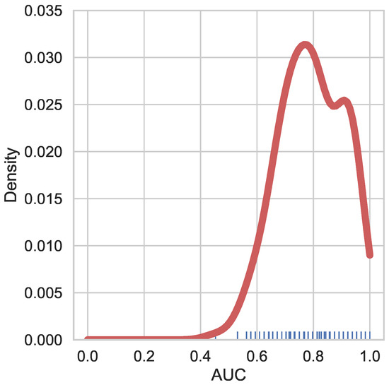
Figure 2.
KDE plot of probability density of receiver operating characteristic curve (ROC-AUC) score on Function Biomedical Informatics Research Network (FBIRN) dataset. The 190 points on the x-axis signifies the 19 fold cross validation, 10 trials per cross validation. With average and median of (∼0.8), density peaks at (∼0.8) AUC.
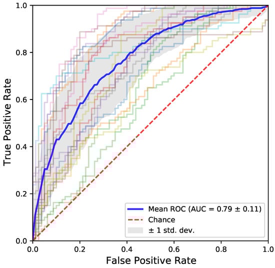
Figure 3.
The ROC curves of the 19 models generated using each fold of cross validation. The graph is symmetrical and well balanced. It shows that the model did not learn one class over the other.
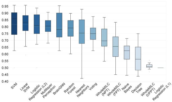
Figure 4.
BrainGNN comparision with other popular methods. BrainGNN provides mean AUC as , which is just (∼0.02) less than the best performing model (SVM). Methods like WholeMILC (UFPT) and l1 logistic regression failed to learn on the input data. The l1 logistic regression model does perform better with a very weak regularization term.

Table 1.
Showing mean AUC of 10 trials for each cv fold.
3.2. Functional Connectivity
The functional connectivity between regions of the brain is crucial in understanding how different parts of brain interact with each other. We use the weights that are assigned by the self-attention module of our architecture as the connection between regions. Figure 5 shows the weight matrices for the second test set in cross validation. Weight matrices of subjects belonging to SZ class turn out to be much sparser than weights of healthy controls subjects. The result shows that the connectivity is limited to fewer regions, and the functional connectivity differs across classes and fewer regions get higher weights in the case of SZ subjects. We also perform statistical testing to confirm that the weight matrices of HC differ from those of the SZ subjects. We create two sets, each representing the concatenation of the weights of 8 test subjects that belong to a class. We perform 2 different testing, as shown in Table 2. A p-value of < shows that we can reject the null-hypothesis, hence making it highly likely that the difference between the weights of HC and SZ subjects is not zero. FNC matrices that are produced using the PCC method do not provide such a level of information and almost all regions get unit weight between other regions. Figure 5 shows the usefulness of learning connectivity between regions in an end-to-end manner while training the model for classification.
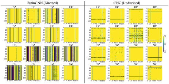
Figure 5.
Connectivity between regions of subjects of both classes using BrainGNN and sFNC (PCC method). BrainGNN: the similarity of connection between a class and difference across class is compelling. Weights of SZ class are more sparse than HC, highlighting the fact that fewer regions receive higher weights for subjects with SZ. Refer to Table 2 for results of statistical testing between weights of HC and SZ subjects. sFNC: the matrices are symmetric but are less informative than those that were produced by BrainGNN. Most of the regions are assigend unit weight.
Table 2.
Statistical testing between weight matrices of healthy controls (HC) and schizophrenia (SZ). The test shows that weights of regions differ across HC and SZ subjects. Refer to Figure 4 for mean and deviation of these folds.
3.3. Region Selection
The pooling layer added in our GNN module allows for us to reduce the number of regions. Functionality across brain regions differs significantly and not all regions are affected by a disorder or have any noticeable affect on classification. This makes it very important to know which regions are more significantly informative of the underlying disorder and study how they get affected or affect the disorder. Figure 6a shows the final 23 regions that were selected after the last pooling layer in the GNN model, which is just 20 percent of the total brain regions used. The relevance of these regions is further signified by the fact that the graph model has no residual connections and the final feature vector created after the last GNN layer is through the feature vectors of these regions. Figure 6b shows the location of the selected regions in the MNI brain space, regions are distinguished by color. Each region is assigned one unit from the color bar, which is used to represent signal variation in the fMRI data.
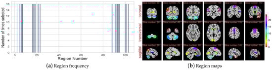
Figure 6.
(a) Histogram of regions selected after the last pooling layer of GNN. 2nd fold of the cross validation gives this figure. All the 23 regions are selected an equal number of times (16). It further signifies the important of these regions, showing that, for all subjects across both classes, these 23 regions are always selection. (b) mapping the 23 regions back on the brain across the three anatomical planes. 100th time point is selected for these brain scans. X axis shows different slices of the plane.
4. Discussion
The richness of results in the three presented categories highlights the benefits of the proposed method. High classification performance shows that the model can accurately classify the subjects and, hence, it can be trusted with the other two interpretative results of the paper. Functional connectivity between the regions shown in the paper is of paramount importance, as it highlights how brain regions are connected to each other and the variation between classes. Learning functional connectivity end-to-end through classification training frees the model from depending on an external method. The sparse weight matrix of subjects with SZ shows that connectivity remains significant between considerably fewer regions than for healthy controls. Notably, the attention based functional connectivity cannot be interpreted as the conventional correlation based symmetric connectivity. Because of the inherent asymmetry in keys and values, the obtained graph is directed, but it is also prediction based rather than simply correlation. We expect that a further investigation into the obtained graph structure will bring more results and deeper interpretations. The sparsity is to be further explored and seen in the context of the regions selected, as shown in the last section of results. The final regions selected by the model strengthens our hypotheses that not all regions are equally important for identifying a particular brain disorder. Reducing the brain regions by almost helps in identifying the important regions for the classification of SZ. The regions selected by our model, such as cerebellum, temporal lobe, caudate, SMA, etc., have been linked to the disease by multiple previous studies, hence reassuring the correctness of our model [27,28,29,30]. We see an immediate benefit of using GNNs to study functional connectivity and our BrainGNN model specifically. The data-driven model almost eliminates manual decisions transitioning graph construction and region selection into the data-driven realm. With this BrainGNN opens up a new direction to the existing studies of connectivity, and we expect further model introspection to yield insight into the spatio-temporal biomarkers of schizophrenia. Further reducing the selected regions and how they different across subjects belonging to different class is also left for future work. We envision great benefits to the interpretability and elimination of manual processing and decisions in a future extension of the model that would enable it to work directly from the voxel-level, not only connecting and selecting ROIs, but also constructing them.
Author Contributions
Conceptualization, U.M., S.P.; methodology, U.M.; software, U.M.; validation, U.M.; formal analysis, U.M.; investigation, U.M.; resources, V.D.C.; data curation, Z.F., U.M.; writing—original draft preparation, U.M.; writing—review and editing, U.M., S.P., Z.F.; visualization, U.M.; supervision, S.P.; project administration, S.P., V.D.C.; funding acquisition, S.P., V.D.C. All authors have read and agreed to the published version of the manuscript.
Funding
This study was in part supported by NIH grants 2RF1MH121885, 1R01AG063153, and 2R01EB006841.
Data Availability Statement
Not Applicable, the study does not report any data.
Acknowledgments
Data for Schizophrenia classification was used in this study were downloaded from the Function BIRN Data Repository (http://bdr.birncommunity.org:8080/BDR/, accessed on 22 February 2021), supported by grants to the Function BIRN (U24-RR021992) Testbed funded by the National Center for Research Resources at the National Institutes of Health, U.S.A. and from the COllaborative Informatics and Neuroimaging Suite Data Exchange tool (COINS; http://coins.trendscenter.org, accessed on 22 February 2021) and data collection was performed at the Mind Research Network, and funded by a Center of Biomedical Research Excellence (COBRE) grant 5P20RR021938/P20GM103472 from the NIH to Vince Calhoun.
Conflicts of Interest
The authors declare no conflict of interest.
References
- Liu, Y.; Liang, M.; Zhou, Y.; He, Y.; Hao, Y.; Song, M.; Yu, C.; Liu, H.; Liu, Z.; Jiang, T. Disrupted small-world networks in schizophrenia. Brain 2008, 131, 945–961. [Google Scholar] [CrossRef]
- Lynall, M.E.; Bassett, D.S.; Kerwin, R.; McKenna, P.J.; Kitzbichler, M.; Muller, U.; Bullmore, E. Functional Connectivity and Brain Networks in Schizophrenia. J. Neurosci. 2010, 30, 9477–9487. [Google Scholar] [CrossRef]
- Yu, R.; Zhang, H.; An, L.; Chen, X.; Wei, Z.; Shen, D. Connectivity strength-weighted sparse group representation-based brain network construction for MCI classification. Hum. Brain Mapp. 2017, 38, 2370–2383. [Google Scholar] [CrossRef]
- Gadgil, S.; Zhao, Q.; Pfefferbaum, A.; Sullivan, E.V.; Adeli, E.; Pohl, K.M. Spatio-Temporal Graph Convolution for Resting-State fMRI Analysis. In Medical Image Computing and Computer Assisted Intervention—MICCAI 2020; Martel, A.L., Abolmaesumi, P., Stoyanov, D., Mateus, D., Zuluaga, M.A., Zhou, S.K., Racoceanu, D., Joskowicz, L., Eds.; Springer International Publishing: Cham, Switzerland, 2020; pp. 528–538. [Google Scholar] [CrossRef]
- Yan, W.; Plis, S.; Calhoun, V.D.; Liu, S.; Jiang, R.; Jiang, T.Z.; Sui, J. Discriminating schizophrenia from normal controls using resting state functional network connectivity: A deep neural network and layer-wise relevance propagation method. In Proceedings of the 2017 IEEE 27th International Workshop on Machine Learning for Signal Processing (MLSP), Tokyo, Japan, 25–28 September 2017; pp. 1–6. [Google Scholar] [CrossRef]
- Parisot, S.; Ktena, S.I.; Ferrante, E.; Lee, M.; Guerrero, R.; Glocker, B.; Rueckert, D. Disease prediction using graph convolutional networks: Application to Autism Spectrum Disorder and Alzheimer’s disease. Med. Image Anal. 2018, 48, 117–130. [Google Scholar] [CrossRef] [PubMed]
- Kawahara, J.; Brown, C.; Miller, S.; Booth, B.; Chau, V.; Grunau, R.; Zwicker, J.; Hamarneh, G. BrainNetCNN: Convolutional Neural Networks for Brain Networks; Towards Predicting Neurodevelopment. NeuroImage 2016, 146. [Google Scholar] [CrossRef]
- Ktena, S.I.; Parisot, S.; Ferrante, E.; Rajchl, M.; Lee, M.; Glocker, B.; Rueckert, D. Distance Metric Learning Using Graph Convolutional Networks: Application to Functional Brain Networks. In Medical Image Computing and Computer Assisted Intervention—MICCAI 2017; Descoteaux, M., Maier-Hein, L., Franz, A., Jannin, P., Collins, D.L., Duchesne, S., Eds.; Springer International Publishing: Cham, Switzerland, 2017; pp. 469–477. [Google Scholar] [CrossRef]
- Rashid, B.; Arbabshirani, M.R.; Damaraju, E.; Cetin, M.S.; Miller, R.; Pearlson, G.D.; Calhoun, V.D. Classification of schizophrenia and bipolar patients using static and dynamic resting-state fMRI brain connectivity. NeuroImage 2016, 134, 645–657. [Google Scholar] [CrossRef]
- Saha, D.K.; Damaraju, E.; Rashid, B.; Abrol, A.; Plis, S.M.; Calhoun, V.D. A classification-based approach to estimate the number of resting fMRI dynamic functional connectivity states. bioRxiv 2020. [Google Scholar] [CrossRef]
- Salman, M.S.; Du, Y.; Lin, D.; Fu, Z.; Fedorov, A.; Damaraju, E.; Sui, J.; Chen, J.; Mayer, A.R.; Posse, S.; et al. Group ICA for identifying biomarkers in schizophrenia: ‘Adaptive’ networks via spatially constrained ICA show more sensitivity to group differences than spatio-temporal regression. NeuroImage 2019, 22, 101747. [Google Scholar] [CrossRef]
- Du, Y.; Fu, Z.; Calhoun, V.D. Classification and Prediction of Brain Disorders Using Functional Connectivity: Promising but Challenging. Front. Neurosci. 2018, 12, 525. [Google Scholar] [CrossRef]
- Li, Y.; Zemel, R.; Brockschmidt, M.; Tarlow, D. Gated Graph Sequence Neural Networks. In Proceedings of the ICLR’16, San Juan, Puerto Rico, 2–4 May 2016. [Google Scholar]
- Keator, D.B.; van Erp, T.G.; Turner, J.A.; Glover, G.H.; Mueller, B.A.; Liu, T.T.; Voyvodic, J.T.; Rasmussen, J.; Calhoun, V.D.; Lee, H.J.; et al. The function biomedical informatics research network data repository. Neuroimage 2016, 124, 1074–1079. [Google Scholar] [CrossRef]
- Fu, Z.; Iraji, A.; Turner, J.A.; Sui, J.; Miller, R.; Pearlson, G.D.; Calhoun, V.D. Dynamic state with covarying brain activity-connectivity: On the pathophysiology of schizophrenia. NeuroImage 2021, 224, 117385. [Google Scholar] [CrossRef]
- Fu, Z.; Caprihan, A.; Chen, J.; Du, Y.; Adair, J.C.; Sui, J.; Rosenberg, G.A.; Calhoun, V.D. Altered static and dynamic functional network connectivity in Alzheimer’s disease and subcortical ischemic vascular disease: Shared and specific brain connectivity abnormalities. Hum. Brain Mapp. 2019. [Google Scholar] [CrossRef] [PubMed]
- Tzourio-Mazoyer, N.; Landeau, B.; Papathanassiou, D.; Crivello, F.; Etard, O.; Delcroix, N.; Mazoyer, B.; Joliot, M. Automated Anatomical Labeling of Activations in SPM Using a Macroscopic Anatomical Parcellation of the MNI MRI Single-Subject Brain. NeuroImage 2002, 15, 273–289. [Google Scholar] [CrossRef]
- Lecun, Y.; Bottou, L.; Bengio, Y.; Haffner, P. Gradient-based learning applied to document recognition. Proc. IEEE 1998, 86, 2278–2324. [Google Scholar] [CrossRef]
- Vaswani, A.; Shazeer, N.; Parmar, N.; Uszkoreit, J.; Jones, L.; Gomez, A.N.; Kaiser, U.; Polosukhin, I. Attention is All You Need. In Proceedings of the 31st International Conference on Neural Information Processing Systems, Long Beach, CA, USA, 4–9 December 2017; pp. 6000–6010. [Google Scholar]
- Kiranyaz, S.; Avci, O.; Abdeljaber, O.; Ince, T.; Gabbouj, M.; Inman, D.J. 1D convolutional neural networks and applications: A survey. Mech. Syst. Signal Process. 2021, 151, 107398. [Google Scholar] [CrossRef]
- Cho, K.; van Merriënboer, B.; Bahdanau, D.; Bengio, Y. On the Properties of Neural Machine Translation: Encoder–Decoder Approaches. In Proceedings of the SSST-8, Eighth Workshop on Syntax, Semantics and Structure in Statistical Translation, Doha, Qatar, 25 October 2014; pp. 103–111. [Google Scholar] [CrossRef]
- Bresson, X.; Laurent, T. Residual Gated Graph ConvNets. arXiv 2017, arXiv:1711.07553. [Google Scholar]
- Gao, H.; Ji, S. Graph U-Nets. arXiv 2019, arXiv:1905.05178. [Google Scholar]
- Knyazev, B.; Taylor, G.W.; Amer, M.R. Understanding Attention and Generalization in Graph Neural Networks. arXiv 2019, arXiv:1905.02850. [Google Scholar]
- Vinyals, O.; Bengio, S.; Kudlur, M. Order Matters: Sequence to sequence for sets. arXiv 2016, arXiv:1511.06391. [Google Scholar]
- Mahmood, U.; Rahman, M.M.; Fedorov, A.; Lewis, N.; Fu, Z.; Calhoun, V.D.; Plis, S.M. Whole MILC: Generalizing Learned Dynamics Across Tasks, Datasets, and Populations. In Medical Image Computing and Computer Assisted Intervention—MICCAI 2020; Martel, A.L., Abolmaesumi, P., Stoyanov, D., Mateus, D., Zuluaga, M.A., Zhou, S.K., Racoceanu, D., Joskowicz, L., Eds.; Springer International Publishing: Cham, Switzerland, 2020; pp. 407–417. [Google Scholar] [CrossRef]
- Jones, D.; Vemuri, P.; Murphy, M.; Gunter, J.; Senjem, M.; Machulda, M.; Przybelski, S.; Gregg, B.; Kantarci, K.; Knopman, D.; et al. Non-Stationarity in the “Resting Brain’s” Modular Architecture. PLoS ONE 2012, 7, e39731. [Google Scholar] [CrossRef]
- Fu, Z.; Sui, J.; Turner, J.A.; Du, Y.; Assaf, M.; Pearlson, G.D.; Calhoun, V.D. Dynamic functional network reconfiguration underlying the pathophysiology of schizophrenia and autism spectrum disorder. Hum. Brain Mapp. 2021, 42, 80–94. [Google Scholar] [CrossRef]
- Ebdrup, B.; Glenthøj, B.; Rasmussen, H.; Aggernaes, B.; Langkilde, A.; Paulson, O.; Lublin, H.; Skimminge, A.; Baaré, W. Hippocampal and caudate volume reductions in antipsychotic-naive first-episode schizophrenia. J. Psychiatry Neurosci. 2010, 35, 95–104. [Google Scholar] [CrossRef]
- Andreasen, N.; Pierson, R. The Role of the Cerebellum in Schizophrenia. Biol. Psychiatry 2008, 64, 81–88. [Google Scholar] [CrossRef] [PubMed]
Publisher’s Note: MDPI stays neutral with regard to jurisdictional claims in published maps and institutional affiliations. |
© 2021 by the authors. Licensee MDPI, Basel, Switzerland. This article is an open access article distributed under the terms and conditions of the Creative Commons Attribution (CC BY) license (http://creativecommons.org/licenses/by/4.0/).