New Bipartite Graph Techniques for Irregular Data Redistribution Scheduling


1
Department of Electronic Engineering, Zhejiang Industry and Trade Vocational College, East Road 717, Wenzhou 325003, China
2
Department of Computer Science and Information Engineering, Chung Hua University, No.707, Sec.2, WuFu Road, Hsinchu 30012, Taiwan
*
Author to whom correspondence should be addressed.
Algorithms 2019, 12(7), 142; https://doi.org/10.3390/a12070142
Submission received: 26 May 2019
/
Revised: 10 July 2019
/
Accepted: 14 July 2019
/
Published: 16 July 2019
Abstract
:For many parallel and distributed systems, automatic data redistribution improves its locality and increases system performance for various computer problems and applications. In general, an array can be distributed to multiple processing systems by using regular or irregular distributions. Some data distribution adopts BLOCK, CYCLIC, or BLOCK-CYCLIC to specify data array decomposition and distribution. On the other hand, irregular distributions specify a different-size data array distribution according to user-defined commands or procedures. In this work, we propose three bipartite graph problems, including the “maximum edge coloring problem”, the “maximum degree edge coloring problem”, and the “cost-sharing maximum edge coloring problem” to formulate these kinds of distribution problems. Next, we propose an approximation algorithm with a ratio bound of two for the maximum edge coloring problem when the input graph is biplanar. Moreover, we also prove that the “cost-sharing maximum edge coloring problem” is an NP-complete problem even when the input graph is biplanar.
1. Introduction
For many years, parallel and distributed networked computer systems have been developed and implemented to tackle compound scientific problems powerfully. Many parallel and distributed systems have been designed to change the distribution of an array at run-time to improve the desired performance. At that time, each processor needs to know which local elements of the array should be sent to the specified processor, and which elements of the array should be received from the specified processor. In general, an array can be distributed to multiple processing systems by using regular or irregular distributions. The former is used in the SCALAPACK library, which uses the block-cyclic data distribution on a virtual grid of processors to reach load-balance on arrays, and adopts equal memory usage between processors [1,2]. On the other hand, an irregular distribution does not adopt specific rules or methods to represent the desired decomposition. Instead, they usually represent the irregular array distribution with the help of user-defined command or procedures. As an example, High Performance Fortran version 2 (HPF2) supports a generalized block distribution (named GEN_BLOCK) format [3,4], when unevenly sized data of an array is to be allocated to a set of processors.
For example, a regular data redistribution using Block-Cyclic(α) to Block-Cyclic(β) (from P processors to Q processors) (denoted by BC(α, β, P, Q)) can be modeled by a bipartite graph GBC(α, β, P, Q) = (X, Y, E), where X = {x0, x1, …, x|X|−1} and Y = {y0, y1, …, y|Y|−1} represent source processor set {p0, p1, …, p|X|−1} and destination processor set {p0, p1, …, p|Y|−1}, respectively. In GBC (α, β, P, Q), if the source processor pi wants to send c elements of the array to the destination processor pj, we add an edge (xi, yj) to E with a weight c. For simplicity, in this work, a shorter symbol BC(α, β, P) is used to represent BC(α, β, P, P).
In Figure 1, a data redistribution pattern BC(1, 4, 4) is depicted as an example, and its weighted distribution graph GBC (1, 4, 4) is also shown in Figure 2. In Figure 1, array elements A(1:16) mapped onto four processors (P) are to be redistributed to four (P) processors. In source distribution, every block with α(=1) element are mapped onto one of processors which are ordered in the cyclic sequence. As a result, A(1), A(5), A(9), A(13) are mapped onto processor P0 in Figure 1. On the other hand, in target distribution, every block with β(=4) element are mapped onto one of the processors which are ordered in the cyclic sequence. Consequently, A(1), A(2), A(3), A(4) are mapped onto processor Q0 in the new distribution. Since A(1), A(2), A(3), A(4) are sent to Q0 by P0, P1, P2, P3, respectively, there are four edges connecting P0, P1, P2, P3 to Q0 in the distribution graph (Figure 2).
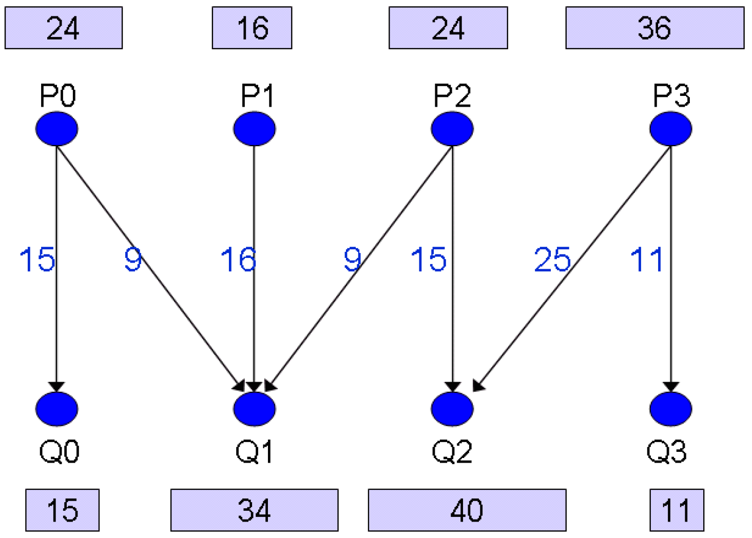
In a similar way, an irregular distribution GB (P, Q) is modeled by a weighted bipartite graph GGB(P, Q) = (S, T, E). For instance, in Figure 3, array elements A(1:100) are to be redistributed. Originally, array elements A(1:24), A(25:50), A(51:64), A(65:100) are mapped onto P0, P1, P2, and P3, respectively. After redistribution, a new distribution is formed, such as A(1:15), A(16:49), A(50:89), A(90:100) onto Q0, Q1, Q2, and Q3, respectively. Its distribution graph, GGB(4, 4), is presented in Figure 4. Note that one processor may need to send array elements to multiple consecutive processors in an irregular distribution. For example, P0 has 24 elements A(1:24) which A(1:15) are sent to Q0, and A(16:24) are sent to Q1. As a result, there is an edge with a weight 15 and another edge with a weight 9 in the distribution graph to indicate these two communications in Figure 4.
Most parallel computer programming languages supply run-time primitives or instructions to reallocate the array distribution of a program. Consequently, designing effective algorithms to do array redistribution is crucial for implementing distributed memory system software for these programming languages. In addition to array redistribution in parallel systems, in recent years, different data redistribution issues also received a lot of attention, including data redistribution in wireless sensor networks to minimize power consumption [5], data redistribution and retrieval in wireless sensor networks to preserve data [6], data redistribution in parallel join operations in distributed system [7], data distribution without breaking its semantics [8], data redistribution of data between processes [9], co-optimized application-level data movement and network-level data communications for distributed operators [10].
In this work, a bipartite graph is used to model data redistributions. Notice that a data redistribution is modeled by a bipartite graph G = (S, T, F), named a redistribution graph. In G, set S represents processor set containing a source to send data, and set T represents processor set containing a destination to receive the data, and each edge in F indicates the message. The interested data redistributions are modeled as the following graph problems in this work.
Definition 1.
For a bipartite graph G = (S, T, F) as an input, the maximum edge coloring problem (MECP) is to find a set of edge colorings (partitions) {F1, F2, F3, …, Fz} of F to minimize , where w(e) is the weight of edge e.
When a set of independent edges of the given graph G is used to represent a set of synchronized contention-free communications in MECP, the value max{w(e)|e∈Fi} indicates the longest time required to complete all communications allocated to ith step. Accordingly, the sum of max{w(e)|e∈Fi}(for 1 ≤ i ≤ z) is denoted as , which indicates the overall communication time for the data redistribution represented by G. In the next problem, we try to not only shorten the overall communication time but also the number of required communication steps. Additional variants of MECP use the minimum number of edge colorings, which are defined as follows.
Definition 2.
For a bipartite graph G = (S, T, F) as an input, the maximum degree edge coloring problem (MDECP) is to find out a set of edge colorings {F1, F2, F3, …, FΔ(G)} of G to minimize , where w(e) denotes the weight of e and Δ(G) denotes the maximum degree of G.
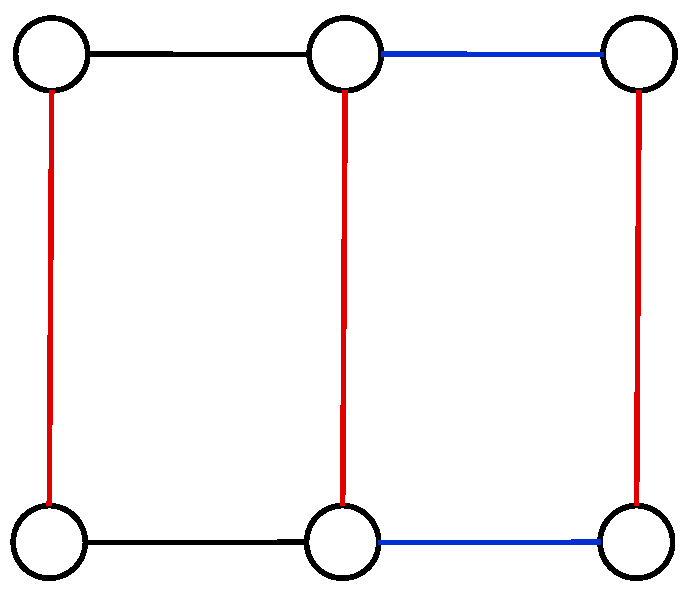
For example, when the input is the distribution graph G in Figure 4, a solution to the MECP is the edge partition {{Po, Q0}, {P1, Q1}, {P3, Q2}}, {{Po, Q1}, {P2, Q2}, {P3, Q3}}, and {{P1, Q1}} with the minimum value max{15, 16, 25} + max{9, 15, 11} + max{9} = 25 + 15 + 9 = 49, as shown in Figure 5. Since the number of colors used equals to the maximum degree of G, the edge partition is also a solution to the MDECP.
In previous research, the maximum coloring problem has been defined in [11,12]. The problem here is finding a proper coloring on the vertex set of input graphs such that the color classes (disjoint vertex sets) V1, V2, …, Vk minimize where w denotes the weight function and k denotes the number of colors used. However, the maximum coloring problem is an NP-hard problem even when its input is an interval graph [11]. Due to its intractability, a lot of papers aim to devise approximation algorithms for it on special graphs [11,12]. Obviously, the above problem is a kind of vertex coloring, which is totally different from the edge coloring problems defined in this work.
Note that some traditional open shop scheduling problems can be solved by using a bipartite-graph based approach [13]. A shop consists of many processors. Each of these processors performs a different task. In open shop no restrictions are placed on the order in which the tasks for any job are to be processed, which is different from the MECP and MDECP defined in this work. In [13], Gonzalez et al. showed that preemptive and non-preemptive optimal finish time schedules can be obtained in linear time when the number of processors is two. When the number of processors is larger than two, the optimal finish time schedule can still be obtained in polynomial time by applying maximal matching in bipartite graphs.
To the best knowledge of the authors, this is the first time anyone has set out to define MECP and MDECP by using bipartite graph terms and techniques. Though some sophisticated algorithms have been developed for MDECP [3,4,14], MECP and MDECP are open to scholars to devise a polynomial-time algorithm even when the input belongs to biplanar graphs. In this work, we present the first approximation algorithm for MECP with a ratio bound of two when the input graph is biplanar.
Moreover, a new graph problem called the cost-sharing maximum edge coloring problem (CSMECP) is defined in this work to further model how to partition communication messages in irregular redistribution scheduling. In our previous conference paper [15], we designed a heuristic algorithm to partition large data segments into multiple small data segments and to schedule them in different communication steps without using graph techniques. In this work, we formally reformulate the ideas by using a new graph decision problem, CSMECP. So far, it is an open question to know whether CSMECP is NP-complete or not. In this work, we also prove that the CSMECP is an NP-complete problem even when the input belongs to biplanar graphs.
In short, the contributions of this work are listed below.
- Define three new bipartite graph models including MECP, MDECP, and CSMECP.
- Design a first approximation algorithm with ratio bound of two for MECP when the input is a biplanar graph.
- Give a formal proof to show that the CSMECP is an NP-complete problem even when the input is a biplanar graph.
The remainder of our work is organized below. Section 2 introduces required graph definitions. Related research is briefly described and discussed in Section 3. We design and prove the correctness of an approximation algorithm for MECP in Section 4. Section 5 defines the CSMECP and shows that it is NP-complete. At last, Section 6 concludes this work and points out some future work.
2. Definitions and Notations
A tree is a connected acyclic graph. The components of a graph, G, are its maximal connected subgraphs. We use ω(G) to denote the number of components of G. Let N(v) denote the set of vertices adjacent to v. A multi-graph is a graph with two more edges with the same pair of ends. The degree dG(v) of a vertex v in a loopless graph G is the number of incident edges. The maximum degree of vertices of G is denoted by Δ(G).
A k-edge coloring of G = (V, E) is a labeling function f:E→S, where |S| = k. The labels are colors; the edges of one color form a color class. A k-edge-coloring is proper if incident edges have different labels. A graph is k-edge colorable if it has a proper k-edge-coloring. The edge chromatic number χ’(G) of a loopless graph G is the least k such that G is k-edge-colorable. For example, Figure 6 shows a graph that is 3-edge colorable; its edge chromatic number χ’(G) = 3.
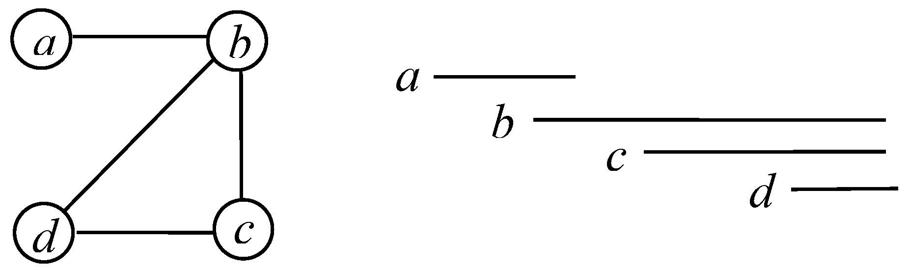
A matching in a graph G is a set of non-loop edges with no shared endpoints. A graph is bipartite if its vertex set is the union of two disjoint independent sets, called partite sets. A complete bipartite graph is a simple bipartite graph such that two vertices are adjacent if and only if they are in different partite sets; when the sets have sizes m and n, this complete bipartite graph is denoted by Km, n. The line graph of a graph G, written L(G), is the graph whose vertices are the edges of G, with (e, f) is in the edge set of L(G) when e = (u, v) and f = (v, w). In Figure 7, the right graph is the line graph L(G) of the left graph G.
G = (V, E) is an interval graph provided that one can assign to each vertex u an interval Iu such that Iu∩Iv is nonempty precisely when (u, v)∈E. For example, in Figure 8, the graph is an interval graph because there is a set of intervals representing vertex set.
A method for embedding a bipartite graph G = (X, Y, E) into two parallel lines is putting the vertices of X on the first line and the vertices of Y on the second line. For every edge (x, y) in G where x∈X and y∈Y, draw an interval from x to y. In the above embedding, if all edges do not cross, this bipartite graph is called biplanar [16]. A sequence of X(Y) owns the adjacency property if ∀ v in Y(X). A graph G = (X, Y, E) is called a doubly convex-bipartite graph when both sequences of X and Y have the adjacency property [17]. At last, most graph definitions used in the work can be found in [18].
For easy reference, all notations used in this work are listed in the Table 1.
3. Related Work
Regular data redistribution like the SCALAPACK library uses block-cyclic data distribution on a virtual grid of processors to achieve good load-balance on arrays and an equal memory usage between processors. Arrays are wrapped by blocks in all dimensions corresponding to the processor grid. Many algorithms and formulism for discussing regular array redistribution are classified into two types: (1) set identification; and (2) communication optimization. Ramaswamy et al. found a mathematical representation for redistribution, which belongs to the former [19]. Prylli et al. implemented their algorithm in the ScaLAPACK so as to go from a block cyclic distribution to another one [20]. Based on a generalized matrix formula, Park et al. devised an algorithm for array redistribution from cyclic(x) on source processors to cyclic(Kx) on destination processors [1]. Petitet et al. proposed various redistribution methods in BLOCK-CYCLIC fashion for a very special application which executed block-partitioned linear algebra algorithms on dense matrices [2]. Bandera et al. pointed out some characterizations of the sparse matrix redistribution and its related issues because of the use of compressed representations [21]. Hsu et al. proposed a new method to perform a BLOCK-CYCLIC array redistribution [22]. They also implemented the proposed method on an IBM SP2 parallel machine.
The second type concerns communication optimization techniques, including processor mapping techniques for reducing transmission overheads [23,24,25], a multistage approach for decreasing startup costs [26], scheduling algorithms for avoiding contention [14,27,28,29], and a strip-mining method for reducing communication and computational overheads [30].
On the other hand, with respect to irregular array redistribution, previous work has usually focused on indexing, message generation, or communication efficiency. Guo et al. first mentioned the problem of communication set generation for irregular applications [31]. They also devised optimization techniques for irregular array in nested loops. To decrease communication cost in GEN_BLOCK redistribution, Lee et al. [25] devised logical processor reordering methods on irregular array redistribution. In [3,4], Wang et al. designed a divide-and-conquer approach to execute irregular array redistribution. In [14], Yook et al. presented two-stage scheduling for relocation problems on a processor grid. Their proposed scheduling algorithm makes use of a spatial locality in message passing. Their algorithms have been implemented on CRAY T3E and IBM SP2.
In [15], Yu et al. presents an efficient algorithm to partition large messages into multiple small ones and schedules them by using the minimum number of steps without communication contention and, in doing so, reduces the overall redistribution time. When the number of processors or the maximum degree of the redistribution graph increases or the selected size of the messages is medium, the proposed algorithm can significantly reduce the overall redistribution time to 52%. In [15], Yu et al. failed to model their problem theoretically and did not discuss the intractability of the resolved problem. In this work, we formally reformulate the ideas by using a new graph decision problem. We also prove that the new graph problem is an NP-complete problem even when the input belongs to biplanar graphs.
4. Two-Approximation Algorithm for Irregular Data Redistribution Scheduling
In Theorem 1, we are going to formally prove that the corresponding graphs of GEN_BLOCK redistribution are biplanar graphs, which are a subclass of special bipartite graphs, called doubly convex-bipartite graphs [17].
Theorem 1.
The corresponding redistribution graph of GEN-BLOCK data redistribution is biplanar.
Proof.
Clearly the corresponding graph GGB(P, Q) = (S, T, E) is bipartite. The rest is to prove that it is planar. We can try to find out a biplanar embedding for GGB(P, Q) (see Figure 3 and Figure 4 for example) by placing all processors on two lines and numbering them from left to right (i.e., {P0, P1, …, P|P|−1} and {Q0, Q1, …, Q|Q|−1}). In the GEN-BLOCK format GB (P, Q), any set of consecutive array elements are originally allocated to consecutive source processors with respect to {P0, P1, …, P|P|−1}. Moreover, any set of consecutive array elements needs to be reallocated to consecutive destination processors with respect to {Qj, Qj+1, …, Qk}. As a result, when there is a message sent and reallocated from Pi to Qo(i), then for any j such that i ≤ j ≤ |P|−1 and any message sent from Pj to Qo(j), we have o(j) ≥ o(i). Suppose the corresponding redistribution graph is not biplanar, there is at least a pair of crossing edges such that (Pj, Qo(j)) and (Pj+Δ, Qo(j+Δ)) where Δ > 0 and o(j + Δ) < o(j). A contradiction occurs. Therefore, the corresponding redistribution bipartite graph is a biplanar graph. □
Theorem 2 presents extra properties of biplanar graphs, which will be used in this work.
Theorem 2.
- (1)
- A graph G is a biplanar graph.
- (2)
- After removing all leaves in G, the remainder is an acyclic graph and contains no vertices with a degree more than two.
- (3)
- A graph G contains a set of caterpillars which are disjoint graphs.
In Theorem 2, a caterpillar is a tree in which a single path (the spine) is incident to (or contains) every edge. When n denotes the number of vertices (i.e., |V|) in G, the edge set of a bipartite graph contains at most O(n2) edges. Yet, if the input is planar, the number of edges in G would be reduced to 3n − 6 [18]. Moreover, because biplanar graphs are essentially a subclass of planar graph, the number of edges in biplanar graphs is evidently less than 3n − 6. Additionally, by combining Theorem 1 with Theorem 2, we conclude that the graph generated from the GEN-BLOCK method is a forest in the following corollary. The next corollary further indicates that the number of edges in G is less than or equal to n − 1.
Corollary 1.
The graph G generated from GEN-BLOCK data redistribution is a forest.
Theorem 3.
For a redistribution graph G = (X, Y, E) of GEN-BLOCK data redistribution, we have that |E| = |X| + |Y| − ω(G), where ω(G) represents the number of components of G.
Proof.
Suppose that G consists of ω(G) trees T1, T2, …, Tω(G) (by Corollary 1). Since the size of edge set of a tree is one less than the size of its vertex set and G consists of ω(G) trees, we have |E| = |X| + |Y| − ω(G). □
Although we know that the redistribution graph constructed from GEN-BLOCK data redistribution is a biplanar graph by Theorem 1, so far there exists no polynomial time algorithm for MECP even when the input belongs to such graph. On the other hand, it becomes crucial to design an efficient approximation algorithm for MECP when the input is restricted to biplanar graphs. In order to devise such algorithm, we need to investigate the properties of the line graph L(G) of a biplanar graph G, because it is easy to see that the max-coloring problem on L(G) is equivalent to MECP on G. With the help of Theorem 2 and Corollary 1, we have found that G contains a set of caterpillars, which are useful to show that L(G) is an interval graph.
The next theorem becomes essential for us to design an approximation algorithm for the MECP latter.
Theorem 4.
The line graph of the communication graph of GEN-BLOCK data redistribution is an interval graph.
Proof.
When a connected communication graph G = (S, T, E) of GEN-BLOCK data redistribution is given as an input, we only need to find out an interval model of L(G). In view of the fact that G is biplanar (by Theorem 1), we can construct a biplanar embedding of G on two lines. Without changing the sequences of the biplanar embedding, we need to show that these sequences are able to be rescaled to satisfy the next four properties:
- Every vertex v in S∩T can be assigned and labeled with a distinct integer χ(v) from left to right where 1 ≤ χ(v) ≤ |S|+|T|. Moreover, the x-coordinate of vertex v on two horizontal lines is exactly χ(v).
- Vertex set S∩T can be grouped into two disjoint subsets: spine set B and leaf set L. Here B contains all vertices in the spine, and L contains the rest of vertices (that is, all vertices with degree one in G); that is, L contains all leaf nodes in G. Since every vertex v in L is a leaf, there is a unique edge (v, bk) connecting v to another vertex in B by Theorem 2.
- Suppose B={vb0, vb1, …, vb|B|−1} is sorted ascending by x-coordinate. Every vertex v in B is assigned with a unique integer χ(v) in interval [1, |S| + |T|]. Due to biplanar graph properties, the space between the two parallel lines is partitioned into |B| + 1 closure subspaces. Similarly, interval [1, |S| + |T|] can be partitioned into at most |B| + 1 subintervals [1, χ(vb0)], [χ(vb0), χ(vb1)], …, [χ(|B|−1), |S| + |T|] with respect to the x coordinates of vertices in B. Since G is a connected graph, there is an edge connecting every pair of neighboring vertices in spine set B.
- Due to the properties of bipartite planar graphs, L is able to be divided into R ≤ |B| disjoint leaf sets L1, L2, …, L|B| such that each vertex in the same leaf set is adjacent to the same vertex in B. We can rescale the biplanar drawing properly so that every vertex v in the same leaf set is allocated with a x-coordinate χ(v) contained in a same subintervals selected from [1, χ(vb0) − 1], [χ(vb0) + 1, χ(vb1) − 1], …, [χ(|B|−1) + 1, |S| + |T|]. Moreover, when two leaf nodes are in different leaf sets, their x-coordinates contained in different subintervals selected from [1, χ(vb0) − 1], [χ(vb0) + 1, χ(vb1) − 1], …, [χ(|B|−1) + 1, |S| + |T|] (e.g., blue dash rectangles in Figure 9). Also notice that for each edge (u, v) in this sequence, their corresponding x-coordinates χ(u) and χ(v) are located in the same subintervals selected from [1, χ(vb0)], [χ(vb0), χ(vb1)], …, [χ(|B|−1), |S| + |T|].
To show that L(G) is an interval graph, we need to find out its interval model. According to the above rescaled planar drawing, we first label each vertex of G with its x-coordinate, and then an interval [χ(v1) − 0.1, χ(v2) + 0.1] is constructed for every (v1, v2) in edge set (Figure 9). The rest shows that the intervals obtained represent L(G).
Assume there are two vertices adjacent in L(G) and its corresponding edges in G are e1 = (u, v1) and e2 = (u, v2). Without loss of generality, let χ(v1) < χ(v2). When χ(u) < χ(v1) < χ(v2), the interval [χ(u) − 0.1, χ(v1) + 0.1] (representing e1) intersects the interval [χ(u) − 0.1, χ(v2) + 0.1] (representing e2). On the other hand, When χ(v1) < χ(v2) < χ(u), the interval [χ(v1) − 0.1, χ(u) + 0.1] (representing e1) also intersects the interval [χ(v2) − 0.1, χ(u) + 0.1] (representing e2). When χ(v1) < χ(u) < χ(v2), the interval [χ(v1) − 0.1, χ(u) + 0.1] (representing e1) intersects the interval [χ(u) − 0.1, χ(v2) + 0.1] (representing e2).
Conversely, without loss of generality, when χ(u1) ≤ χ(u2) ≤ χ(v1) ≤ χ(v2) and {u1, u2}⊆S and {v1, v2}⊆T, we have a pair of overlapped intervals [χ(u1) − 0.1, χ(v1) + 0.1] and [χ(u2) − 0.1, χ(v2) + 0.1]. We claim that the corresponding two edges (u1, v1) and (u2, v2) are incident with a same vertex (either u1 = u2 or v1 = v2). Otherwise, we have u1 ≠ u2 and v1 ≠ v2 (similarly χ(u1) ≠ χ(u2) and χ(v1) ≠ χ(v2)), and the constructed intervals for the edges must be [χ(u1) − 0.1, χ(v1) + 0.1] and [χ(u2) − 0.1, χ(v2) + 0.1] where χ(u1) < χ(u2) < χ(v1) < χ(v2). Since χ(u1) and χ(v1) (similarly χ(u2) and χ(v2)) are in the same subintervals selected from [1, χ(vb0)], [χ(vb0), χ(vb1)], …, [χ(|B|−1), |S| + |T|]. That means χ(u1), χ(u2), χ(v1), χ(v2) are in the same subintervals selected from [1, χ(vb0)], [χ(vb0), χ(vb1)], …, [χ(v|B|−1), |S| + |T|]. As a result, at most one vertex of {u1, u2, v1, v2} is in B. Otherwise, if u1 and v2 are in B, then v1 and u2 should be adjacent to the same vertex. A contradiction occurs. Suppose only one vertex of {u1, u2, v1, v2} is in B, the remaining two leaf vertices should be adjacent to a same node in B. Another contradiction occurs. When χ(u2) < χ(u1) < χ(v1) < χ(v2), Without loss of generality, we have {u1, u2}⊆S and {v1, v2}⊆T. Then two edges (u1, v1) and (u2, v2) are crossing in the biplanar graph drawing. A contradiction occurs.
At last, the constructed interval model represents L(G), and finally we prove that the line graph of a communication graph of GEN-BLOCK data redistribution is an interval graph. □
We devise an approximation algorithm for maximum edge coloring problem (called AMECP) listed below.
| Algorithm AMECP: |
| Input: G =(X, Y, E) of GEN-BLOCK. |
| Output: an edge coloring {F1, F2, F3, …, Fz} of G and . |
| 1: Construct L(G) from G. |
| 2: Find out an interval representation for L(G) by executing the recognition algorithm of interval graphs based on Theorem 4. |
| 3: Construct a vertex coloring {V1, V2, V3, …, Vz} of L(G) by executing an algorithm to solve the maximum coloring problem for interval graphs. |
| 4: Construct an edge coloring {F1, F2, F3, …, Fz} of G from vertex coloring {V1, V2, V3, …, Vz}, and calculate . |
The correctness and time complexity of AMECP are discussed and provided in Theorems 5 and 6.
Theorem 5.
AMECP is an approximation algorithm with a ratio bound of two for MECP when the input is a biplanar graph.
Proof.
Because an edge coloring of G is always mapped to a vertex coloring of L(G), the MECP of G is converted to the maximum coloring problem of L(G) according to the mapping. Due to the fact that L(G) is an interval graph (proved in Theorem 4), an approximation algorithm with a ratio bound of two for MECP of G can be devised by executing Pemmaraju et al.’s algorithm [11], which found a relation between maximum coloring and on-line graph coloring and exploited this observation to design an approximation algorithm for max vertex coloring on interval graphs. At last, we show AMECP is an approximation algorithm with a ratio bound of two for MECP. □
Theorem 6.
AMECP takes O(n2) time, where n = |X| + |Y|.
Proof.
Algorithm AMECP is analyzed here step by step. The first step takes O(n2) time because to implement it we need to compare every pair of edges in E of G to create the edge set of L(G). By Theorem 3, |E| = |X| + |Y| − ω(G). That means |E| < n, because ω(G) ≥ 1. As a result, this step takes at most (n − 1) × (n − 2)/2 = O(n2) computation time. The second step can be implemented in an efficient way (O(n2) time) if we apply Booth and Lueker’s interval graph recognition algorithm, which adopted well-known PQ trees to test the consecutive ones property [34]. The third step needs O(nlog n) time if applying Pemmaraju et al.’s two-approximation algorithm [11]. At last, the last step can be implemented in linear time trivially. Finally, AMECP takes O(n2) time totally. □
5. New Graph Model for Applying Partitioning Message Techniques
In order to solve the CSMECP efficiently, we try to shorten the total communication time but do not increase the required total steps simultaneously. In [15], Yu et al. have designed a heuristic algorithm for the CSMECP. Unlike existing conventional approaches, the intuitive idea behind our previous work [15] is partitioning larger data into multiple small data units, and our algorithm reschedules these added small data units properly in different existing steps. So far, it is an open question to know whether CSMECP is NP-hard or not. In this section, we give a proof for CSMECP.
When G is bipartite, χ′(G) = Δ(G) is a well-known graph property [18]. In terms of graphs, this equation indicates the number of minimum colors is equal to the maximum degree of the inputted bipartite graph. In terms of communication, this equation indicates that the minimum number of communication steps for this distribution (discussed in this work) equals the maximum degree Δ(G) of the corresponding distribution graph G. Specifically, to avoid increasing the total communication steps, we should partition larger data into small data units as many as possible and scatter them into different steps if Δ(G) = Δ(G’) here G’ represents the new distribution graph after these partitions. How to scatter these new add-in small data elements into different steps is another key issue for CSMECP. When a new data communication is added in a pre-schedule for an arbitrary step, if the size of the new data unit is larger than that of every data units in the pre-schedule, the time for this step becomes longer. Note that CSMECP is designed to avoid this case.
In CSMECP, to model how to partition larger data into small data units, we add duplicate edges for each of these edges with larger weights to the redistribution graph. For such edge e with larger weight, these corresponding new-adding edges share weights with e. The above techniques are used to present the properties of CSMECP as follows.
Property 1.
When a weighted biplanar graph G = (S, T, E) is taken as an input, the CSMECP is a kind of decision problem, which adds additional edges E′ so that the new graph G′ = (S, T, E∪E′) satisfies the subsequent constraints:
- 1.
- Additional edge (s, t) is allowed to be added in edge set E′ only if these two end points, s and t, are originally adjacent by an edge (s, t) in E.
- 2.
- Δ(G′) = Δ(G). That means after adding some multiple edges, the maximum degree of the new graph G′ remains unchanged when compared to that of the original one G.
- 3.
- In G′ = (S, T, E∪E′), = in G = (S, T, E), where w(e) is the weight of e.
When a weighted bipartite graph G = (S, T, E) with a value K are given as inputs, the cost-sharing maximum edge coloring problem (CSMECP) is to answer whether there is a proper edge coloring {F1, F2, F3, …, FΔ} of G′ = (V, E∪E′) such that ≤ K.
In the rest of this section, we show that CSMECP is NP-complete even when G is biplanar by transforming the partition problem to CSMECP.
Property 2.
When a set A with a function s(k)∈Z+ for each k∈A are given as inputs, the partition problem is to answer whether there exists a subset A* in A such that .
Theorem 7.
CSMECP is NP-complete even when the input is a biplanar graph.
Proof.
First, to prove that CSMECP∈NP is obvious, because a nondeterministic procedure is easily devised to guess the added edges E′ and their shared weights, and then the algorithm checks whether the above three conditions in Property 1 are satisfied.
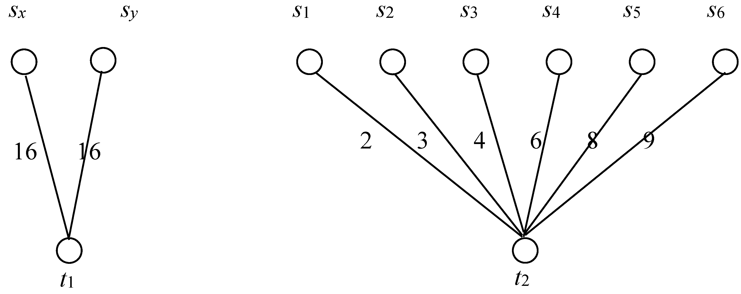
Next, we reduce the partition problem, which has been found to be NP-complete in [35], to CSMECP. When an instance of the partition problem A = {α1, α2, …, αn} with a weight function s(α) for each αi∈A are given as inputs, we generate a graph G=(S, T, E) so that
- vertex set S = {sx, sy, s1, s2, …, sn} and T = {t1, t2},
- edge set E = {(sx, t1), (sy, t1), (s1, t2), (s2, t2), …, (sn, t2)}, and
- the weights of (sx, t1) and (sy, t1) are /2, and the weight of (si, t2) is s(αi) for all αi in A.
Figure 10 depicts the constructed bipartite graph from an instance of the partition problem A = {2, 3, 4, 6, 8, 9} with n = 6. The graph G=(S, T, E) can be obtained by the above construction, where S={sx, sy, s1, s2, …, s6}, T = {t1, t2}, and E = {(sx, t1), (sy, t1), (s1, t2), (s2, t2), …, (s6, t2)}. The associated weights of (sx, t1) and (sy, t1) are 16 = (2+3+4+6+8+9)/2, and each of the remaining edges is assigned with a distinct element (value) in A.
It is also obvious to demonstrate that the above reduction is able to be executed in O(nk) time where k is a constant. The rest is to find out that there is a subset A* in A so that if there is an edge coloring {E1, E2, E3, …, EΔ(G′)} of G′ = (S, T, E∪E′) and ≤ K = .
Assume that there is a subset A* = {αr(1), αr(2), …, αr(k)}⊆A = {αr(1), αr(2), …, αr(n)} such that , obviously = ()/2 = K/2. We can then construct a weighted biplanar graph G = (S, T, E) accordingly. Assume that the extra added edges E′ consist of k − 1 copies of (sx, t1) and n – k − 1 copies of (sy, t1). As a result, Δ(G′) and Δ(G) all equal n. Because = ()/2 = K/2 and , we distribute {s(αr(1)), s(αr(2)), …, s(αr(k))} to k copies of (sx, t1) and {s(αr(k+1)), s(αr(k+2)), …, s(αr(n))} to n − k copies of (sy, t1). There exists a coloring for edges {E1, E2, E3, …, En} of G′ = (S, T, E∪E′) where Ei = {(sx, t1), (sr(i), t2)} for 1 ≤ i ≤ k and Ei = {(sy, t1), (sr(j), t2)} for k + 1 ≤ j ≤ n. Evidently, = = K.
Figure 11 shows an edge coloring of G′ which is generated according to G. Since A* = {2, 6, 8}⊆A = {2, 3, 4, 6, 8, 9} such that 2 + 6 + 8 = 3 + 4 + 9 = 16. We distribute {2, 6, 8} to three copies of (sx, t1) and {3, 4, 9} to three copies of (sy, t1).
On the other hand, assume that there exists an edge coloring {E1, E2, E3, …, EΔ(G′)} of G′ so that ≤K = . According to the previous construction of G, the weights of (sx, t1) and (sy, t1) equal /2. Let A*⊆A contains the corresponding elements of the edges, which are adjacent to t2 and scheduled with the copies of (sx, t1). Similarly, A-A* contains the corresponding elements of the edges, which are adjacent to t2 and scheduled with the copies of (sy, t1). We claim that = K/2. Otherwise, for any edge coloring, we always have either > K/2 or > K/2. Without a loss of generality, assume that > K/2 and the cost to schedule A* is greater than K/2. On the other hand, the cost to schedule A-A* is not less than K/2 because the cost distributed to the copies of (sy, t1) is K/2. As a result, > K. A contradiction occurs. □
6. Conclusion and Future Work
We have defined MECP, MDECP, and CSMECP graph models in this work. In addition, the intractability of CSMECP has been formally proved, and we also devised a two-approximation algorithm for MECP when the input is a biplanar graph. Note that, by applying bipartite graph techniques, an efficient heuristic algorithm including three steps to decrease the total redistribution time has been devised in our previous work [15]. Moreover, in [15], extensive simulation results are presented for the proposed heuristic algorithm for CSMECP. In future, how to estimate the reduction ratio precisely and formally is a big challenge to us. The bipartite graph techniques devised and defined in the work including MECP, MDECP, and CSMECP are expected to be applied to other practical problems in different distributed systems and networks.
Author Contributions
Conceptualization, C.W.Y. and Q.L.; methodology, C.W.Y.; software, Q.L.; validation, C.W.Y. and Q.L.; formal analysis, C.W.Y.; investigation, Q.L.; resources, Q.L.; writing—original draft preparation, C.W.Y.; writing—review and editing, Q.L.; visualization, Q.L.; supervision, C.W.Y.; project administration, Q.L.; funding acquisition, Q.L.
Funding
Q.L. was partially founded by Research Project of Zhejiang Province (Grant No. Y201636885).
Conflicts of Interest
The authors declare no conflict of interest.
References
- Park, N.; Prasanna, V.K.; Raghavendra, C.S. Efficient Algorithms for Block-Cyclic Data Redistribution Between Processor Sets. IEEE Trans. Parallel Distrib. Syst. 1999, 10, 1217–1240. [Google Scholar] [CrossRef]
- Petitet, A.P.; Dongarra, J.J. Algorithmic Redistribution Methods for Block-Cyclic Decompositions. IEEE Trans. PDS 1999, 10, 1201–1216. [Google Scholar] [CrossRef]
- Wang, H.; Guo, M.; Wei, D. Divide-and-conquer Algorithm for Irregular Redistributions in Parallelizing Compilers. J. Supercomput. 2004, 29, 157–170. [Google Scholar] [CrossRef]
- Wang, H.; Guo, M.; Chen, W. An Efficient Algorithm for Irregular Redistribution in Parallelizing Compilers. In Lecture Notes in Computer Science, Proceedings of 2003 International Symposium on Parallel and Distributed Processing with Applications, Aizu-Wakamatsu, Japan, 2–4 July, 2003; Springer: Berlin/Heidelberg, Germany, 2003; Volume 2745, pp. 76–87. [Google Scholar]
- Tang, B.; Jaggi, N.; Wu, H.; Kurkal, R. Energy-efficient data redistribution in sensor network. In Proceedings of the 7th IEEE International Conference on Mobile Ad-hoc and Sensor Systems, San Francisco, CA, USA, 8–12 November 2010; pp. 352–361. [Google Scholar]
- Yi, Q.; Wang, J.; Liu, C. Energy-efficient data storage solutions under sink failures. In Proceedings of the 10th International Conference on Communications and Networking in China, Shanghai, China, 15–17 August 2015; pp. 349–354. [Google Scholar]
- Cheng, L.; Li, T. Efficient data redistribution to speed up big data analytics in large systems. In Proceedings of the 2016 IEEE 23rd International Conference on High Performance Computing, Hyderabad, India, 19–22 December 2016; pp. 91–100. [Google Scholar]
- Dreher, M.; Peterka, T. Bredala: Semantic data redistribution for in situ applications. In Proceedings of the 2016 IEEE International Conference on Cluster Computing, Taipei, Taiwan, 12–16 September 2016; pp. 279–288. [Google Scholar]
- Marrinan, T.; Insley, J.A.; Rizzi, S.; Tessier, F.; Papka, M.E. Automated dynamic data redistribution. In Proceedings of the 2017 IEEE International Parallel and Distributed Processing Symposium Workshops, Lake Buena Vista, FL, USA, 29 May–2 June 2017; pp. 1208–1214. [Google Scholar]
- Cheng, L.; Wang, Y.; Pei, Y.; Epema, D. A Coflow-Based Co-Optimization Framework for High-Performance Data Analytics. In Proceedings of the 2017 46th International Conference on Parallel Processing (ICPP), Bristol, UK, 14–17 August 2017; pp. 392–401. [Google Scholar]
- Pemmaraju, S.V.; Raman, R.; Varadarajan, K.R. Buffer minimization using max-coloring. In Proceedings of the Fifteenth Annual ACM-SIAM Symposium on Discrete Algorithms, Philadelphia, PA, USA, 11–14 January 2004; pp. 562–571. [Google Scholar]
- Pemmaraju, S.V.; Raman, R. Approximation algorithms for the max-coloring problem. In Lecture Notes in Computer Science, Proceedings of the International Colloquium on Automata, Languages, and Programming, Lisbon, Portugal, 11–15 July 2005; Springer: Berlin/Heidelberg Germany, 2015; Volume 3580, pp. 1064–1075. [Google Scholar]
- Gonzales, T.; Sahni, S. Open shop scheduling to minimize finish time. J. ACM 1976, 23, 665–679. [Google Scholar] [CrossRef]
- Yook, H.G.; Park, M.-S. Scheduling GEN_BLOCK Array Redistribution. J. Supercomput. 2002, 2, 251–267. [Google Scholar] [CrossRef]
- Yu, C.W.; Hsu, C.-H.; Yu, K.-M.; Lian, C.K.; Chen, C.-I. Irregular Redistribution Scheduling by partitioning Messages. In Lecture Notes in Computer Science, Proceedings of the 10th Asia-Pacific Computer Systems Architecture Conference, Singapore, 24–26 October 2005; Springer: Berlin/Heidelberg, Germany, 2005; Volume 3740, pp. 295–309. [Google Scholar]
- Yu, C.W. On the complexity of the maximum biplanar subgraph problem. Inf. Sci. 2000, 129, 239–250. [Google Scholar] [CrossRef]
- Yu, C.W.; Chen, G.H. Efficient parallel algorithms for doubly convex-bipartite graphs. Theor. Computer Sci. 1995, 147, 249–265. [Google Scholar] [CrossRef] [Green Version]
- Bondy, J.A.; Murty, U.S.R. Graph Theory with Applications; Macmillan: London, UK, 1976. [Google Scholar]
- Ramaswamy, S.; Simons, B.; Banerjee, P. Optimization for Efficient Data redistribution on Distributed Memory Multicomputers. J. Parallel Distrib. Comput. 1996, 38, 217–228. [Google Scholar] [CrossRef]
- Prylli, L.; Touranchean, B. Fast runtime block cyclic data redistribution on multiprocessors. J. Parallel Distrib. Comput. 1997, 45, 63–72. [Google Scholar] [CrossRef]
- Bandera, G.; Zapata, E.L. Sparse Matrix Block-Cyclic Redistribution. In Proceedings of the Proceedings 13th International Parallel Processing Symposium and 10th Symposium on Parallel and Distributed Processing, San Juan, PR, USA, 12–16 April 1999. [Google Scholar]
- Hsu, C.-H.; Bai, S.-W.; Chung, Y.-C.; Yang, C.-S. A Generalized Basic-Cycle Calculation Method for Efficient Array Redistribution. IEEE Trans. Parallel Distrib. Syst. 2000, 11, 1201–1216. [Google Scholar]
- Hsu, C.-H.; Yang, D.-L.; Chung, Y.-C.; Dow, C.-R. A Generalized Processor Mapping Technique for Array Redistribution. IEEE Trans. Parallel Distrib. Syst. 2001, 12, 743–757. [Google Scholar]
- Kalns, E.T.; Ni, L.M. Processor Mapping Technique Toward Efficient Data Redistribution. IEEE Trans. Parallel Distrib. Syst. 1995, 6, 1234–1247. [Google Scholar] [CrossRef]
- Lee, S.; Yook, H.; Koo, M.; Park, M. Processor reordering algorithms toward efficient GEN_BLOCK redistribution. In Proceedings of the ACM Symposium on Applied Computing, Las Vegas, NV, USA, March 2001; pp. 539–543. [Google Scholar]
- Kaushik, S.D.; Huang, C.H.; Ramanujam, J.; Sadayappan, P. Multiphase data redistribution: Modeling and evaluation. In Proceedings of the 9th International Parallel Processing Symposium, Santa Barbara, CA, USA, 25–28 April 1995; pp. 441–445. [Google Scholar]
- Desprez, F.; Dongarra, J.; Petitet, A. Scheduling Block-Cyclic Data redistribution. IEEE Trans. Parallel Distrib. Syst. 1998, 9, 192–205. [Google Scholar] [CrossRef]
- Guo, M.; Nakata, I.; Yamashita, Y. Contention-Free Communication Scheduling for Array Redistribution. Parallel Comput. 2000, 26, 1325–1343. [Google Scholar] [CrossRef]
- Lim, Y.W.; Bhat, P.B.; Prasanna, V.K. Efficient Algorithms for Block-Cyclic Redistribution of Arrays. Algorithmica 1999, 24, 298–330. [Google Scholar] [CrossRef]
- Wakatani, A.; Wolfe, M. Optimization of Data redistribution for Distributed Memory Multicomputers. short communication. Parallel Comput. 1995, 21, 1485–1490. [Google Scholar] [CrossRef]
- Guo, M.; Pan, Y.; Liu, Z. Symbolic Communication Set Generation for Irregular Parallel Applications. J. Supercomput. 2003, 25, 199–214. [Google Scholar] [CrossRef]
- Eades, P.; McKay, B.D.; Wormald, N.C. On an edge crossing problem. Available online: http://users.cecs.anu.edu.au/~bdm/papers/EdgeCrossing.pdf (accessed on 15 May 2019).
- Tomii, N.; Kambayashi, Y.; Shuzo, Y. On planarization algorithms of 2-level graphs. Tech. Group. Elect. Comp. IECEJ 1977, 38, 1–12. [Google Scholar]
- Booth, K.S.; Lueker, G.S. Testing for the consecutive ones property, interval graphs, and graph planarity using PQ-tree algorithms. J. Comput. Syst. Sci. 1976, 13, 335–379. [Google Scholar] [CrossRef] [Green Version]
- Garey, M.R.; Johnson, D.S. Computers and Intractability: A guide to the Theory of NP-completeness; Freeman: San Francisco, CA, USA, 1978. [Google Scholar]
Figure 1.
An example for BC(1, 4, 4).

Figure 2.
GBC(1, 4, 4) is K4, 4.

Figure 3.
An example for GB(4, 4).


Figure 5.
A solution to the maximum edge coloring problem (MECP) (and maximum degree edge coloring problem (MDECP)) when the input is the distribution graph in Figure 4.
Figure 5.
A solution to the maximum edge coloring problem (MECP) (and maximum degree edge coloring problem (MDECP)) when the input is the distribution graph in Figure 4.

Figure 6.
A graph G is 3-edge colorable.

Figure 7.
A graph G (left) with its line graph L(G) (right).

Figure 8.
An interval graph.

Figure 9.
A redistribution graph G with the intervals of L(G).

Figure 10.
An example of cost-sharing maximum edge coloring problem (CSMECP) constructed from an instance of the partition problem A = {2, 3, 4, 6, 8, 9} with n = 6.
Figure 10.
An example of cost-sharing maximum edge coloring problem (CSMECP) constructed from an instance of the partition problem A = {2, 3, 4, 6, 8, 9} with n = 6.

Figure 11.
An edge coloring of G’ generated from G.


Table 1.
Notations used in this work.
| Notations | Descriptions |
|---|---|
| n | the number of vertices in the input graph G |
| dG(v) | the number of incident edges to vertex v in a graph G |
| L(G) | the line graph of G |
| N(v) | the set of vertices adjacent to vertex v |
| w(e) | the weight of edge e |
| Δ(G) | the maximum degree of vertices of G |
| ω(G) | the number of components of G |
| χ’(G) | the edge chromatic number of G |
| z | the number of used colors |
| GBC(α,β, P, Q) | the distribution graph of BLOCK-SYCLIC array redistribution using Block-Cyclic(α) to Block-Cyclic(β) (from P processors to Q processors) |
| GGB(P, Q) | the distribution graph of GEN_BLOCK redistribution from P processors to Q processors |
© 2019 by the authors. Licensee MDPI, Basel, Switzerland. This article is an open access article distributed under the terms and conditions of the Creative Commons Attribution (CC BY) license (http://creativecommons.org/licenses/by/4.0/).
Share and Cite
MDPI and ACS Style
Li, Q.; Yu, C.W. New Bipartite Graph Techniques for Irregular Data Redistribution Scheduling. Algorithms 2019, 12, 142. https://doi.org/10.3390/a12070142
AMA Style
Li Q, Yu CW. New Bipartite Graph Techniques for Irregular Data Redistribution Scheduling. Algorithms. 2019; 12(7):142. https://doi.org/10.3390/a12070142
Chicago/Turabian StyleLi, Qinghai, and Chang Wu Yu. 2019. "New Bipartite Graph Techniques for Irregular Data Redistribution Scheduling" Algorithms 12, no. 7: 142. https://doi.org/10.3390/a12070142
Note that from the first issue of 2016, this journal uses article numbers instead of page numbers. See further details here.