Pruning Optimization over Threshold-Based Historical Continuous Query

Abstract

With the increase in mobile location service applications, spatiotemporal queries over the trajectory data of moving objects have become a research hotspot, and continuous query is one of the key types of various spatiotemporal queries. In this paper, we study the sub-domain of the continuous query of moving objects, namely the pruning optimization over historical continuous query based on threshold. Firstly, for the problem that the processing cost of the Mindist-based pruning strategy is too large, a pruning strategy based on extended Minimum Bounding Rectangle overlap is proposed to optimize the processing overhead. Secondly, a best-first traversal algorithm based on E3DR-tree is proposed to ensure that an accurate pruning candidate set can be obtained with accessing as few index nodes as possible. Finally, experiments on real data sets prove that our method significantly outperforms other similar methods.

1. Introduction

With the rapid development of mobile networks and positioning technologies, the trajectory data of mobile objects can be more conveniently obtained. For example, the Automatic Identification System is used to report the real-time location information of ships, and the mobile social applications are used to share the real-time location, etc. The trajectory data of mobile objects contains a large amount of information that can be analyzed and mined. By managing the trajectory data of mobile objects through mobile object database [1], a large number of applications based on location services can be promoted, such as geographic information systems, navigation systems, path planning systems, etc. Therefore, the performance of a mobile object database will determine the service capabilities that the location-based applications can provide.

In the past ten years, the research on mobile object database has achieved a lot of results, covering all aspects of data storage, management, query, and mining. Mobile object query is one of the key technologies of a mobile object database. In different scenarios, various types of query operations are needed to provide service support. Research on how to provide high-performance queries is the key to improving the service capability of a mobile object database. Therefore, it is important to implement a query operation that can accurately return the results in a short time. With the gradual deepening of research, people not only consider the spatial information of the moving object when querying, but also temporal information will be taken into account. At this stage, the query operations for the moving object include spatiotemporal range query, trajectory similarity query, neighbor query, threshold-based query [2], etc. We consider the following query requests for the historical trajectory data:

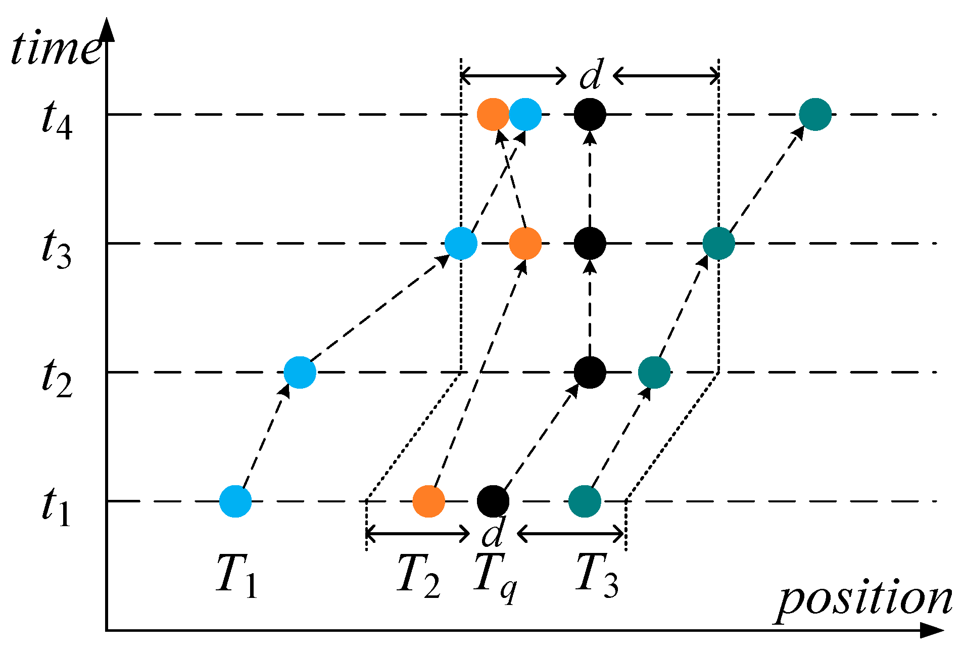
• Find which ships were within one nautical mile from the berth O₁ at any time instance of the time period from 10:00 on 11 November 2015 to 10:00 on 12 November 2015.
• Find which ships were within one nautical mile from the ship O₂ at any time instance of the time period from 8:00 on 12 November 2015 to 8:00 on 13 November 2015.

The above two queries require the query results at any time instance of the query time period, wherein the query request (1) takes a static object as the reference, and the query request (2) takes a moving object as the reference, both of which can be characterized as continuous queries [3]. However, there is a certain difference between these continuous queries and the traditional continuous ones. The traditional continuous query submits the query request to the database at once and remains active, and the query results are periodically returned until the predetermined query lifetime ends. While the query requests (1) and (2) demand the database to return all query results at once. It can be seen that these continuous queries face a greater data processing scale challenge than the traditional ones. In addition, we can see from the query conditions that the above query requests are constrained by the spatial distance threshold, so we call them threshold-based historical continuous queries (THC queries).

Figure 1 displays an example of THC query, where T_q is the historical trajectory of the query moving object O_q, and T₁, T₂, and T₃ are the historical trajectories of the moving objects O₁, O_2, and O₃, respectively, and the query time interval is (t₁, t₄), the distance threshold is d. As time goes by, the position of the moving object will change continuously. Hence, the query time interval can be subdivided into a plurality of smaller time segments, and the query results in each time segment are not the same. As Figure 1 shows, the results are O₂ and O₃ at the time interval (t₁, t₃), O₁, O₂ and O₃ at time instance t₃, O_1, and O₂ at the time interval (t₃, t₄).

THC queries can be processed by the classic “pruning-refinement” method [4]. In the pruning step, a certain pruning strategy is used to roughly check whether the trajectory data in the moving object database satisfies the constraint condition, and the trajectory data that does not match the condition is eliminated, and finally, a candidate set of trajectory data is obtained. The entire pruning process is usually performed by traversing a spatiotemporal index. In the refinement step, the candidate set is further filtered by the distance calculation, and the results that finally satisfy the query condition are returned to the user.

In the above process, the pruning step has a decisive influence on the overall query performance. This is because, first, the time overhead of pruning is an important part of the overall query time. If the pruning strategy can be optimized, and the processing time can be reduced, the overall query performance will undoubtedly be improved effectively. Second, the candidate set of pruning directly affects the performance of refinement. The closer the candidate trajectory data generated by pruning is to the final result, the less the number of trajectory distance calculations required in the refinement step, and the I/O times and the calculation time required for the query can be reduced effectively. In view of this, in order to achieve efficient query performance, we optimized the pruning step of THC queries. First, the pruning strategy based on extended Minimum Bounding Rectangle (MBR) overlap is proposed to reduce the processing overhead of a single pruning check. Secondly, we designed an extended 3DR-tree [5] structure called E3DR-tree to the index query object, and based on this, we implemented a best-first traversal algorithm, so that an accurate pruning candidate set was obtained with accessing as few nodes as possible in the traversal of the indexes.

Our main contributions can be summarized as follows:

• We propose a pruning strategy based on extended MBR overlap to optimize the single pruning check, thereby effectively reducing the processing time.
• We introduce a best-first traversal algorithm based on E3DR tree, to obtain a precise pruning candidate set for refinement processing under the premise of effectively controlling the number of accessed nodes when traversing the indexes.
• We evaluate our method with the dataset of ship trajectory, the experimental results verify the efficiency.

Section 2 introduces the related work. The background is introduced in Section 3. The method of pruning optimization is described in Section 4. Section 5 provides an experimental study of our method. Finally, we give a brief conclusion in Section 6.

2. Related Work

At present, there are many studies on historical continuous query, in addition to threshold-based historical continuous query, it also includes k nearest neighbor historical continuous query.

Frentzos et al. [6] introduced a depth-first traversal algorithm to support k nearest neighbor history continuous query and proposes a new line-to-rectangular Mindist (minimum distance) calculation method [7] to improve pruning efficiency. Moreover, they apply the above method in the two index structures of TB-tree [8] and 3DR-tree and verify the feasibility on the real and synthetic data sets.

Güting et al. [9] researched pruning optimization of k nearest neighbor historical continuous query. They propose an extended 3DR-tree structure to quickly determine the number of candidate trajectories, design a time-based index named BB-tree to achieve high-precision pruning, and based on this, implement a breadth-first large-scale node traversal algorithm to efficiently obtain candidate trajectory data.

Gowanlock et al. [10] conducted a study on threshold-based historical continuous query. In order to reduce the I/O overhead for query processing, they propose a memory-based R-tree structure to index the trajectory data and use a query algorithm based on MBR overlap to process the pruning and refinement. Compared to the first two studies, this study does not focus on the improvement of the algorithm but does a lot of experiments on real datasets to determine the appropriate parameters for the construction of memory-based R-tree. In addition, they also explore the parallelization of query based on OpenMP [11].

Huang et al. [12] propose a new threshold-based historical continuous query operation. For this query operation, a pruning method based on Mindist-Maxdist (minimum distance-maximum distance) and a refinement method based on dynamic time warping are introduced. In addition, this study also discusses the impact of trajectory segmentation on query and evaluates the performance of the query algorithm on the indexes of 3DR-tree, TB-tree and SETI [13], respectively.

With the rapid development of GPU technology, a series of methods [14,15,16] which use GPU to process the threshold-based historical continuous queries in parallel are proposed. On the one hand, considering that the GPU does not have branch prediction capabilities, these methods avoid using the tree-like structure to index the trajectory data, using the grid structure instead. On the other hand, considering that the GPU memory is limited, different from the snapshot queries taken by the above four methods, these methods divide the trajectory data contained in the mobile object database into multiple batches and iteratively process them.

Aside from the GPU-based methods, the above methods have more or less the following shortcomings: (1) Calculating the values of Mindist or Maxdist requires high computational costs [6,9,12]. (2) During the pruning step, the pruning candidate set generated by taking the whole query trajectory as a whole is not accurate enough [6,12]. Conversely, the pruning method that takes each segment of the query trajectory as a basic unit can obtain a more accurate candidate set, but the number of the accessed nodes is greatly increased [9,10]. In response to these two shortcomings, we will discuss the solutions in detail later.

3. Background

The real trajectory of the moving object is a continuous curve in space and time, but the sampling and storage of the trajectory data are carried out in discrete form, this is because the sensor device can only collect and send discrete samples. For example, a taxi equipped with a GPS device reports its position information every 10 s. The discrete position samples of a moving object constitute an ordered sequence of segments. When the sampling frequency is high enough, this sequence of segments can be relatively accurately approximated to the real trajectory of the moving object. Therefore, we used a segment-based data model to represent the trajectory of a moving object, defined as follows:

Definition 1.

The trajectory T of a moving object contains a sequence of trajectory segments (l₁, l₂, …, l_M) arranged chronologically. Each trajectory segment l records the linear motion of a moving object in a time interval, which can be expressed as $l=\{oid,p_s,p_e,t_s,t_e\},(t_s\le t_e)$, where oid is the identifier of the moving object and it can represent the moving object, p_s and p_e respectively represent the spatial position of the moving object at time instance t_s and t_e.

According to the data model of trajectory described in Definition 1, the spatial position of the moving object at a certain historical time instance can be obtained by linear interpolation. In the two-dimensional Euclidean space, given a trajectory segment $l=\{oid,p_s,p_e,t_s,t_e\}$, the spatial coordinates of p_s and p_e are expressed as $p_s=(q_{s1},q_{s2})$ and $p_e=(q_{e1},q_{e2})$, let $loc(t,oid)$ represent the spatial position of oid at the time instance t, and $lo{c}_k(t,oid)$ denote the k-th dimension coordinate of $loc(t,oid)$. For any time instance t in the time interval $[t_s,t_e]$, We compute the value of $lo{c}_k(t,oid)$ as

$$lo{c}_k(t,oid)=\{\begin{array}{ll}\frac{q_{ek}-q_{sk}}{t_e-t_s}(t-t_s)+q_{sk}& t_s<t_e\\ q_{sk}& t_s=t_e\end{array}.$$

(1)

Using Formula (1), we can calculate the spatial positions of two moving objects at a timestamp, and then obtain the distance between them. In this paper, we used Euclidean distance as the distance metric, let $d(loc(t,oi{d}_1),loc(t,oi{d}_2))$ denote the distance between oid₁ and oid₂ in the time instance t, according to the Euclidean distance formula

$$d(loc(t,oi{d}_1),loc(t,oi{d}_2))=\sqrt{{\displaystyle \sum _{k=1}^2{(lo{c}_k(t,oi{d}_1)-lo{c}_k(t,oi{d}_2))}^2}}.$$

(2)

In the two query requests listed in Section 1, the stationary object can be taken as a moving object that stays in a spatial position, so a uniform query definition can be given.

Definition 2.

Given a moving object oid_q, a moving object database D, a time interval [t_sq,t_eq], a distance threshold d, the historical trajectory T_q of oid_q in [t_sq,t_eq], the threshold-based historical continuous query return a collection of query results Rs, the element re of Rs is expressed as a tuple (ti, oids), where ti is a time interval, and oids is a set of moving objects. Rs satisfies the following two conditions:

(1) Given two elements$r{e}_1,r{e}_2\in Rs$, such that$r{e}_1.ti\cap r{e}_2.ti=\varnothing$and$r{e}_1.ti,r{e}_2.ti\subseteq [t_{sq},t_{eq}]$.

(2) Given an element$r{e}_1\in Rs$, a time instance$t_1\in r{e}_1.ti$, a moving object$oi{d}_1\in r{e}_1.oids$, such that$d(loc(t_1,oi{d}_1),loc(t_1,oi{d}_q))\le d$.

With other words, the time intervals of different Rs elements do not overlap, and the time interval of any Rs element must be within the query time interval. Moreover, the distance between each oid in Rs.oids and oid_q in any time instance of Rs.ti must not be greater than the distance threshold d.

In order to ensure the spatiotemporal query performance of the mobile object database D, the spatiotemporal index structure such as 3DR-tree and TB-tree can be used to index the trajectory data. Since 3DR-tree has stronger spatiotemporal discriminating ability than TB-tree [17], we used a 3DR-tree called drtree to index the trajectory data in D. 3DR-tree is a straightforward extension of R-tree in the 3D space constituting by 2 + 1 (spatial and temporal, respectively) dimensions [6]. It treats time as an extra spatial dimension and uses the trajectory segment as the index entry. Figure 2 shows an example of 3DR-tree.

The pruning step is implemented by traversing drtree. It starts from the root node of drtree, traverses drtree from top to bottom, discards the irrelevant drtree nodes according to a certain pruning strategy (a drtree node refers an index node of drtree or a trajectory segment indexed by an index node of drtree), and retains the trajectory segments related to the query trajectory T_q in time and space, finally gets results of candidate trajectory segments.

4. Pruning Optimization

This section describes the pruning optimization method. Section 4.1 introduces the extended MBR-overlap-based pruning strategy, which can effectively reduce the processing overhead of a pruning check. Section 4.2 proposes an index structure for effectively organizing the query trajectory T_q. Based on the new index structure, the best-first traversal algorithm is introduced in Section 4.3 to ensure a high-precision pruning result with accessing as few nodes as possible.

Table 1. Frequently used notations.

Notation	Description
$TS(x)$	the time interval of x
$M(x)$	the spatial MBR of x
$Mindist(M_d,M_q)$	minimum distance from spatial area Md to spatial area Mq
$R(x,d)$	the coverage area by extending the MBR of x with the distance threshold d
$M_k(x,d)$	the rectangular spatial area by expanding the k-dimensional spatial range of the MBR of x with the distance threshold d
Root(tree)	the root node of the index tree
H(N)	the height from N to the trajectory segment layer of the index

lists the frequently used notation in this section.

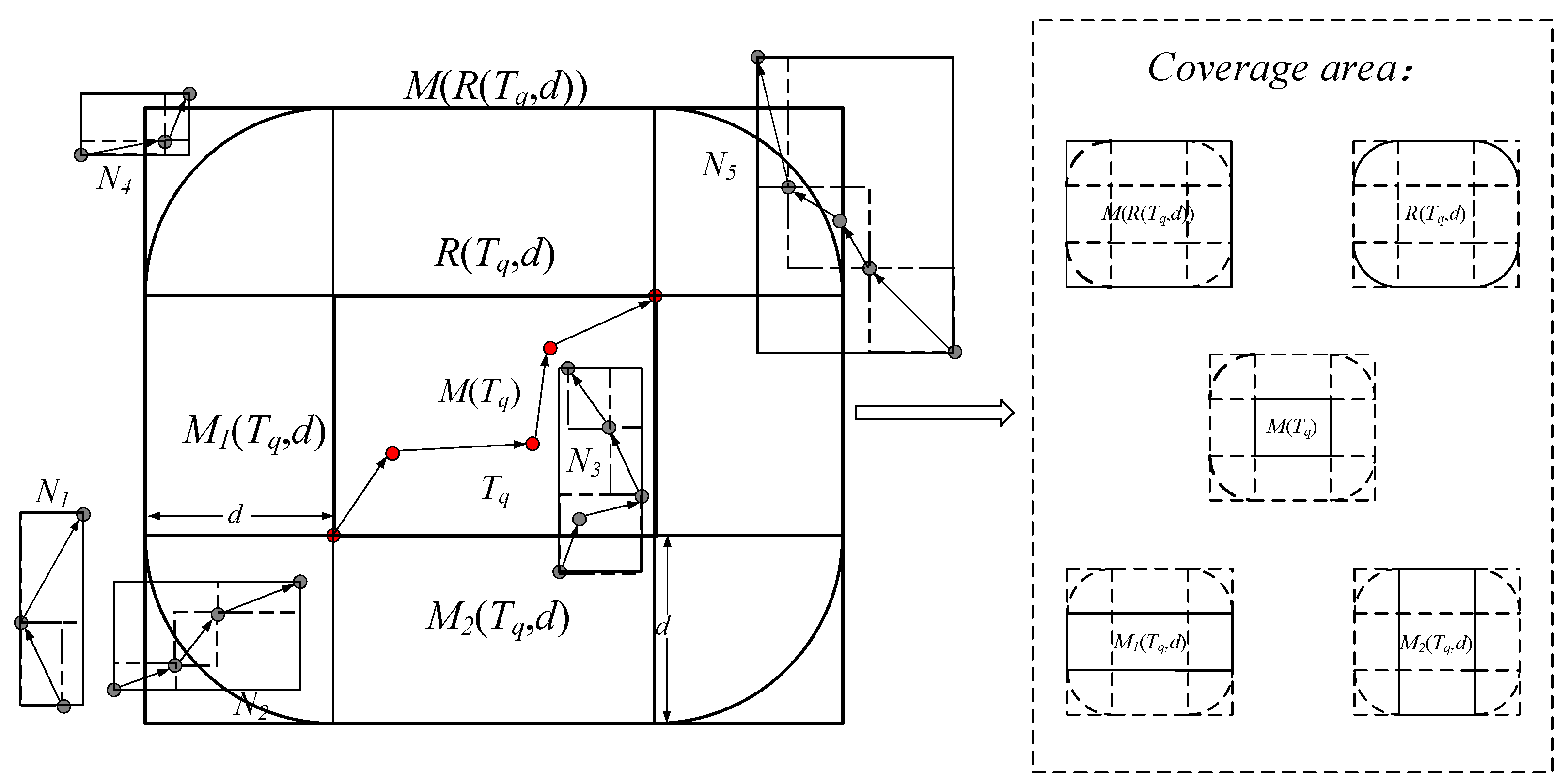
4.1. Extended MBR Overlap Based Pruning Strategy

Given a drtree node N_d, for N_d and query trajectory T_q, the basic pruning strategy consists of the following two steps:

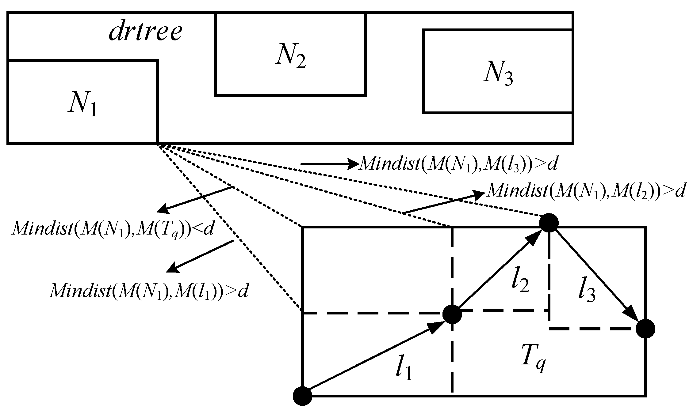
• Check whether the time interval of N_d overlaps with the time interval of T_q, if $TS(N_d)\cap TS(T_q)=\varnothing$, then N_d should be pruned.
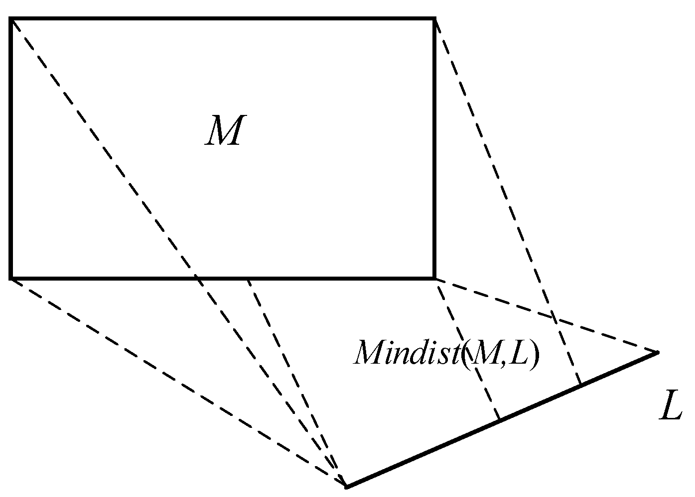
• Determine whether the Mindist between the MBR of N_d and the MBR of T_q is not greater than the distance threshold d, if $Mindist(M(N_d),M(T_q))>d$, then N_d should be pruned.

In the step (2) of the basic pruning strategy, although the Mindist-based method can effectively exclude the trajectory data that does not satisfy the query conditions, its calculation process is complicated and requires a lot of CPU time. When calculating the value of Mindist between $M(N_d)$ and $M(T_q)$, it first determines whether $M(N_d)$ is overlapped with $M(T_q)$, if so, then the value of Mindist is 0. Otherwise, it needs to calculate the minimum distance from any edge of $M(N_d)$ to $M(T_q)$, and chooses the minimum value as the value of Mindist, namely computing the MBR-to-MBR Mindist requires four times of Mindist calculations between a line segment and a rectangle. Moreover, a segment-to-rectangle Mindist calculation is subdivided into six times of distance calculations. As shown in Figure 3, when calculating the minimum distance between the line segment L and the rectangle M, it is necessary to calculate two Mindists from each vertex of L to M and four Mindists from each vertex of M to L, and then select the minimum value among them as the result. Hence, if $M(N_d)$ does not overlap with $M(T_q)$, 24 times of distance calculations are needed to get the value of Mindist between $M(N_d)$ and $M(T_q)$.

Obviously, the cost of calculating Mindist between two MBRs is expensive, and if the computational cost can be optimized, the query efficiency can be significantly improved. In the process of calculating Mindist, it can be noticed that the cost for checking whether two MBRs overlap is much smaller than the multiple distance calculation, which only needs to compare the spatial positional relationship between the MBR vertices. Suppose the spatial coordinates of the lower left and upper right corners of $M(N_d)$ are $(x_{d1},y_{d1})$ and $(x_{d2},y_{d2})$, the spatial coordinates of the lower left and upper right corners of $M(T_q)$ are $(x_{q1},y_{q1})$ and $(x_{q2},y_{q2})$, if the result of Discriminant (3) is true, then $M(N_d)$ is overlapped with $M(T_q)$. Taking advantage of the low overhead of overlapping calculation, we propose a pruning strategy based on extended MBR overlap to optimize the computational overhead.

$$!(((x_{d2}<x_{q1})\vee (y_{d1}>y_{q2}))\vee ((x_{q2}<x_{d1})\vee (y_{q1}>y_{d2}))).$$

(3)

First, we use the distance threshold d to extend the spatial range of $M(T_q)$. In the two-dimensional Euclidean space, we can get a coverage area $R(T_q,d)$ shaped as a rounded rectangle. It is easy to know that if the MBR of a drtree node overlaps with $R(T_q,d)$, then the Mindist between it and $M(T_q)$ is no larger than d. However, since the coverage area of $R(T_q,d)$ is not a rectangular area, determining whether $M(T_q)$ overlaps with $R(T_q,d)$ cannot be based only on the spatial positional relationship between the vertices, and additional calculations are required. With this in mind, we use the circumscribed rectangle $M(R(T_q,d))$ of $R(T_q,d)$ to approximate $R(T_q,d)$, if $M(N_d)$ does not overlap with $M(R(T_q,d))$, then it also does not overlap with $R(T_q,d)$. Hence, we summarize the Pruning strategy 1.

Pruning strategy 1.

Given a drtree node N_d and a query trajectory T_q, a distance threshold d, if $M(N_d)\cap M(R(T_q,d))=\varnothing$, then N_d must not contain data related to the query results, and it should be pruned.

Pruning strategy 1 does not involve complex calculations, so it can effectively reduce computational overhead. However, $M(R(T_q,d))$ increases the coverage area compared to $R(T_q,d)$, for such a drtree node whose MBR overlaps with $M(R(T_q,d))$ but does not overlap with $R(T_q,d)$, Pruning strategy 1 cannot prune it. For example, in Figure 4, Pruning strategy 1 cannot prune the node N₄. Therefore, the candidate set generated by using Pruning strategy 1 may contain more irrelevant candidates, which increases the processing overhead of refinement to some extent.

To overcome this problem, an intuitive method is to further check the drtree node that has passed the check of Pruning strategy 1 by calculating Mindist. However, as mentioned earlier, Mindist calculation requires a lot of CPU time and should be avoided during the pruning process. In this regard, we consider the property to be one or more rectangular areas that are fully covered by $R(T_q,d)$, if $M(N_d)$ overlaps with any of them, then $Mindist(M(N_d),M(T_q))\le d$. Further, to ensure the pruning effect, these rectangular areas should fully cover $M(T_q)$. Such a rectangular spatial area can be obtained by expanding the spatial range of each dimension of $M(T_q)$ by using d. Assuming that the coordinates of the lower left corner and the upper right corner of $M(T_q)$ are $(x_{q1},y_{q1})$ and $(x_{q2},y_{q2})$, respectively. Therefore, the coordinates of the lower left corner and upper right corner of $M_1(T_q,d)$ are $(x_{q1}-d,y_{q1})$ and $(x_{q2}+d,y_{q2})$, and the coordinates of the lower left corner and upper right corner of $M_2(T_q,d)$ are $(x_{q1},y_{q1}-d)$ and $(x_{q2},y_{q2}+d)$. It is easy to know that $M_1(T_q,d)$ and $M_2(T_q,d)$ are fully covered by $R(T_q,d)$, and $M(T_q)$ is fully covered by them. Hence, we obtain Pruning strategy 2.

Pruning strategy 2.

Given a query trajectory T_q, a distance threshold d, a drtree node N_d which has passed the check by Pruning strategy 1. If $(M(N_d)\cap M_1(T_q,d))\cup (M(N_d)\cap M_2(T_q,d))\ne \varnothing$, then the value of Mindist between M(N_d) and M(T_q) is not greater than d. Otherwise, we should calculate $Mindist(M(N_d),M(T_q))$ to determine whether pruning N_d.

For example, in Figure 4, nodes N₃ and N₅ overlap with $M_1(T_q,d)$, they need not be pruned, while nodes N₂ and N₄ do not overlap with $M_1(T_q,d)$ and $M_2(T_q,d)$, and it is necessary to further calculate the value of Mindist to decide whether pruning N₂ and N₄.

In summary, we name this method which combines Pruning strategy 1 and Pruning strategy 2 as Extended MBR overlap based pruning strategy (EMOB pruning strategy), Algorithm 1 gives its detailed flow. This algorithm is triggered when traversing each drtree node N_d. If the return value is true, then N_d should not be pruned. Otherwise, N_d should be pruned. The general flow of the algorithm is as follows:

• The algorithm first determines whether the time interval of N_d overlaps with the time interval of T_q. If there is overlap between the two, the algorithm will perform the next step, and return false otherwise (line 1 to 3).
• Whether $M(N_d)$ overlaps with $M(R(T_q,d))$ is checked. If any exist, the algorithm will continue to the next step. Otherwise, the false is returned (line 4 to 6).
• The algorithm judges whether $M(N_d)$ overlaps with $M_1(T_q,d)$ or $M_2(T_q,d)$. If no overlaps exist, the next step will be performed. Otherwise true is returned (line 7 to 9).
• Whether the value of $Mindist(M(N_d),M(T_q))$ is not larger than d is checked. The return value is true if $Mindist(M(N_d),M(T_q))\le d$. Otherwise false is returned (line 10 to 14).

Algorithm 1. EMOB Pruning Strategy

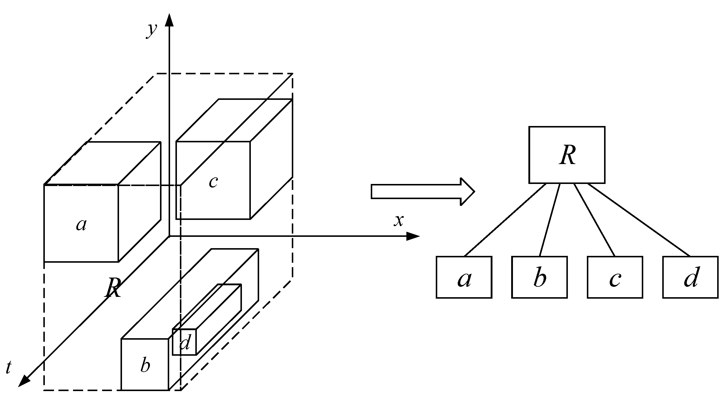
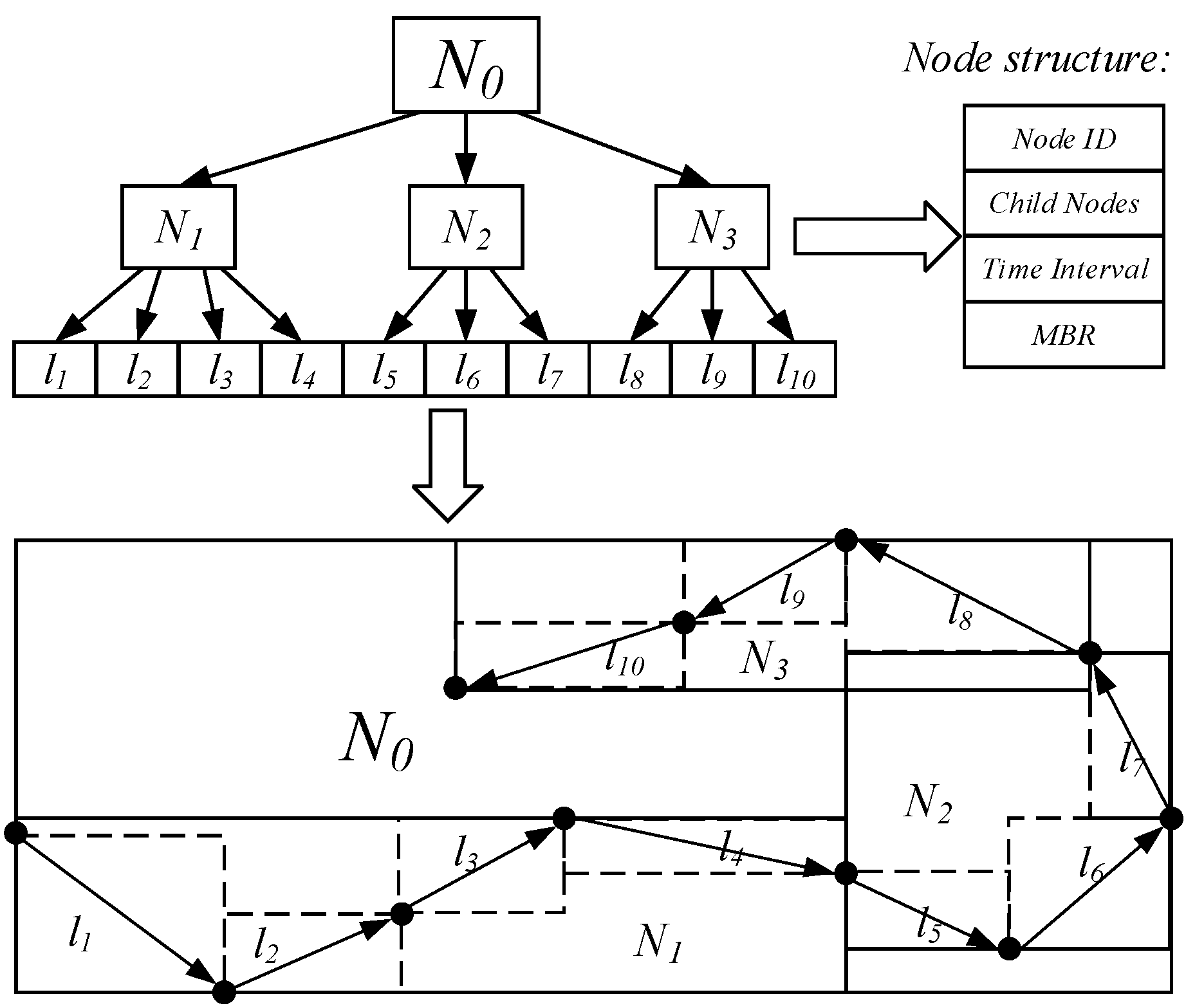
Input: Query trajectory Tq, drtree node Nd, Distance Threshold d; Output: The true value means retaining Nd, the false value means pruning Nd; 1 if$TS(N_d)\cap TS(T_q)=\varnothing$then 2  return false; 3 endif 4 if$M(N_d)\cap M(R(T_q,d))=\varnothing$then 5  return false; 6 endif 7 if$(M(N_d)\cap M_1(T_q,d))\cup (M(N_d)\cap M_2(T_q,d))\ne \varnothing$then 8  return true; 9 endif 10 if$Mindist(M(N_d),M(T_q))>d$then 11  return false; 12 else 13  return true; 14 endif

As with the basic pruning strategy, EMOB pruning strategy is also valid when any sub-trajectory of T_q is used as the pruning reference object. Hence, our method is suitable for higher precision pruning occasions. In Section 4.3, we will apply EMOB pruning strategy in the best-first traversal algorithm.

4.2. E3DR-Tree

Compared with the pruning method with taking the whole query trajectory as the pruning reference object, the pruning method with taking each trajectory segment of it as the reference one can obtain more accurate pruning results. This is because the invalid space of the MBRs which enclose the trajectory segments is less than that of the MBR which encloses the whole trajectory. For example, in Figure 5, the Mindist between the MBR of drtree node N₁ and $M(T_q)$ is smaller than d, but the Mindists between the MBR of the N₁ and the MBRs of the trajectory segment l₁ is greater than d. Therefore, N₁ does not satisfy the candidate requirement of l₁, and it is not necessary to calculate the distance between any trajectory segments contained in N₁ and l₁ in the refinement step.

Although the trajectory segment-based method can improve the pruning precision, in the pruning process, it is necessary to traverse the drtree once for each trajectory segment of T_q, resulting in a large increase in node traversal overhead. In order to reduce the node traversal overhead, we also organized all the trajectory segments contained in T_q by a spatiotemporal index called qrtree. In the pruning step, drtree and qrtree are traversed at the same time, this makes it possible to generate a precise pruning result without having to traverse the drtree multiple times, thus effectively reducing the overhead of traversing the nodes. The traversal algorithm will be discussed separately in Section 4.3, this section first describes the index structure used by qrtree.

Qrtree uses an index structure called the Extended 3DR-tree (E3DR-tree). An example of the structure of E3DR-tree is shown in Figure 6. The difference between E3DR-tree and the traditional 3DR-tree is shown in three aspects:

• Node selection condition. Whenever a trajectory segment is inserted, the node with the smallest change in the time interval is selected as the inserted node.
• Node split processing. When a node needs to be split, while balancing the number of child nodes included in the new nodes, it is also necessary to ensure that the time intervals of new nodes have no overlap.
• The child nodes (or trajectory segments) of a node are sorted in the ascending order of the start timestamp of the corresponding time interval.

Although the construction of E3DR-tree does not consider the spatial factor directly, for the trajectory data of the same moving object, the trajectory segments that are close in time are usually close in space, so E3DR-tree still has a strong spatial distinguishing ability. Moreover, E3DR-tree ensures that the trajectory segments can be processed in chronological order during traversal, which is consistent with their order in the trajectory so that the overhead of the subsequent sorting processing can be effectively reduced.

4.3. Best-First Traversal Algorithm

We designed a best-first traversal algorithm that traverses drtree and qrtree simultaneously to handle the pruning process. Compared to the pruning method that traverses drtree alone, it can generate an accurate result with accessing fewer nodes. Its basic principle is to select the accessed objects of the next iteration according to the heights of the accessed drtree node and the qrtree node. As the number of iterations increases, the pruning precision continues to rise, a set of candidate trajectory segments is eventually generated for each trajectory segment of T_q.

To support the best-first traversal algorithm, we use a first priority queue (FirstPQ) and multiple secondary priority queues (SecPQ) to record the intermediate results during the traversal process [18]. FirstPQ is used to control the traversal order of the qrtree nodes, and SecPQ is used to control the traversal of the drtree nodes. First, the data structures of FirstPQ entry (F-entry) and SecPQ entry (S-entry) are introduced.

Definition 3.

Attributes of each F-entry $(N_q,h_q,t_q,SPQ)$ are described as follows:

(1)

Node N_q—a qrtree node, which can be an index node or a trajectory segment;

(2)

Height h_q—the height from N_q to the trajectory segment layer of qrtree. if $h_q=0$, then N_q is a trajectory segment. In addition, the F-entries in a FirstPQ are sorted by h_q value (largest to smallest).

(3)

Timestamp t_q—the starting timestamp of the time interval of N_q. In addition, t_q is the secondary keyword for sorting F-entries, when two F-entries have the same h_q value, they are sorted by t_q value (smallest to largest).

(4)

SecPQ SPQ—a SecPQ that records the qrtree nodes which pass the pruning check with N_q.

Definition 4.

Attributes of each S-entry $(N_d,h_d,t_d)$ are described as follows:

(1)

Node N_d—a drtree node, which can be an index node or a trajectory segment;

(2)

Height h_d—the height from N_d to the trajectory segment layer of drtree. if $h_d=0$, then N_d is a trajectory segment. In addition, the S-entries in a SecPQ are sorted by h_d value (largest to smallest).

(3)

Timestamp t_d—the starting timestamp of the time interval of N_d. In addition, t_d is the secondary keyword for sorting S-entries, when two S-entries have the same h_d value, they are sorted by t_d value (smallest to largest).

Algorithm 2 gives its detailed flow of the best first traversal algorithm, it is divided into two steps of initialization (lines 1 to 8) and iteration (lines 9 to 19) and using a collection Ps to collect all pruning results.

In the initialization step, an E3DR tree qrtree is first created for the query trajectory T_q (line 1). A SecPQ SPQ and a FirstPQ FPQ are then initialized (lines 2 to 3). Next, the root nodes of qrtree and drtree are obtained, and the pruning check is performed. If the root node of drtree is not be pruned, an S-entry and an F-entry are created and inserted in SPQ and FPQ, respectively. Otherwise, the algorithm ends (lines 4 to 8).

For each iteration of the while loop, the first F-entry fe₁ is dequeued from FPQ, and the head S-entry se₁ of the fe₁.SPQ is also checked without dequeuing (lines 10 to 11). Based on the values of fe₁.h_q and se.h_d, a decision is made whether to traverse qrtree, to traverse drtree or to add a pruning result to Ps, the processing of the three cases are as follows:

• Case 1 (At least one of fe₁.h_q and se₁.h_d is not 0, and $f{e}_1.h_q\ge s{e}_1.h_d$_-): The child nodes of fe₁.N_q are traversed by the function TRA-Q(FPQ, fe₁, d), and when each child node is accessed, the pruning check is performed for the drtree node of each S-entry in fe₁.SPQ (lines 12 to 13). The pseudo code of the function TRA-Q(FPQ, fe₁, d) is shown in Algorithm 3.
• Case 2 (At least one of fe₁.h_q and se₁.h_d is not 0, and $f{e}_1.h_q<s{e}_1.h_d$): The child nodes of se₁.N_d are traversed by the function TRA-D(FPQ, fe₁, d), and the pruning check is performed when each child node is accessed (lines 14 to 15). The pseudo code of the function TRA-D(FPQ, fe₁, d) is shown in Algorithm 4.
• Case 3 (Both of fe₁.h_q and se₁.h_d are 0): Namely both of fe₁.N_q and se₁.N_d are the trajectory segments. Moreover, according to the ordering rule of SecPQ, the drtree node of any S-entry in fe₁.SPQ is also a trajectory segment and is a candidate of fe₁.N_q. Therefore, fe₁ can be regarded as a pruning result and added to Ps (line 16 to 17).

Algorithm 2. Best-First Traversal Algorithm

Input: Query Trajectory Tq, distance threshold d, drtree; Output: Pruning results Ps; 1 qrtree←Create an E3DR-tree for trajectory Tq; 2 SPQ←initialize an instance of SecPQ; 3 FPQ←initialize an instance of FirstPQ; 4 Nd←Root(drtree); 5 Nq←Root(qrtree); 6 if EMOB(Nd, Nq, d)=true then 7  SPQ.enqueue((Nd, H(Nd), TS(Nd))); 8  FPQ.enqueue((Nq, H(Nq), TS(Nq), SPQ)); 9  while $FPQ\ne \varnothing$ do 10   fe1←FPQ.dequeue(); 11   se1←fe1.SPQ.getFirst(); 12   if $(f{e}_1.h_q\ne 0\vee s{e}_1.h_d\ne 0)\wedge (f{e}_1.h_q\ge s{e}_1.h_d)$ then 13    TRA-Q(FPQ, fe1, d); 14   else if $(f{e}_1.h_q\ne 0\vee s{e}_1.h_d\ne 0)\wedge (f{e}_1.h_q<s{e}_1.h_d)$ then 15    TRA-D(FPQ, fe1, d); 16   else if $f{e}_1.h_q=0\wedge s{e}_1.h_d=0$ then 17    Ps.add(fe1); 18   endif 19  endwhile 20 endif 21 returnPs;

In the function TRA-Q(FPQ, fe₁, d), for each child node C_q of the node fe₁.N_q, the following processing is performed:

• Initialize a SecPQ CSPQ (line 2);
• Loop read each S-entry of fe₁.SPQ (without dequeuing), let cse be the current read S-entry if cse.N_d is not pruned, then cse is inserted into CSPQ (lines 3 to 7).
• Create a new F-entry for C_q by using the relevant parameters and insert it into FPQ (line 8).

Algorithm 3. TRA-Q(FPQ, fe1, d)

Input: FirstPQ FPQ, F-entry fe1, distance threshold d; Output: Null; 1 for each child node Cq of fe1.Nq do 2  CSPQ←initialize an instance of SecPQ; 3  for each entry cse of fe1.SPQ do 4   if EMOB(cse.Nd, Cq, d)=true then 5    CSPQ.enqueue(cse); 6   endif 7  endfor 8  FPQ.enqueue((Cq, H(Cq), TS(Cq), CSPQ)); 9 endfor

The process of the function TRA-D (FPQ, fe₁, d) is as follows:

• Dequeue the head S-entry se₁ from fe₁.SPQ (line);
• Traverse the child nodes of se₁.N_d, and perform the pruning check for each child node C_d, if C_d is not pruned, then an S-entry is created for C_d and inserted into fe₁.SPQ (line 2 to 6);
• Insert fe₁ into FPQ again (line 7).

Algorithm 4. TRA-D(FPQ, fe1, d)

Input: FirstPQ FPQ, F-entry fe1, distance threshold d; Output: Null; 1 se1←fe1.SPQ.dequeue(); 2 for each child node Cd of se1.Nd do 3  if EMOB (Cd, fe1.Nq, d)=true then 4   fe1.SPQ.enqueue(Cd, H(Cd), TS(Cd)); 5  endif 6 endfor 7 FPQ.enqueue(fe1);

The best-first traversal algorithm ends when there are no F-entries in FPQ. According to the F- entry structure, each entry of Ps records a query trajectory segment of T_q and a set of candidate trajectory segments, and the entries of Ps are sorted based on the chronological order of the query trajectory segment, so in the refinement step, the entries of Ps will be processed naturally in chronological order, thereby effectively reducing the processing overhead of sorting. Compared with the method of pruning drtree nodes with taking the whole query trajectory as the pruning reference object, the best priority traversal algorithm can generate more accurate candidate results and reduce the overhead required for the refinement step. In addition, because our method adopts the strategy of traversing drtree and qrtree at the same time, it ensures that the drtree is not traversed multiple times in the case of obtaining a high-precision pruning results, so the cost of accessing the index nodes is greatly reduced.

After the pruning step is finished, the candidate trajectory segments need to be refined to obtain the final results. Since the focus of our study is pruning optimization, the refinement step is only briefly explained here, and the detailed process of the refinement step of the historical continuous query can be found in the literature [6]. In the pruning result Ps, for each trajectory segment l_q of T_q, assume that one of its candidate trajectory segments is l_d. First, l_d is interpolated to obtain the time interval ti_q that overlaps with that of l_q. Then the distance between l_d and l_q at any time instance in ti_q is calculated, the square of this distance is a quadratic expression with time as the parameter. Next, the distance threshold d is brought into the expression to obtain a quadratic equation inequality, this inequality is solved to obtain a time interval ti_c where the distance between l_d and l_q is less than d. If ti_q overlaps with ti_c (naming the overlap time Interval as ti_o), then the moving object l_d.oid is a query result of ti_o. After all the data of Ps is processed, all the query results are returned to the user, and the query ends.

4.4. Performance Analysis

The time complexity of the best-first traversal algorithm comes from the processes of creating the E3DR-tree and iterative searching. Suppose that the query trajectory T_q and the moving object database D contain respectively n and m trajectory segments. First, in the aspect of creating the E3DR- tree, since the E3DR-tree is created in the same way as the traditional R-tree, the running time of creating it is O(nlogn). Second, in the aspect of iterative searching, all candidate trajectory segments are concentrated on just one leaf node of the drtree in the best case, so the time complexity is O(n+logm). Conversely, in the worst case, each trajectory segment in T_q needs to match each trajectory segment in D, it takes O(mn) rounds of computation. Certainly, it is difficult to achieve the theoretical worst-case complexity when actually performing iterative searching. In summary, the total time complexity of the best-first traversal algorithm is O(nlogn+logm) to O(nlogn+mn).

Figure 7 shows an example of the pruning process of THC query, where T_q contains six trajectory segments, each trajectory in D contains four trajectory segments, and the distance threshold d is one. The maximum number of children of a node in the 3DR-tree that indexes T_q or D is three. Considering that there are not many trajectory segments in the example, we do not consider the time attribute, and only performed pruning based on the spatial distance.

The best first traversal algorithm (shorted as BFT) takes a total of 105 pruning checks to get the pruning results, in which the number of pruning is 100 times by checking the overlap between the MBRs, and the number of pruning is only five times by checking the Mindist. As a comparison, the pruning method proposed in literature [10] that takes each segment of the query trajectory as a reference object (shorted as TDS) takes 114 pruning checks, while the pruning method proposed in literature [12] (shorted as CDQLTD) that regards the whole query trajectory as the pruning reference takes only 31 pruning checks. From the pruning results shown in

Table 2. Comparison of pruning results.

Trajectory Segment	Candidate Quantity (BFT)	Candidate Quantity (TDS)	Candidate Quantity (CDQLTD)
l1	0	1	15
l2	2	2	15
l3	8	10	15
l4	10	11	15
l5	4	4	15
l6	6	7	15

, benefiting from the segment-based pruning way, the pruning results of TDS and BFT are closer to the final results than that of CDQLTD. Moreover, compared to TDS, due to the pruning strategy that combines MBR overlap and Mindist calculation, the pruning accuracy achieved by BFT is more than that of TDS.

5. Experiment

5.1. Experimental Set Up

In order to verify the effectiveness of our pruning optimization method, we implemented it in Java and verified in the Linux environment. For the experiment, a PC (Intel Xeon E5-2620 V2, 16GB memory, 2TB disk) running Ubuntu 16.04 64-bit was used.

The experiments used the global AIS (Automatic Identification System) [19] data from 1 July to 5 July 2012 as the data source, in which each AIS message was regarded as a spatial location of a moving object at a timestamp. We randomly extracted some data from the data source to form five datasets. The statistical information is shown in

Table 3. Statistics of Datasets.

Name	No. of Moving Objects	No. of AIS Messages
AIS01	73,490	10,000,000
AIS02	95,732	20,000,000
AIS03	110,566	40,000,000
AIS04	136,932	80,000,000
AIS05	152,807	160,000,000

. When constructing a 3DR-tree for a dataset during the experiment, it was considered that the motion track between the spatial positions with a long time interval may be significantly different from the real motion track, according to the maximum transmission time interval of the AIS message, we made the following provisions: If an AIS message had an adjacent message within six minutes of the time interval, the motion track between the spatial positions of the two messages was taken as a trajectory segment. Otherwise, it was regarded as a special trajectory segment with the same start time and end time. We evaluated the performance of BFT with TDS [10] and CDQLTD [12]. The query performances were evaluated under different data scales, different time ranges and different distance thresholds. The evaluated metrics included the following four aspects:

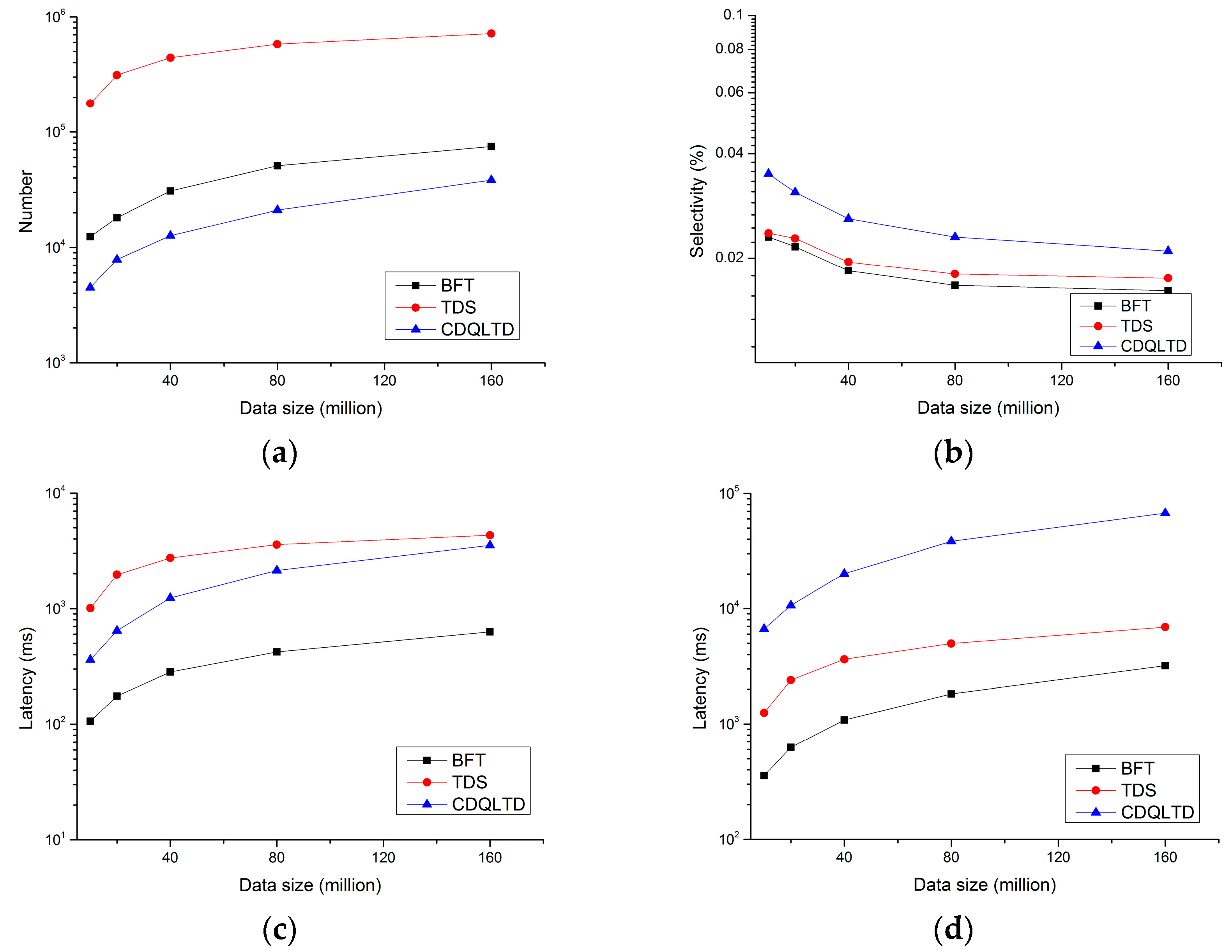
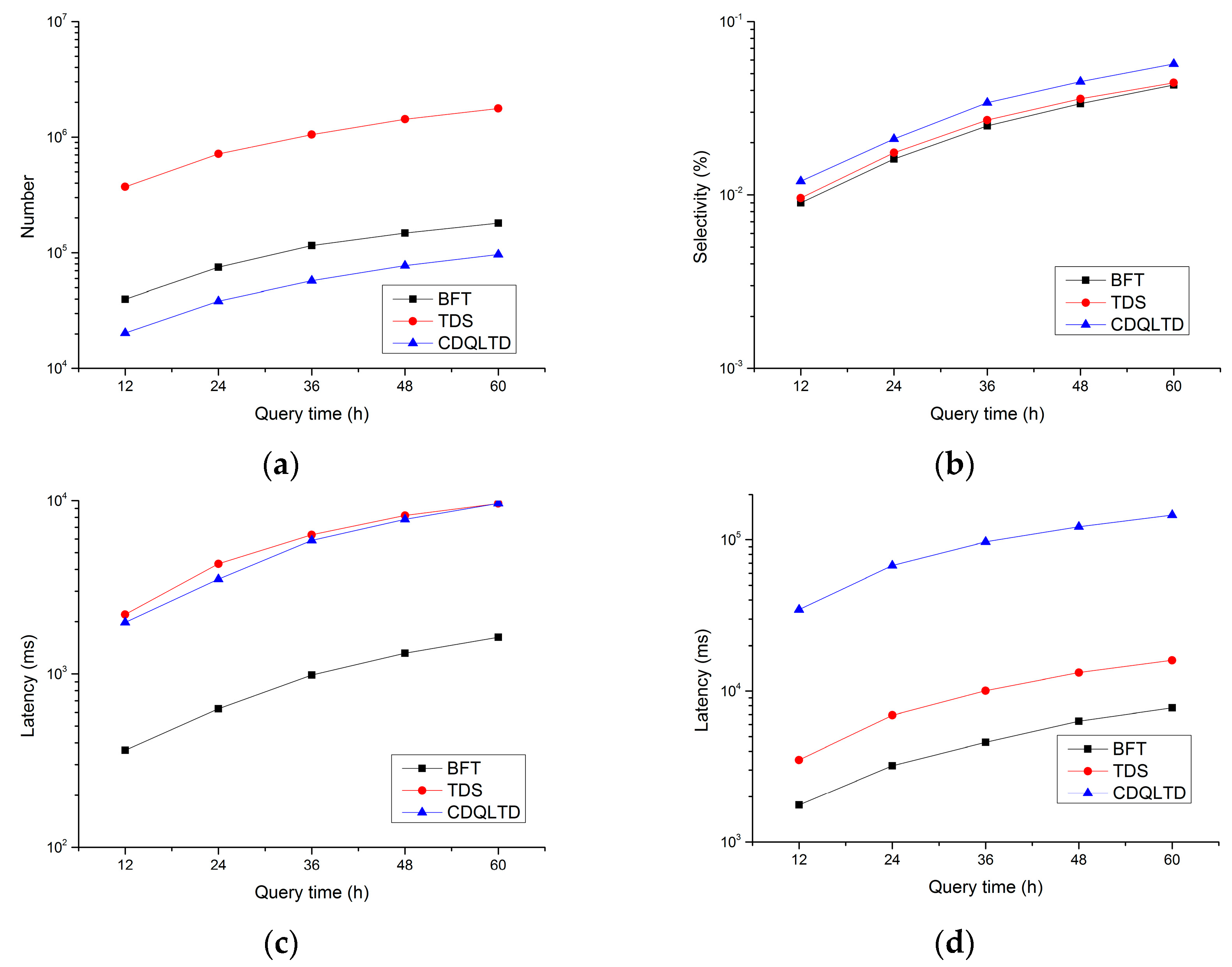
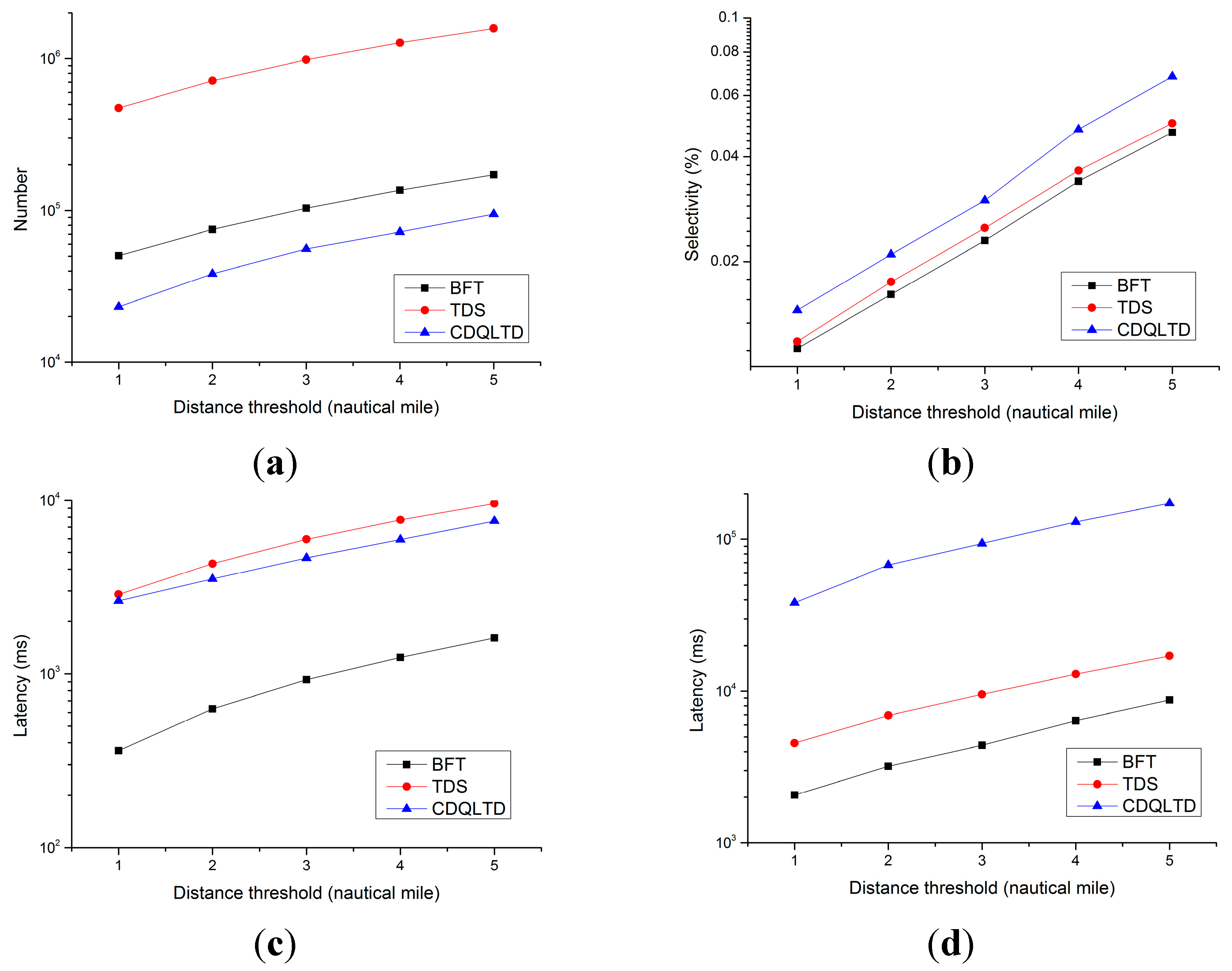
• Number of the accessed nodes: The sum of the number of index nodes and the number of trajectory segments checked during pruning;
• Selectivity: The ratio of the number of candidate trajectory segments obtained by pruning to the number of trajectory segments contained in the dataset;
• Pruning Latency: The execution time of the pruning step during a query;
• Query Latency: The execution time of a query.

For each experiment, we performed 50 queries, and used the average as the experiment result. By default, we used AIS05 as the experimental dataset, 24 h as the query time range, and two nautical miles as the distance threshold.

5.2. Performance of Different Data Scales

In this part of the experiments, datasets AIS01, AIS02, AIS03, AIS04, and AIS05 were used as experimental data to evaluate the query performance of the three methods under different scales, as shown in Figure 8.

It can be seen from Figure 8a,b that as the data scale increases, the number of accessed nodes increases in the pruning step. However, the increase rate of the pruning results is smaller than the change of data scales, so the selectivity is gradually decreasing. Among the three methods, CDQLTD has the fewest number of the accessed nodes, because it uses a single MBR of the whole query trajectory as the pruning reference, and the spatiotemporal index of the dataset only needs to be traversed once. However, CDQLTD has the lowest pruning precision, and the pruning results contain some irrelevant data, so CDQLTD has the worst selectivity. While TDS uses each trajectory segment of the query trajectory as the reference, it is necessary to repeatedly traverse the spatiotemporal index of the dataset, and the number of the accessed nodes is one order of magnitude larger than the two methods. However, it also benefits from the segment-based pruning way, the pruning results of TDS is closer to the final query results, so its selectivity performance is better than that of CDQLTD. BFT also uses each query trajectory segment as the pruning reference, but thanks to the E3DR-tree structure and the best-first traversal algorithm, the number of the accessed node is much smaller than that of TDS. Moreover, the pruning strategy adopted by BFT combines MBR overlap and Mindist calculation, so the selectivity performance of BFT is better than that of TDS which only consider MBR overlap.

Figure 8c shows the performance of pruning latency. Since BFT accesses fewer nodes and its pruning strategy based on extended MBR overlap effectively reduce the time overhead of a single pruning check, so BFT takes less time than the two methods. Although CDQLTD visits the fewest nodes when pruning, the calculation process of pruning check based on Mindist is complex and time-consuming, resulting in a large time overhead for the entire pruning process. TDS has the lowest time-consuming pruning check method, but the number of the accessed nodes is much more than the two methods, resulting in the most time-consuming pruning.

The performance of query latency is shown in Figure 8d, where BFT performs best, not only because BFT takes the least time to complete the pruning step, but also generates the highest precision of pruning results, so the process of refinement also takes the least time. The pruning results of CDQLTD have the lowest precision, which makes it necessary to spend a lot of time on refinement processing, the time difference between it and the two methods will be further amplified as the data scale increases.

5.3. Performance of Different Time Ranges

Figure 9 shows the query performance of the three different methods at different time ranges. It can be seen from Figure 9a that as the query time range increases, the number of candidates involved also increases, and all three methods need to access more nodes to obtain candidates. Figure 9b shows that the change in selectivity is proportional to the change in the time range, this is because the increase in the number of candidate segments will naturally increase the selectivity when the data size is constant. As shown in Figure 9c,d, since all three methods require more time to generate and process the candidate segments, their pruning latency and query latency increase with the increase of time range. Among the three methods, BFT has the best query performance. In all cases, BFT takes less than eight seconds to complete the query process, while the time spent by CDQLTD gradually increases from 34 s to 134 s. The reason for this difference in performance has been explained in Section 5.2, it will not be described in detail here.

5.4. Performance of Different Distance Thresholds

This part of the experiments evaluated the query performance of different distance thresholds, as shown in Figure 10. As the distance threshold increases, the query spatial range of query increases, and the increased speed shows an increasing trend. It causes more index nodes and trajectory segments to be accessed and checked, and the pruning results contain more candidates. As shown in Figure 10a,b, the growth rate of the number of accessed nodes, and that of selectivity will also increase. Naturally, when the distance threshold is increased from one nautical mile to five nautical miles. It can be seen from Figure 10c,d that the pruning latency and query latency of the three methods also increases. Among them, the performance of BFT is still better than that of the other two. In terms of pruning latency, it takes less than one-fifth of the two methods. In terms of query latency, it takes less than half of that of TDS, and is an order of magnitude smaller than that of CDQLTD.

5.5. Summary of the Experiments

In order to measure the performance of our pruning method, we conducted the above experimental study based on a real dataset. Regarding the historical continuous queries, it has been shown that the best-first traversal algorithm always has better performance of selectivity rate and query latency compared with the other two methods in all cases. This is because the pruning accuracy and the number of accessed nodes are considered comprehensively in our method. Moreover, we demonstrated that our improvement over the pruning strategy can sufficiently increase the performance of the proposed algorithms, compared with CDQLTD method, it achieves less pruning latency in the case of accessing more nodes.

6. Conclusions

We studied a specific sub-domain of the continuous queries of moving objects, namely the pruning optimization of historical continuous queries based on a threshold. First, we optimized the processing overhead of a single pruning check using a pruning strategy based on extended MBR overlap. Secondly, a 3DR-tree extension structure called E3DR-tree was proposed for traversing the query trajectory, and based on this, the best-first traversal algorithm was introduced, so that the accurate pruning results could be obtained with accessing as few nodes as possible. Finally, a large number of experimental results verify the effectiveness of our method. In the future work, we plan to apply this method to the distributed environment, and combine it with a distributed index, to further improve the query performance based on parallelization techniques. Moreover, we will improve this method to solve another sub-problem of historical continuous query—k-nearest history continuous query.

References

1. Zhang, Z.; Jin, C.; Mao, J.; Yang, X.; Zhou, A. TrajSpark: A Scalable and Efficient In-Memory Management System for Big Trajectory Data. In Proceedings of the Asia-Pacific Web (APWeb) and Web-Age Information Management (WAIM) Joint Conference on Web and Big Data, Beijing, China, 7–9 July 2017. [Google Scholar]
2. Salmon, L.; Ray, C. Design principles of a stream-based framework for mobility analysis. GeoInformatica 2017, 21, 237–261. [Google Scholar] [CrossRef]
3. Nutanong, S.; Ali, M.E.; Tanin, E.; Mouratidis, K. Dynamic Nearest Neighbor Queries in Euclidean Space. Encycl. GIS 2015, 1–7. [Google Scholar]
4. Trajcevski, G.; Tamassia, R.; Cruz, I.F.; Scheuermann, P.; Hartglass, D.; Zamierowski, C. Ranking continuous nearest neighbors for uncertain trajectories. VLDB J. 2011, 20, 767–791. [Google Scholar] [CrossRef]
5. Theodoridis, Y.; Vazirgiannis, M.; Sellis, T. Spatio-temporal indexing for large multimedia applications. In Proceedings of the Third IEEE International Conference on Multimedia Computing and Systems, Hiroshima, Japan, 17–23 June 1996. [Google Scholar]
6. Frentzos, E.; Gratsias, K.; Pelekis, N.; Theodoridis, Y. Algorithms for nearest neighbor search on moving object trajectories. Geoinformatica 2007, 11, 159–193. [Google Scholar] [CrossRef]
7. Papadias, D.; Zhang, J.; Mamoulis, N.; Tao, Y. Query processing in spatial network databases. In Proceedings of the 29th International Conference on Very Large Data Bases, Berlin, Germany, 9–12 September 2003. [Google Scholar]
8. Pfoser, D.; Jensen, C.S.; Theodoridis, Y. Novel Approaches in Query Processing for Moving Object Trajectories. In Proceedings of the 26th International Conference on Very Large Data Bases, Cairo, Egypt, 10–14 September 2000. [Google Scholar]
9. Güting, R.H.; Behr, T.; Xu, J. Efficient k-nearest neighbor search on moving object trajectories. VLDB J. 2010, 19, 687–714. [Google Scholar]
10. Gowanlock, M.; Casanova, H. In-memory distance threshold queries on moving object trajectories. In Proceedings of the Sixth International Conference on Advances in Databases, Knowledge, and Data Applications, Chamonix, France, 20–25 April 2014. [Google Scholar]
11. Dagum, L.; Menon, R. OpenMP: An industry-standard API for shared-memory programming. CiSE 1998, 1, 46–55. [Google Scholar] [CrossRef]
12. Huorong, H.; Jianqiu, X.; Xiaolin, Q. Continuous Distance Queries over Large Trajectory Data. J. Chin. Comput. Syst. 2017, 38, 2505–2510. (In Chinese) [Google Scholar]
13. Chakka, V.P.; Everspaugh, A.; Patel, J.M. Indexing large trajectory data sets with SETI. CIDR 2003, 75, 76. [Google Scholar]
14. Gowanlock, M.; Casanova, H. Distance threshold similarity searches on spatiotemporal trajectories using GPGPU. In Proceedings of the 2014 21st International Conference on High Performance Computing (HiPC), Goa, India, 17–20 December 2014. [Google Scholar]
15. Gowanlock, M.; Casanova, H. Indexing of spatiotemporal trajectories for efficient distance threshold similarity searches on the GPU. In Proceedings of the 2015 IEEE International Parallel and Distributed Processing Symposium, Hyderabad, India, 25–29 May 2015. [Google Scholar]
16. Gowanlock, M.; Casanova, H. Distance threshold similarity searches: Efficient trajectory indexing on the GPU. IEEE Trans. Parallel Distrib. Syst. 2016, 27, 2533–2545. [Google Scholar] [CrossRef]
17. Mahmood, A.R.; Punni, S.; Aref, W.G. Spatio-temporal access methods: A survey (2010–2017). GeoInformatica 2019, 23, 1–36. [Google Scholar] [CrossRef]
18. Nutanong, S.; Jacox, E.H.; Samet, H. An Incremental Hausdorff Distance Calculation Algorithm. Proc. VLDB Endow. 2011, 4, 506–517. [Google Scholar] [CrossRef]
19. Harati-Mokhtari, A.; Wall, A.; Brooks, P.; Wang, J. Automatic Identification System (AIS): Data reliability and human error implications. J. Navig. 2007, 60, 373–389. [Google Scholar] [CrossRef]
Figure 1. Example of threshold-based historical continuous (THC) query.
Algorithms 12 00107 g001
Figure 2. The example of 3DR-tree.
Algorithms 12 00107 g002
Figure 3. The Mindist between a line segment and a rectangle.
Algorithms 12 00107 g003
Figure 4. Example of extended MBR overlap based pruning strategy.
Algorithms 12 00107 g004
Figure 5. Example of Mindists of different data granularities.
Algorithms 12 00107 g005
Figure 6. Example of E3DR-tree.
Algorithms 12 00107 g006
Figure 7. Example of the pruning process of THC query.
Algorithms 12 00107 g007
Figure 8. Performance of different scales: (a) Number of the accessed nodes, (b) selectivity, (c) pruning latency, (d) query latency.
Algorithms 12 00107 g008
Figure 9. Performance of different time ranges: (a) Number of the accessed nodes, (b) selectivity, (c) pruning latency, (d) query latency.
Algorithms 12 00107 g009
Figure 10. Performance of different distance thresholds: (a) Number of the accessed nodes, (b) selectivity, (c) pruning latency, (d) query latency.
Algorithms 12 00107 g010