Forecasting Economy-Related Data Utilizing Weight-Constrained Recurrent Neural Networks

Abstract

During the last few decades, machine learning has constituted a significant tool in extracting useful knowledge from economic data for assisting decision-making. In this work, we evaluate the performance of weight-constrained recurrent neural networks in forecasting economic classification problems. These networks are efficiently trained with a recently-proposed training algorithm, which has two major advantages. Firstly, it exploits the numerical efficiency and very low memory requirements of the limited memory BFGS matrices; secondly, it utilizes a gradient-projection strategy for handling the bounds on the weights. The reported numerical experiments present the classification accuracy of the proposed model, providing empirical evidence that the application of the bounds on the weights of the recurrent neural network provides more stable and reliable learning.

1. Introduction

The rapid advances in digital technologies, as well as the vigorous development of the Internet and the significant storage capabilities of electronic media have enabled economic research centers to accumulate and store large repositories of data. This enormous amount of valuable data yields information of various economic activities such as credit history of bank customers, stock market prices and movement, companies and business funds’ sales records, and other statistics. It is a fundamental need for business, companies, and banks to extract useful knowledge from these data. This knowledge constitutes a key element for better decision-making in the increasing market volatility and competition.

Economic data mining constitutes an essential process where intelligent methods are applied to extract data patterns from economic databases. This research area has rapidly grown and gained popularity in the modern economic era due to its potential to assist managerial decision-making. During the last two decades, researchers and financial managers have begun to analyze economic data utilizing machine learning and data mining techniques for supporting hard policy decisions (see [1,2,3,4] and the references therein). As a result, the area of economic analysis has been dramatically changed from a rather qualitative science to a more quantitative science, which is also based on knowledge extraction from databases. Nevertheless, economic data are usually imbalanced and are usually characterized by complex dimensionality and enormous noise, hindering their analysis and modeling. Therefore, the process of leveraging these data constitutes an attractive and challenging task for many experts, which often requires huge efforts.

Artificial Neural Networks (ANN) have been established as some of the most dominant machine learning algorithms for extracting useful knowledge; thus their value has been demonstrated across an impressive spectrum of applications [5,6,7,8]. Due to their excellent capability of self-learning and self-adapting, they are very appealing to deal with economic and financial problems with poorly-defined system models, noisy data, and strong presence of nonlinear effects. In the literature, several neural network architectures have been proposed [9]. Recurrent Neural Networks (RNNs) constitute a class of neural networks that are well known for their power to memorize time dependencies and model nonlinear systems.In contrast to the classical feed-forward neural networks in which all the inputs and outputs are independent of each other, RNNs allow previous outputs to be used as inputs while having hidden states. Their main advantages are their ability to deal with time-varying input and output through their own natural temporal operation [10,11,12].

Mathematically, the problem of efficiently training an RNN can be formulated as the minimization of an error function $E\left(w\right)$, which depends on the connection weights w of the network. Recently, Livieris [13] proposed a new approach for improving the generalization ability of neural networks, by applying additional conditions on the weights in the form of bound constraints, during the training process. The motivation behind this approach focuses on defining the weights of the trained network in a more uniform way in order for all inputs and neurons of the network to be efficiently explored and exploited. Therefore, the problem of training a neural network is reformulated as a constrained optimization problem, namely:

$$min\left\{E\right(w):w\in \mathcal{B}\},$$

(1)

with:

$$\mathcal{B}=\{w\in {\mathbb{R}}^n:l\le w\le u\},$$

(2)

where $l\in {\mathbb{R}}^n$ and $u\in {\mathbb{R}}^n$ denote the lower and upper bounds on the weights, respectively. Moreover, to evaluate the efficacy and the efficiency of this approach, Livieris proposed a new weight-constrained neural network training algorithm. The proposed algorithm exploits the numerical efficiency and very low memory requirements of the limited memory BFGS matrices together with a gradient-projection strategy for handling the bounds on the weights.

In this work, we examine and evaluate the performance of weight-constrained recurrent neural networks for the classification of economic data. To this end, we conducted a series of experiments using three famous economic classification problems, the bank marketing problem, the German credit approval problem, and the banknote authentication dataset. Our numerical experiments demonstrate that the classification efficiency of the proposed algorithm outperforms classical neural network training algorithms, providing empirical evidence that it provides more stable, efficient, and reliable learning.

The remainder of this paper is organized as follows: Section 2 briefly discusses recent studies concerning the application of machine learning in economic data. Section 3 presents the weight-constrained recurrent neural network training algorithm. Section 4 presents the numerical experiments utilizing the performance profiles of Dolan and Morè [14]. Finally, Section 5 presents the conclusions and our proposals for future research.

Notations. Throughout this paper, the gradient of the error function is indicated by $\nabla E\left(w\right)$, and the vectors $s_k=w_{k+1}-w_k$ and $y_k=\nabla E\left(w_{k+1}\right)-\nabla E\left(w_k\right)$ represent the evolutions of the current point and of the error function gradient between two successive iterations.

2. Related Work

Research on the predictability of economic data has a long history in economics; thus economic data mining systems have gained popularity during the last two decades. The main reason for the increasing popularity of these systems is their ability to support economic decision-making considerations such as information acquisition and decision-making error costs. A number of rewarding studies have been carried out in recent years, and some useful outcomes are briefly presented below.

Chang et al. [1] proposed a novel classifier based on the Artificial Immune Network (AINE) to evaluate the applicants’ credit scores. Additionally, they conducted a variety of experiments, utilizing two real-world datasets of the banking industries to explore the effectiveness of their proposed model. The presented experimental results demonstrated that the AINE-based classifier outperformed state-of-the-art classifiers, in terms of prediction accuracy. Furthermore, the authors claimed that the proposed model can provide the credit card issuer with accurate and valuable information of credit scoring analysis to avoid making incorrect decisions.

Moro et al. [2] proposed a personal and intelligent decision support system that utilizes a data mining approach for the selection of bank telemarketing clients. Their primary goal was to model the success of subscribing to a long-term deposit using attributes that were known before the telemarketing call was executed. For this purpose, they utilized a large dataset of 150 features related to bank client, product, and social-economic attributes. In the modeling phase of their proposed framework, a semi-automatic feature selection was explored, which resulted in selecting a reduced set of 22 features. In the sequel, they evaluated the classification performance of various machine learning algorithms. Their experimental results revealed that ANN demonstrated the highest classification accuracy.

Tkavc et al. [3] provided an extensive review of neural networks applications on several economic and business classification problems. Their investigation revealed that most of the research was aimed at financial distress and bankruptcy problems, stock price forecasting, and decision support, with special attention given to classification tasks. Furthermore, the authors claimed that most research papers argued that neural networks outperformed conventional approaches such as discriminant analysis, Bayesian classifiers, and linear regression.

Zakaryazad and Duman [15] proposed an ANN model incorporating a new penalty function, which gives variable penalties to the misclassification of instances considering their individual significance (profit of correct classification and/or cost of misclassification). More specifically, they modified the sum of square errors function by changing its values with respect to the profit of each instance in order to generate individual penalties. To this end, they have introduced seven versions of ANN classifiers in total where each of them consisted of a modification of the original ANN classifier. The performance of their proposed framework was evaluated on two real-world datasets from fraud detection and a dataset about bank marketing. The reported numerical experiments revealed that there was no champion model for all datasets, but the different versions of the proposed model exhibited statistical improvement in the total net profit as compared to several classification algorithms.

In more recent works, Villuendas-Rey et al. [4] introduced a novel supervised learning model, called the Naive Associative Classifier (NAC), which boosts simplicity, transparency, transportability, and accuracy. Their proposed model was evaluated using finance-related datasets including bank telemarketing, credit assignment, bankruptcy, and banknote authentication. The numerical experiments presented that NAC exhibited considerable capability in solving financial classification problems, highlighting the adequacy of the proposed model for decision support. Furthermore, the authors discussed in detail the advantages and limitations of the NAC, and they presented some possible improvements and extensions of their framework.

Jena et al. [16] focused on predicting banking credit scoring assessment using a predictive k-nearest neighbor classifier. To evaluate the performance of the proposed algorithm against traditional classification models, they utilized two credit approval datasets: Australian credit and German credit. Based on their numerical experiments, the authors claimed that “the proposed algorithm has a potential to accurately perform credit scoring assessment in real time”.

Livieris et al. [17] evaluated the performance of two ensemble semi-supervised learning algorithms for the credit scoring problem. The proposed algorithms exploit the predictions of three of the most efficient and popular self-labeled algorithms: self-training, co-training, and tri-training, using different voting methodologies. Their preliminary numerical experiments demonstrated the classification efficiency of the presented algorithms on three credit scoring datasets. Thus, the authors concluded that reliable and robust prediction models could be developed by the adaptation of ensemble techniques in the semi-supervised learning framework.

3. Weight-Constrained Recurrent Neural Network Training Algorithm

In this section, we present the Weight-Constrained Recurrent Neural Network (WCRNN) training algorithm, while a high level description is presented in Algorithm 1 for completeness.

The original BFGS method requires the storage and manipulation of an $n\times n$ matrix. Nevertheless, for large-scale problems such as neural network training, this is unwieldy. The limited-memory BFGS method attempts to alleviate this handicap by storing only a (usually) small number of m curvature pairs.

Let $\widehat{m}=min\{k,m-1\}$, then give the set of correction vector pairs ${(s_i,y_i)}_{i=k-1}^{k-\widehat{m}}$ satisfying $s_i^T{y}_i>0$. At each iteration, the algorithm approximates the error function $E\left(w\right)$ at a point $w_k$, utilizing a Hessian approximation $B_k$ by a quadratic model $m_k\left(w\right)$, namely:

$$m_k\left(w\right)=E_k+g_k^T(w-w_k)+\frac{1}{2}{(w-w_k)}^T{B}_k(w-w_k),$$

(3)

where $E_k=E\left(w_k\right)$, $g_k=\nabla E\left(w_k\right)$.

The Hessian approximation $B_k$ is defined (in compact form) in terms of the correction matrices $S_k$ and $Y_k$ as $n\times m$ matrices:

$$S_k=[s_{k-\widehat{m}},\cdots ,s_{k-1}]\mathrm{and}{Y}_k=[y_{k-\widehat{m}},\cdots ,y_{k-1}].$$

More specifically, the limited memory matrix $B_k$ is obtained from $\widehat{m}$ updates to the basic matrix $B_0^{\left(k\right)}={\theta }_{k}I$ by:

$$B_k={\theta }_{k}I-W_k{M}_k^{-1}{W}_k,$$

(4)

where:

$$\begin{array}{ccc}\hfill W_k& =& \left[{\theta }_k{S}_k{Y}_k\right],\hfill \\ \hfill M_k& =& \left[\begin{array}{cc}{\theta }_k{S}_k^T{S}_k& L_k\\ L_k^T& D_k\end{array}\right],\hfill \end{array}$$

${\theta }_k$ is a positive scalar, and $D_k$ and $L_k$ are the matrices:

$$D_k=diag\left[s_{k-\widehat{m}}^T{y}_{k-\widehat{m}},\cdots ,s_{k-1}^T{y}_{k-1}\right].$$

and:

$${\left(L_k\right)}_{ij}=\left\{\begin{array}{cc}{\left(s_{k-\widehat{m}-1+i}\right)}^T\left(y_{k-\widehat{m}-1+j}\right),\hfill & \mathrm{if}i>j;\hfill \\ 0,\hfill & \mathrm{otherwise}.\hfill \end{array}\right.$$

It is worth noting that the computation of $B_k$ is performed via a computationally-efficient recursive technique presented by Zhu et al. [18], which requires only vector inner products with complexity $\mathcal{O}\left(m^{2}n\right)$.

In the sequel, the algorithm will perform a minimization procedure of the approximation model $m_k\left(w\right)$ to compute the new vector of weights, which consists of three stages: the generalized Cauchy point, the subspace minimization, and the line search.

Stage I: Cauchy point computation. The basic aim of this stage is to minimize the model $m_k\left(w\right)$ approximately subject to the feasible domain:

$$D=\{w\in {\mathbb{R}}^n|l\le w\le u\},$$

Therefore, the gradient projection method is utilized in order to compute the generalized Cauchy point $w^C$ and eventually find a set of active bounds $\mathcal{A}\left(w^C\right)$. More specifically, let $w_k$ be the current iterate and the path $w\left(t\right)$ defined by:

$$w\left(t\right)=P(w_k-t\nabla E_k;l;u).$$

where P denotes the projection of the steepest descent direction on the feasible domain D. The generalized Cauchy point $w^C$ is computed as the local minimum quadratic approximation of the error function on the path defined by $w\left(t\right)$. Next, the active set $\mathcal{A}\left(w^C\right)$ consists of the indices of the variables whose values at $w^C$ are at the lower or upper bound; thus, these variables are held fixed.

Stage II: Subspace minimization. After the active set of variables is obtained, then the quadratic model (3) is approximately minimized with respect to the non-active variables utilizing a direct primal method [19], that is:

$${\overline{w}}_{k+1}=arg\underset{w\in D_S}{min}{m}_k\left(w\right).$$

(5)

Notice that the feasibility domain is reduced to a subspace of the feasibility domain:

$$D_S=\left\{w\in \mathbb{R}|l_i\le w_i\le u_i,\forall i\notin \mathcal{A}\left(w^C\right)\right\}.$$

by considering as free variables, the variables that are not fixed on limits; while the remaining variables are fixed on their boundary value obtained during the Cauchy point calculation stage.

Stage III: Line search. In this stage, the new iterate $w_{k+1}$ is computed by performing a line search along $d_k={\overline{w}}_{k+1}-w_k$, which satisfies the strong Wolfe line search conditions, that is:

$$\begin{array}{ccc}\hfill E_{k+1}& \le & E_k+c_1{\eta }_k\nabla E_k^T{d}_k,\hfill \end{array}$$

(6)

$$\begin{array}{ccc}\hfill |\nabla E_{k+1}^T{d}_k|& \le & c_2\left|\nabla E_k^T{d}_k\right|.\hfill \end{array}$$

(7)

with $0<c_1<c_2<1$. It is worth mentioning that the learning rate ${\eta }_k$ is computed utilizing the line search procedure of Moré and Thuente [20], which employs quadratic and cubic interpolation schemes and safeguards in satisfying the strong Wolfe line search conditions.

Algorithm 1: WCRNN.
Step 1.	Set $k=0$.
Step 2.	Repeat
Step 3.	Calculate the error function value $E_k$ and its gradient $\nabla E_k$ at $w_k$.
Step 4.	Set the quadratic model (3) at $w_k$.
Step 5.	Calculate the generalized Cauchy point $w^C$.	(Stage I)
Step 6.	Define the active set $\mathcal{A}\left(w^C\right)$.
Step 7.	Minimize the quadratic model (3) with respect to the non-active variables, namely: $${\displaystyle {\overline{w}}_{k+1}=arg\underset{w\in D_S}{min}{m}_k\left(w\right),}$$  where $D_S=\left\{w\in \mathbb{R}|l_i\le w_i\le u_i,\forall i\notin \mathcal{A}\left(w^C\right)\right\}$.	(Stage II)
Step 8.	Set $d_k={\overline{w}}_{k+1}-w_k$.	(Stage III)
Step 9.	Compute the learning rate ${\eta }_k$ satisfying the strong Wolfe line search conditions (6) and (7).
Step 10.	Update the weights $w_{k+1}=w_k+{\eta }_k{d}_k$.
Step 11.	Set $k=k+1$.
Step 12.	Until (stopping criterion).

4. Experimental Results

In this section, we present a series of experiments in order to evaluate the performance of the WCRNN training algorithm on three famous economic classification problems acquired by the UCI Repository of machine learning databases [21]: the bank marketing problem, the German credit approval problem, and the banknote authentication problem.

The implementation code was written in MATLAB 7.6, and the simulations have been carried out on a PC (2.66-GHz Quad-Core processor, 4-Gbyte RAM) running the Linux operating system, while the results have been averaged over 100 simulations. We have chosen the RNN architecture of the nonlinear autoregressive network with exogenous inputs, which have been reported to have very good performance in the literature [22,23]. All networks received the same sequence of input patterns; the weights were initiated using the Nguyen–Widrow method [24], and all nodes had logistic activation functions. Moreover, the categorical variables in all datasets were handled utilizing the label-encoding process.

The classification performance was evaluated utilizing the standard procedure called stratified 10-fold cross-validation and the following two performance metrics: $F_1$-score and accuracy. It is worth noting that the $F_1$-score consists of a harmonic mean of precision and recall, while accuracy is the ratio of correct predictions of a classification model [13].

Our experimental analysis was obtained by conducting a two-phase procedure: in the first phase, the classification performance of the WCRNN algorithm was evaluated against the state-of-the-art neural network training algorithms; while in the second phase, we compared the performance of the RNNs, which were trained with the proposed algorithm against the most popular and frequently-utilized supervised classification algorithms.

4.1. Performance Evaluation of WCRNN against State-of-the-Art Neural Network Training Algorithms

Next, we briefly describe each classification problem and present the performance comparison between the algorithm WCRNN against state-of-the-art training algorithms, i.e., resilient backpropagation, scaled conjugate gradient, and the Levenberg–Marquardt training algorithm, which were utilized with their default parameter settings. It is worth noting that we utilized several neural network architectures and selected the ones that presented the best average performance for each benchmark.

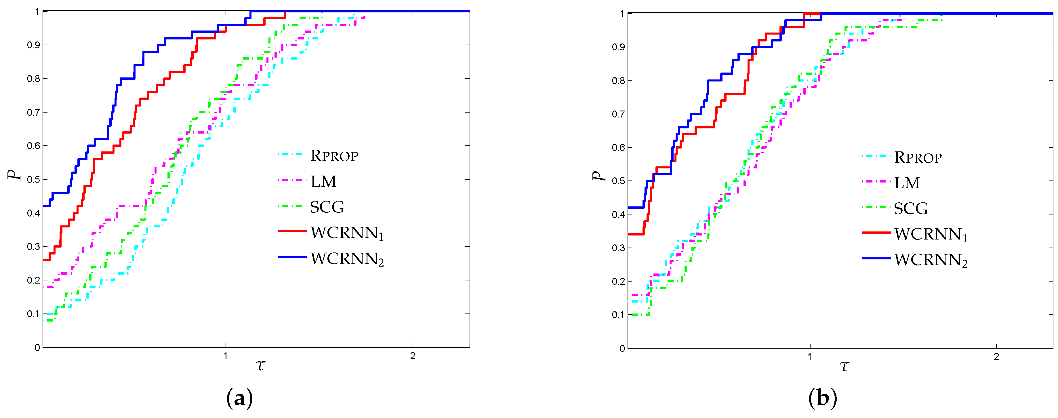
Furthermore, since a small number of simulations tends to dominate these results, the cumulative total for a performance metric over all simulations does not seem to be too informative. Therefore, similar to [13], we also utilized the performance profiles of Dolan and Morè [14] relative to both performance metrics, to present perhaps the most complete information in terms of robustness, efficiency, and solution quality. The use of performance profiles eliminates the influence of a small number of simulations on the benchmarking process and the sensitivity of results associated with the ranking of solvers. The performance profile plots the fraction P of simulations for which any given algorithm is within a factor $\tau$ of the best training algorithm. The curves in the following figures have the following meaning.

• “Rprop” stands for Resilient backpropagation.
• “LM” stands for Levenberg–Marquardt training algorithm.
• “SCG” stands for Scaled Conjugate Gradient.
• “WCRNN${}_1$” stands for Algorithm 1 with bounds $[-1,1]$ on all weights.
• “WCRNN${}_2$” stands for Algorithm 1 with bounds $[-2,2]$ on all weights.

4.1.1. Bank Marketing Dataset

The data were related to direct marketing campaigns (phone calls) of a Portuguese banking institution, and the classification goal was to predict if the client will subscribe to a term deposit. Each observation represented a customer and was described by 17 attributes, both categorical and continuous, corresponding to a total of 4119 contacts. During these phone campaigns, an attractive long-term deposit application, with good interest rates, was offered. For each contact, a large number of attributes was stored and if there was a success (the target variable). For the whole database considered, there were 451 successes (11% success rate) and 3668 failures (89% failure rate). The network architectures consisted of one hidden layer with 10 neurons and an output layer of two neurons, while the error goal was set to $E_G\le 0.05$ within the limit of 1000 epochs.

Figure 1 presents the performance profile for the bank marketing classification problem, investigating the performance of each training algorithm. Firstly, we note that both versions of the proposed training algorithm illustrated the highest probability of being the optimal training algorithm in terms of classification accuracy, since their curves lied on the top. More analytically, WCRNN${}_1$ and WCRNN${}_2$ reported 26% and 42% of simulations with the best $F_1$-score, respectively; while the state-of-the-art training algorithms Rprop, LM, and SCG presented 10%, 18%, and 6%, respectively. Furthermore, WCRNN${}_1$ and WCRNN${}_2$ reported 34% and 42% of simulations with the best accuracy, respectively; while the state-of-the-art training algorithms Rprop, LM, and SCG presented 14%, 16%, and 10%, respectively. Summarizing, we conclude that the application of the bounds on the weights of the RNNs increased the overall classification accuracy, in most cases. However, it is worth noticing that in case the bounds were too tight, this will not substantially benefit the classification performance.

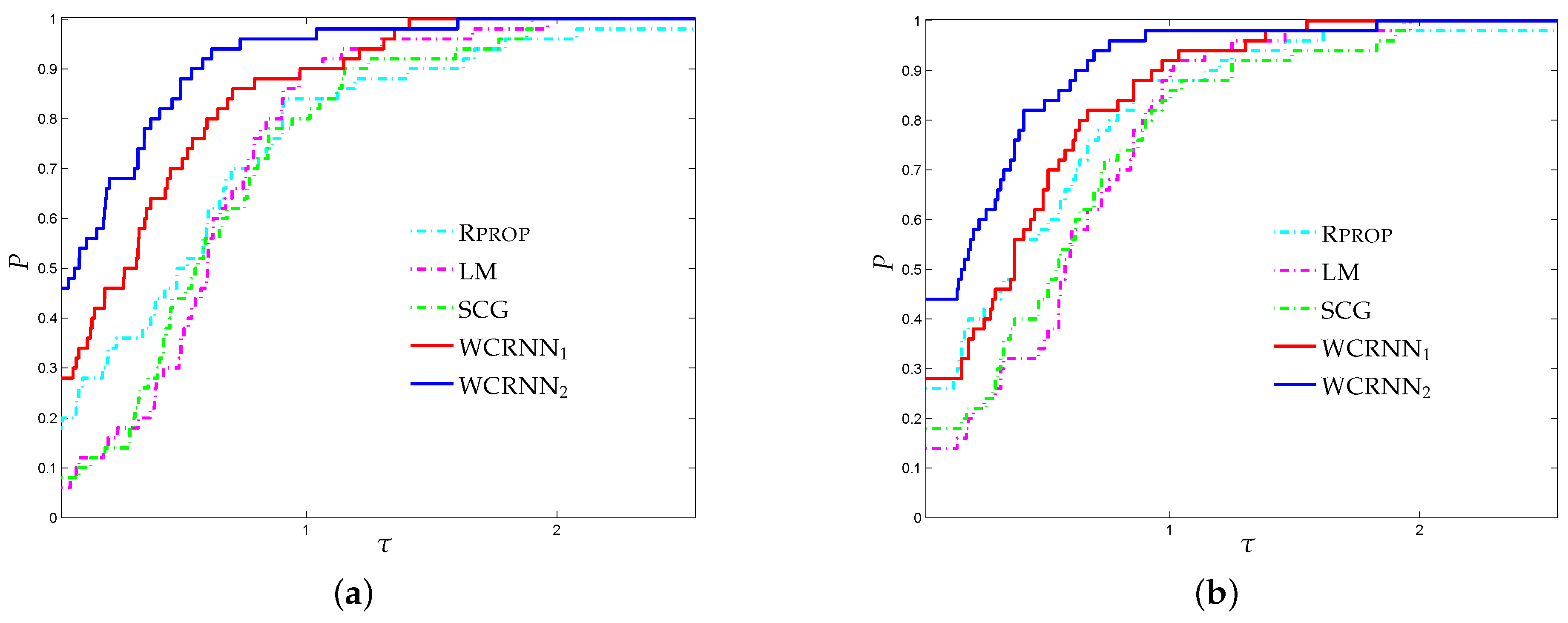
4.1.2. German Credit Approval Problem

The German credit approval dataset contained all the details concerning approved or rejected credit card applications in Germany. This imbalanced dataset was constituted by 1000 instances (300 negative decisions and 700 positive decisions), with 20 explanatory variables (seven continuous and 13 categorical) The interesting thing about this classification problem is that the data varied and had a mixture of attributes, which were continuous, nominal with small numbers of values, and nominal with larger numbers of values. The network architecture consisted of one hidden layer with 30 neurons and an output layer of two neurons, while the error goal was set to $E_G\le 0.1$ within the limit of 1000 epochs.

Figure 2a,b presents the performance profiles for the German credit approval classification problem, based on $F_1$-score and accuracy. Firstly, it is worth noting that WCRNN${}_1$ and WCRNN${}_2$ outperformed the classical training algorithms, presenting the highest probabilities of being the optimal solvers, relative to both performance metrics. Regarding the $F_1$-score metric, WCRNN${}_2$ exhibited the best performance, outperforming the rest of training algorithms, followed by WCRNN${}_1$. Furthermore, WCRNN${}_1$ and WCRNN${}_2$ reported 28% and 44% of simulations with the highest classification accuracy, respectively; while Rprop, LM, and SCG reported 26%, 14%, and 18%, respectively. Thus, the interpretation of Figure 2 demonstrates that the application of the bounds on the weights of the neural network increased the overall classification accuracy.

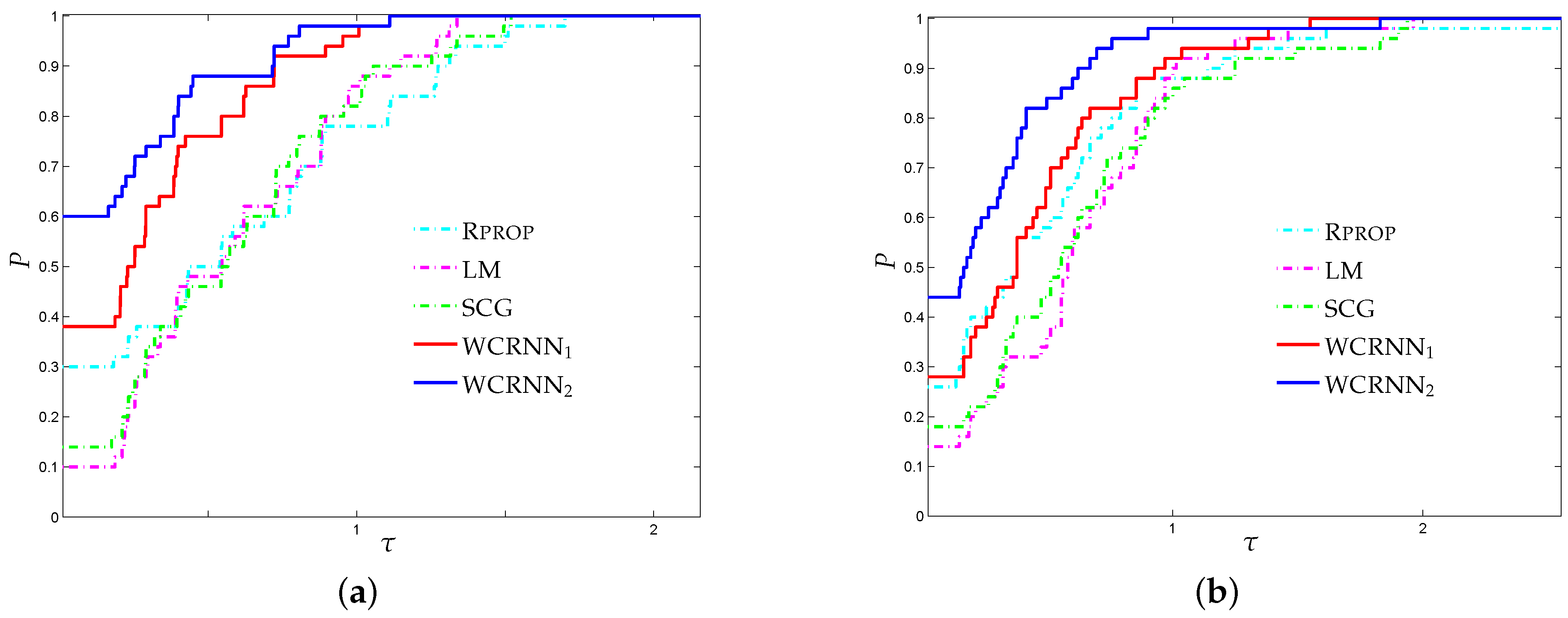
4.1.3. Banknote Authentication Problem

The data for this classification problem were extracted from images taken from genuine and forged banknote-like specimens. For digitization, an industrial camera usually used for print inspection was used. The final images had $400\times 400$ pixels. Due to the object lens and distance to the investigated object, gray-scale pictures with a resolution of about 660 dpi were gained. The wavelet transform tool was used to extract features from images. The network architectures consisted of 2 hidden layers with 8 and 4 neurons each and an output layer of 2 neurons, while the error goal was set to $E_G\le 0.01$ within the limit of 2000 epochs.

Figure 3 illustrates the performance profiles regarding the banknote authentication classification problem. It is worth noticing that WCRNN${}_2$ exhibited the highest probability of being the optimal solver, significantly outperforming all other training algorithms, followed by WCRNN${}_1$. More specifically, WCRNN${}_1$ and WCRNN${}_2$ reported 30% and 54% of simulations with the highest $F_1$-score, respectively; while the state-of-the-art training algorithms Rprop, LM, and SCG presented 24%, 8%, and 12%, respectively. Furthermore, WCRNN${}_1$ and WCRNN${}_2$ reported 38% and 60% of simulations with the highest classification accuracy, respectively; while the state-of-the-art training algorithms Rprop, LM, and SCG presented 30%, 10%, and 14%, respectively. Summarizing, we conclude that the application of the bounds on the weights of the RNNs increased the overall classification accuracy; however, in case the bounds are too tight, this will not substantially benefit the classification performance.

4.2. Performance Evaluation against State-of-the-Art Supervised Algorithms

In the sequel, we will evaluate the performance of the RNNs, which were trained with WCRNN algorithm against the state-of-the-art supervised algorithms, naive Bayes [25], Support Vector Machines (SVM) [26], 3NN [27], and random forest [28]. These classification models constitute some of the most effective and widely-used data mining algorithms for classification [29].

Table 1. Performance comparison of WCRNN${}_1$ and WCRNN${}_2$ against state-of-the-art classification algorithms, regarding $F_1$-score and accuracy.

Algorithm	${\mathit{F}}_1$-Score			Accuracy
	Bank	German	Banknote	Bank	German	Banknote
RNN (WCRNN${}_1$)	0.93	0.77	0.98	91.64%	74.73%	97.88%
RNN (WCRNN${}_2$)	0.93	0.77	0.98	91.70%	75.60%	98.11%
Naive Bayes	0.88	0.72	0.79	86.76%	72.80%	79.66%
SVM	0.88	0.71	0.92	90.02%	73.60%	92.41%
3NN	0.87	0.71	0.97	88.88%	72.40%	97.44%
Random Forest	0.91	0.74	0.98	91.30%	75.10%	98.32%

presents the performance comparison of WCRNN${}_1$ and WCRNN${}_2$ against state-of-the-art classification algorithms, relative to $F_1$-score and accuracy. Notice that the best performance is highlighted in bold for each metric. Random forest exhibited the best performance among state-of-the art classifiers, which is probably due to the fact that random forest is the only classifier based on an ensemble methodology. Nevertheless, the RNNs trained with WCRNN${}_1$ and WCRNN${}_2$ exhibited the highest average $F_1$-score, relative to all problems. Regarding the classification accuracy, the RNNs (WCRNN${}_2$) exhibited the best performance for bank marketing and German credit approval datasets, followed by RNN (WCRNN${}_1$). Moreover, random forest reported the highest accuracy for banknote authentication dataset, slightly outperforming the RNN (WCRNN${}_2$).

Summarizing, it is worth mentioning that the RNNs trained with both versions of WCRNN outperformed all state-of-the-art classifiers in terms of $F_1$-score. Furthermore, their classification performance was superior to all single classifiers and competitive with the ensemble-based random forest, regarding all benchmarks.

5. Conclusions

In this work, we evaluated the classification accuracy of weight-constrained recurrent neural networks in forecasting economic data. The classification efficiency of these new prediction models was based on a recently-proposed training algorithm, which exploits the numerical efficiency and very low memory requirements of the limited memory BFGS matrices, together with a gradient-projection strategy for handling the bounds on the weights. By placing constraints on the values of weights, the likelihood that some weights will “blow up” to unrealistic values is considerably reduced. Our numerical experiments demonstrated the classification efficiency of the proposed models, as confirmed statistically by the performance profiles. Therefore, we are able to conclude that the proposed algorithm appears to train RNNs efficiently with improved classification ability in domains such as forecasting economic benchmarks.

The determination of optimal bounds on the weights is a rather challenging task; therefore, more research and experiments are needed. To this end, the question of what should be the values of the bounds for each benchmark or what constraints should be applied to the weights of each layer is still under consideration. An interesting idea could be to auto-adjust the bounds during the training process utilizing a strategy based on the use of a validation set. Probably, the required research to answer these questions, may reveal additional and crucial information and questions.

Our future work is concentrated on incorporating the proposed methodology with more advanced and complex architectures such as long short-term memory neural networks and deep neural networks, together with sophisticated techniques such as dropout and batch normalization. Since our experimental results are quite encouraging, a next step could be the evaluation of the proposed framework for the prediction of stock exchange index movement and for forecasting the value of stock price indices and prices. Furthermore, another interesting aspect for future research could be the utilization of rule induction and discovery methods or even the use of synthetic data for further accuracy improvement based on the insights received in their training/testing periods (see [30,31] and the references therein). Finally, we intend to conduct extensive empirical experiments by applying the proposed algorithm in specific scientific fields and to evaluate its performance on large real-world datasets, such as educational, healthcare, etc.