A Novel Coupling Algorithm Based on Glowworm Swarm Optimization and Bacterial Foraging Algorithm for Solving Multi-Objective Optimization Problems

Abstract

In the real word, optimization problems in multi-objective optimization (MOP) and dynamic optimization can be seen everywhere. During the last decade, among various swarm intelligence algorithms for multi-objective optimization problems, glowworm swarm optimization (GSO) and bacterial foraging algorithm (BFO) have attracted increasing attention from scholars. Although many scholars have proposed improvement strategies for GSO and BFO to keep a good balance between convergence and diversity, there are still many problems to be solved carefully. In this paper, a new coupling algorithm based on GSO and BFO (MGSOBFO) is proposed for solving dynamic multi-objective optimization problems (dMOP). MGSOBFO is proposed to achieve a good balance between exploration and exploitation by dividing into two parts. Part I is in charge of exploitation by GSO and Part II is in charge of exploration by BFO. At the same time, the simulation binary crossover (SBX) and polynomial mutation are introduced into the MGSOBFO to enhance the convergence and diversity ability of the algorithm. In order to show the excellent performance of the algorithm, we experimentally compare MGSOBFO with three algorithms on the benchmark function. The results suggests that such a coupling algorithm has good performance and outperforms other algorithms which deal with dMOP.

1. Introduction

With the development of society, more and more real optimization problems involving industrial and scientific problems are common [1,2,3]. Usually, these optimization problems are noy independent, but rather a set of objective functions. The optimization problems with a set of objective functions are known as multi-objective optimization (MOP). In general, MOP requires a set of optimal tradeoff solutions in the case of two or more conflicting objectives. Typical examples include scheduling problems with available resources, vehicle routing in traffic networks of traffic flow, etc.

Generally speaking, Swarm intelligence optimization algorithms (SIOAs) are mostly inspired by the behaviors of biological swarm systems (e.g., bird flocking, foraging and courtship).There are several popular SIOAs, such as genetic algorithm (GA) [4], differential evolution algorithm (DE) [5], particle swarm optimization (PSO) [6,7], ant colony optimization (ACO) [8], artificial bee colony (ABC) [9,10], bat algorithm (BA) [11,12], bacteria foraging optimization algorithm (BFOA) [13], cuckoo search (CS) [14,15,16] and glowworm swarm optimization (GSO) [17,18], etc. In the past decades, these SIOAs have been widely applied to various optimization problems [19,20]. When projects or systems in real-life become large, some very complex optimization problems emerge, such as large-scale optimization problems and multi-objective optimization problems (MOPs). However, for these problems, it is found that these algorithms are originally designed to solve simple practical problems and the algorithms will not be suitable for solving the complex practical problems. So, the performance of most SIOAs encounters great challenges. Therefore, strong and effective SIOAs are required.

Up to now, most Swarm intelligence optimization algorithms have been proposed to solve multi-objective optimization problems. For example, Deb et al. proposed NSGA [21]. The algorithm is implemented hierarchically according to the dominance and non-dominance relations between individuals. However, the algorithm’s performance is affected by the high computational complexity of this algorithm, non-elitism strategy and relies heavily on Shared parameters. In 2000, Deb suggests a non-dominated sorting based on muli-objective evolutionary algorithms (MOEAs), called non-dominated sorting genetic algorithm II (NSGA-II) [22] to address these issues. Zhang et al. proposed MOEA/D [23], which is to decompose MOPs into multiple scalar sub-problems, and then the sub-problems are simultaneously optimized. Horn et al. proposed NPGA [24], which integrated the concept of Pareto dominance into the selection operation of GA and applied the niche to the entire population. Zitzler et al. proposed SPEA2 [25], which tried to mix adaptive value allocation, archive truncation, and the density selection strategies. Gong et al. [26] use of the strength Pareto genetic algorithm (GA) with immunity as a tool to solve multi-objective optimization problems in the maintenance of aircraft equipment and propose the PNIA algorithm.

In this paper, we focus on improving SIOAs for solving MOPs. As can be seen from the above review, most swarm intelligence algorithms have their own advantages and disadvantages. According to the no free lunch theorem [27], it is difficult to use one algorithm to solve all kinds of optimization problem. Recently, an ensemble strategy was proposed to benefit from both the availability of diverse approaches and the need to tune the associated parameters. The research has shown the general applicability of the ensemble strategy in solving diverse problems by using different populated optimization algorithms [28]. What’s more, the coupling rules are different such as the parallel method, serially method, and nested method, and so on. At present, there are many coupling algorithms in the research and the method has become a new research hotspot. Therefore, a new idea is formed by coupling two or more strategies of algorithms to make the algorithm inherit the advantages of different algorithms and overcome the disadvantages of a single algorithm. In this paper, a coupling algorithm is designed for many-objective optimization based on GSO and BFO to deal with the MOPs [29,30]. As we all know, a good balance between exploration and exploitation is important for optimization algorithm. MGSOBFO is proposed to achieve a good balance between exploration and exploitation by dividing into two parts. Part I is in charge of exploitation by GSO and the Part II is in charge of exploration by BFO. At the same time, the simulation binary crossover (SBX) [22] and polynomial mutation [22] are introduced into the MGSOBFO to enhance the convergence and diversity ability of the algorithm. Those methods not only have an effect on the convergence ability of the algorithm, but also have the effect of extending the coverage of population to avoid being trapped into the local optimum.

The rest of the article is organized as follows. In Section 2, we give a brief introduction of multi-objective optimization problems and standard GSO, BFO algorithm. In Section 3, we introduce the detail of proposed approach. Section 4 gives out the comparison results and experimental analyses of MGSOBFO algorithm. Finally, Section 5 gives some conclusions of the work and directions for future work.

2. Basic Concepts

2.1. The Multi-Objective Optimization Problems

In general, a multi-objective optimization problem can be defined as a vector function f that maps a tuple of n decision variables to tuple of m objectives.

Formally as follow:

$$\begin{gathered} Min y=f(x)=(f_1(x),f_2(x),\cdots ,f_m(x)) \\ subject to x=(x_1,x_2,\cdots x_n)\in R^n \end{gathered}$$

(1)

where $x$ is called the decision vector, and $f_m(x)$ is the m-th sub-objective function. $R^n$ is parameter (decision variables) space.

As we all know that the objectives in multi-objective optimization problems are conflicting, no single solution can be found to be best in all solutions. So, the best tradeoffs among the objectives can be defined in terms of Pareto optimality. A solution vector $x^a={(x_1^a,x_2^a,\cdots ,x_n^a)}^T$ is said to dominate another vector $x^b={(x_1^b,x_2^b,\cdots ,x_n^b)}^T$ if and only if $x_i^a\le x_i^b$ for $\forall i\in \{1,2,\cdots ,n\}$ and $\exists i\in \{1,2,\cdots ,n\}$. The dominance relationship can be described like this: $x_i^a\prec x_i^b$ [31].

2.2. Standard Glowworm Swarm Optimization Algorithm (GSO)

Glowworm Swarm Optimization (GSO) [17,18] is a novel swarm intelligence search algorithm. The idea of the algorithm is to simulate the social behaviors of fireflies in nature by using fluorescein to make connections. The standard GSO algorithm consists of four stages, namely, the initialization, the updating luciferin, the updating position and the updating perception range stage. The following four stages of operation are described in detail.

(1)

Initialization

In the initialization stage, fireflies are randomly distributed in the decision feasible region. In addition, the initial luciferin and the sensing radius is the same for each firefly.

(2)

Updating luciferin

The luciferin of firefly is directly related to its location in the search space. And the higher the evaluation value of the position in the space, the higher the fitness of the individual, that is, the larger the fluorescent of the individual. The specific equation of updating fluoresce in is as follows.

$$l_i(t+1)=(1-\rho )l_i(t)+\gamma J(x_i(t+1))$$

(2)

where $\rho$ denotes the luciferin volatility parameters of firefly; $l_i(t)$ denotes the luciferin value of the firefly $i$ in the $t\mathrm{th}$ iteration; $\gamma$ denotes the updating luciferin rate parameters of firefly; $J(x_i(t+1))$ denotes the evaluation value of firefly $i$ at position $x_i(t+1)$ in the t+1th iteration.

(3)

Roulette selection

For each iteration, the fireflies need to find the firefly that the luciferin value is larger than its own within the sensing range of the firefly. Then, the updating direction of the firefly position should be determined according to the roulette method. In addition, the selection probability of the neighboring firefly is also determined according to the luciferin value. The GSO algorithm will selects the individuals that meet the following two conditions to form a group.

• Glowworm $j$ needs to be within the perceived radius of glowworm $i$;
• The luciferin of glowworm $j$ is brighter than that of glowworm $i$.

The specific equation for the selection probability of the neighboring firefly is as follows.

$$p_{ij}(t)=\frac{l_j(t)-l_i(t)}{{\displaystyle \sum _{k\in N_i(t)}{l}_k(t)-l_i(t)}}$$

(3)

$$N_i(t)=\{j:d_{i,j}(t)<r_d^i;l_i(t)<l_j(t)\}$$

(4)

where, $j\in N_i(t)$, and $N_i(t)$ represents the neighborhood set of firefly i in the tth iteration; $r_d^i(t)$ represents the decision radius of firefly i in the tth iteration; $d_{i,j}(t)$ represents the space distance between firefly i and j in the tth iteration; $p_{ij}(t)$ represent sthe probability of firefly i to firefly j in the tth iteration.

When the neighborhood firefly j of firefly i is selected, firefly i will update its position as the following update equation.

$$x_i(t+1)=x_i(t)+s\ast (\frac{x_j(t)-x_i(t)}{\Vert x_j(t)-x_i(t)\Vert })$$

(5)

where, s represents the moving step size of firefly; $\Vert x_j(t)-x_i(t)\Vert$ represents the Euclidean space distance between firefly i and firefly j.

(4)

Neighborhood range update rule

After the position of the firefly is updated, the range of perception will be dynamically adjusted. The size of the perceived radius is determined by the number of firefly individuals within the perceived radius. The specific equation of the updating perceptual range is as follows.

$$r_d^i(t+1)=\min \{r_s,\max \{0,r_d^i(t)+\beta \ast (n_t-\left|N_i(t)\right|)\left\}\right\}$$

(6)

where, $r_s$ represents the perception radius; $n_t$ represents the threshold for firefly neighborhood set; $\beta$ is the parameter to adjust the size of firefly’s dynamic perception range.

2.3. Standard Bacterial Foraging Algorithm (BFO)

Passino proposed an algorithm BFO [13] to solve corresponding problems in 2001.Compared with the well-known EAs DE, genetic algorithm, and PSO, BFO shows excellent performance. The bacterial foraging optimization algorithm is inspired by the foraging strategies of the E. Coli bacterium cells. The basic principle of the bacterial foraging algorithm is to regard each Escherichia coli as a solution. BFO complete the search process of the optimal solution by the bacterial foraging behavior: chemotaxis, swarming, reproduction and elimination. The four parts are as follows:

➢

The Chemotaxis

Chemotaxis is achieved by the following two operations: swimming and tumbling. When a bacterium meets a favorable environment, it will continue swimming in the same direction. When it meets an unfavorable environment, it will tumble. The process of movement can be defined as follow:

$$x^i(j+1,k,l)=x^i(j,k,l)+C(i)\frac{\Delta (i)}{\sqrt{{\Delta }^{\mathsf{{\rm T}}}(i)\bullet \Delta (i)}}$$

(7)

where $x^i(j,k,l)$ represents the position of bacteria $i$ when it approaches the $j\mathrm{th}$ reproduction and $l\mathrm{th}$ elimination and dispersal; $C(i)$ is the step of chemotaxis; $\frac{\Delta (i)}{\sqrt{{\Delta }^{\mathsf{{\rm T}}}(i)\bullet \Delta (i)}}$ is a random forward direction of movement.

Assuming that the objective function value of bacteria $i$ at $x^i(j+1,k,l)$ is $f(x^i(j+1,k,l))$, bacteria $i$ will continue to move in the same direction until the value of the objective function no longer decreases or the maximum number of steps is reached when $f(x^i(j+1,k,l))<f(x^i(j,k,l))$. In a sense, chemotaxis operation is a complex movement process interwoven with the operation of tumble and swimming, in which tumble represents the direction of optimization and swimming represents the degree of searching feasible solutions in a certain direction.

➢

The Swarming

In the BFO algorithm, each of individual does not independently. They release two signals in the process of foraging, one called the attractor signal, the other called the rejection signal. The attractive signal is mainly used to attract other bacteria to get close to itself, while the repulsive signal is used to limit the distance between other bacteria individuals and themselves. So, the swarming can be expressed by (8), (9):

$$\begin{array}{ll}{f}_{cc}(x^i,P(j,k,l))& ={\displaystyle \sum _{r=1}^S{f}_{cc}(x^i,x^r(j,k,l))}\\ & ={\displaystyle \sum _{r=1}^S[-d_{attract\mathrm{an}t}\exp {(-w_{attrac\tan t}{\displaystyle \sum _{p=1}^n(x_p^i-x_p^r})}^2)]}\\ & +{\displaystyle \sum _{r=1}^S[h_{repellent}\exp {(-w_{repellent}{\displaystyle \sum _{p=1}^n(x_p^i-x_p^r})}^2)]}\end{array}$$

(8)

$$J(i,j+1,k,l)=J(i,j,k,l)+f_{cc}$$

(9)

where $f_{cc}(x^i,P(j,k,l))$ represent a objective function that varies with the population distribution. $d_{attract\mathrm{an}t}$ and $w_{attract\mathrm{an}t}$ represent the release quantity and diffusion rate of inducement signal, respectively, and $h_{repellent}$ and $w_{repellent}$ represent the release quantity and diffusion rate of rejection signal, respectively.

➢

The Reproduction

With the continuous absorption of nutrients, E. coli will gradually grow as nutrients continue to be absorbed. Under appropriate conditions, each E. coli will asexually split into two bacteria. However, the bacteria will be eliminated for those bacteria with poor nutrition. In the reproduction, $J_{health}^i$ is used to represent the energy value of the ith bacteria, which determines the foraging ability of bacteria. And then the bacteria are sorted according to their health values. The bacteria with healthy values ranked in the first half are used for reproduction and the other half of bacteria are eliminated. The new reproduction has exactly the same foraging ability as the original bacteria. The value of $J_{health}^i$ is calculated by:

$$J_{health}^i={\displaystyle \sum _{j=1}^{N_c}f(x^i(j,k,l))}$$

(10)

where $J_{health}^i$ represents the energy value of the ith bacteria; $N_c$ indicates the number of chemotaxis; $f(x^i(j,k,l))$ is the fitness value of the ith bacteria after the jth chemotaxis, the kth reproduction and the lth elimination and dispersal operations.

➢

The Elimination and Dispersal Operation

After the reproduction, the bacteria will execute the elimination and dispersal operation with a certain probability. The basic principle of elimination and dispersal operation is similar to the mutation operation in genetic algorithm, which can continue to search in unexploited areas and prevent the population from falling into local minima. The migration operation can be defined as follow:

$$x=\{\begin{array}{ll}{x}_{new},& if q<p_{ed}\\ x,& otherwise\end{array}$$

(11)

where $x_{new}$ denotes the new position obtained through initialization, $q,(0<q<1)$ is a uniformly distributed random number.

3. The MGSOBFO Algorithm

At the beginning, the GSO and BFO algorithm was proposed to solve the single objective optimization problem rather than multi-objective optimization problems (MOPs). Therefore, it is meaningful to improve the corresponding strategies so that these two algorithms can be used to solve multi-objective optimization problems. In this paper, we proposed a new coupling algorithm based on GSO and BFO (MGSOBFO). Next, we will introduce each process from a single target algorithm to multi-target algorithm.

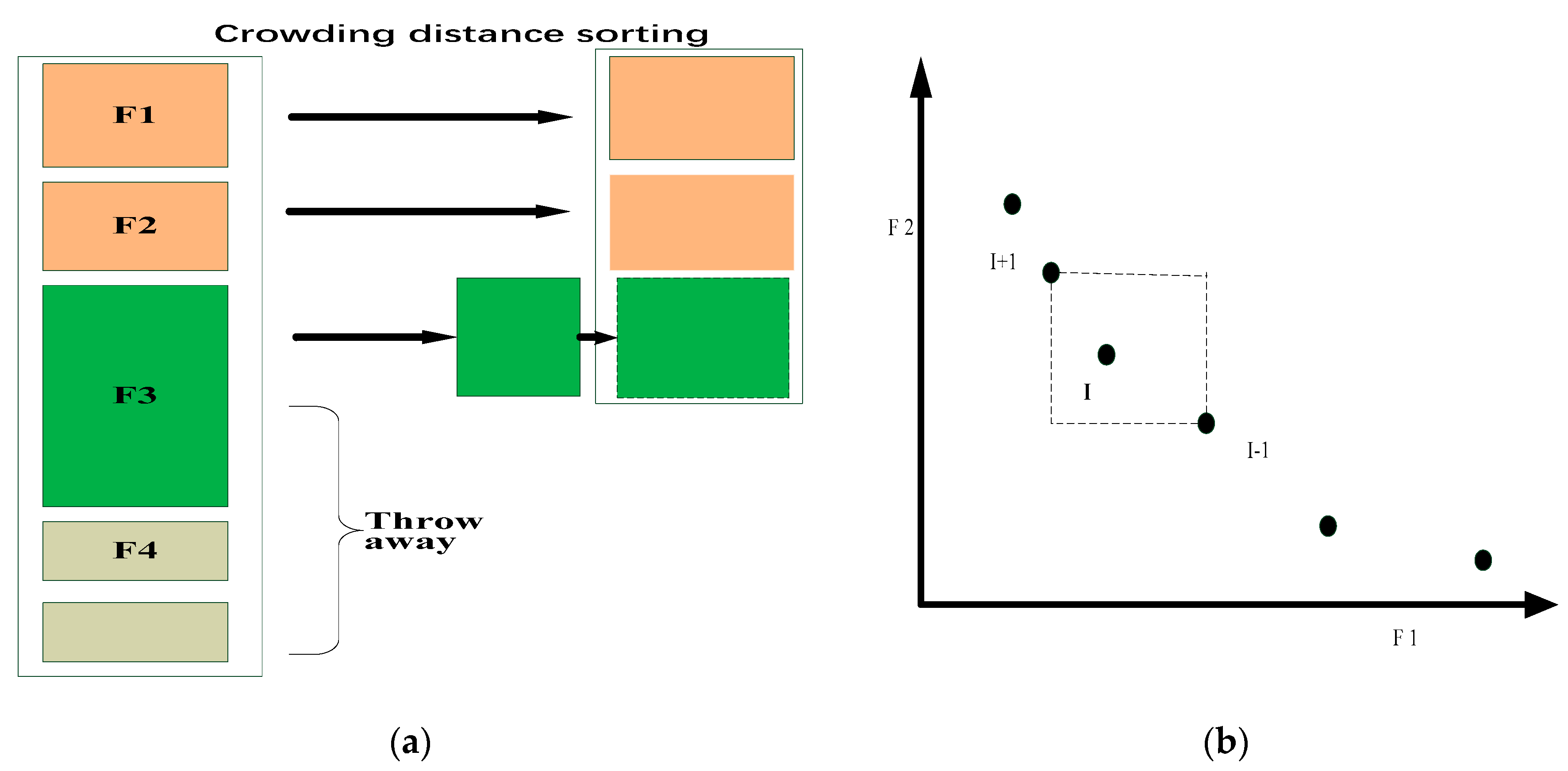
3.1. Fast Non-Dominated Sorting Approach and Crowding Distance

Before introducing the multi-objection firefly bacteria foraging algorithm, we first introduce the following two basic concepts: fast non-dominant sorting and crowding distance [22].

(1)

Fast Non-dominated Sorting Approach

First, we calculated two values for each solution.① domination count $N_p$, the number of solutions which dominate the solution q. ② $S_q$, a set of solutions that the solution q dominates. The pseudo code of the MaBFOA operator is listed in Algorithm 1:

Algorithm 1: Fast non-dominated sort approach

for each $p\in P$ $S_p=0$, $n_p=0$  for each $q\in P$ if $p\prec q$       // if p dominated q then $S_p=S_p\cup \left\{q\right\}$

else if $q\prec p$ then $n_p=n_p+1$  end if $n_p=0$ then $p_{rank}=1$     // p belong to the first front

$F_1=F_1\cup \left\{p\right\}$

end

i = 1        //Initialize the front counter

While $F_1\ne 0$, $Q=0$//Q represents the next front for store

For each $q\in S_p$ $n_q=n_q-1$ if $n_q=0$//q belong to the next front then $q_{rank}=i+1$,

$Q=Q\cup \left\{q\right\}$ i=i+1 $F_i=Q$

end

(2)

Crowding-distance calculation approach

The crowding distance sorting procedure is shown in Figure 1a. The crowding-distance computation requires sorting the population according to each objective function value in ascending order of magnitude. All populations’ members are assigned a distance metric; we can compare two solutions for their extent of proximity with other solutions. The boundary solutions are assigned an infinite distance value. In Figure 1b, the crowding-distance of the I-th solution in its front is the side length of the cuboids. The crowded-comparison operator guides the selection process towards a uniformly spread-out Pareto-optimal front. The crowding distance of each individual be computed by Equation (12).

$$d_i={\displaystyle \sum _{k=1}^m\left|f_k(i-1)-f_k(i+1)\right|}$$

(12)

In most situations, the last level is accepted partially. In such a case, these solutions with better crowding distances are picked up.

3.2. The Self-Adaptive for Chemotaxis

As we all know, in the bacterial foraging algorithm of single objective, we know that the best individual is chosen when the bacterial move one. However, in the multi-objective algorithm, the advantages and disadvantages by comparison between individuals cannot be concluded by comparing only one adaptive value as in the single-objective algorithm. Therefore, here we define a new Pareto dominance relation to compare two individuals.

In the MGSO-BFO, assuming that $x_1$ and $x_2$ are any two individuals in the population. The dominant relationship between $x_1$ and $x_2$ is defined as follows:

(a)

if $x_i^{}\underset{-}{\prec }{x}_j^{}$, that means $x_i^{}$ is better than $x_j^{}$;

(b)

if $x_j^{}\underset{-}{\prec }{x}_i^{}$, that means $x_j^{}$ is better than $x_i^{}$;

(c)

If there is no dominant relationship between $x_i^{}$ and $x_j^{}$, normalization is carried out for different fitness values. The process is as follows:

Firstly, the proportion $w$ of the two individuals in the objective value is calculated, respectively.

$$W_i=\frac{f_i}{f_i+f_j}$$

(13)

$$W_j=\frac{f_j}{f_i+f_j}$$

(14)

Finally, the sum of weighted is given as follows:

$$F={\displaystyle \sum _{k=1}^M{\delta }_k\ast |W_j-W_i|}$$

(15)

where ${\delta }_k$ $(0<{\delta }_k<1,and{\displaystyle \sum _{k=1}^M{\delta }_k=1})$ represents the weight coefficient of each objective, $M$ represents the number of objective functions.

In the chemotaxis operation, each position of an individual is compared by above the Pareto dominance relationship mentioned. However, in the original algorithm, the original fixed step size cannot meet the requirements of convergence. So, there we make a new definition of the step size. The calculation formula is shown as follow:

$$C_D=\frac{S_D}{j+k+l}$$

(16)

where $C_D$ represents the initialization step size in the D dimension, $S_D$ represents the step size in the D dimension. $j,k,l$ represents the chemotaxis, replication and dispersion, respectively.

It can be seen from the above formulas that $C_D$ is large, which is conducive to global search at the beginning. With the iteration of the algorithm, it is conducive to local search in the later stage of the algorithm.

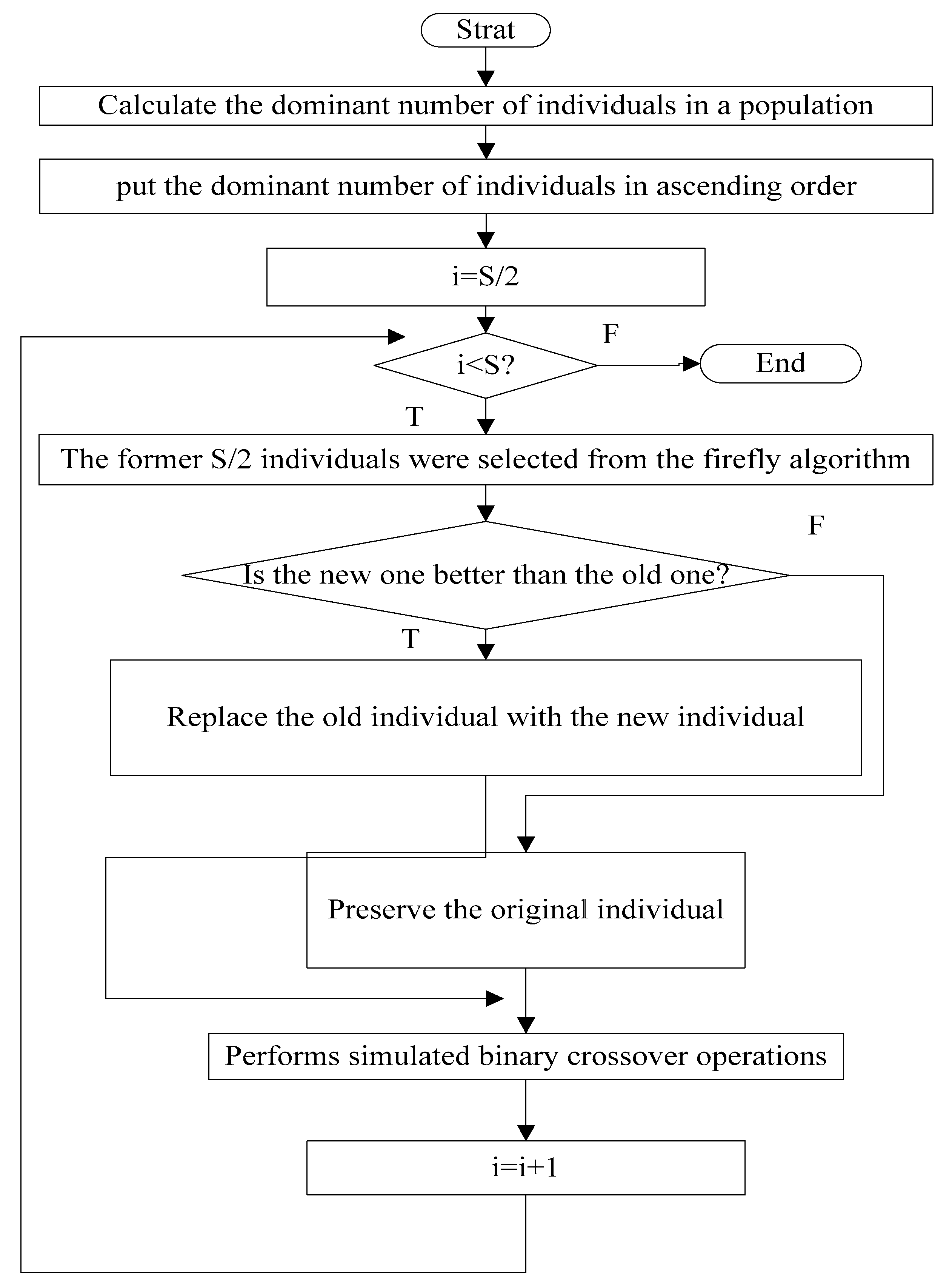
3.3. The Replication Operations Based on Crossover

In the standard BFO algorithm, the replication operation is to sort individuals according to the size of the function’s adaptive value, and then replace the poor half with the good half. However, in the case of multi-objective, this operation will lead to a great decrease in the diversity of the population, which is not conducive to the diversity distribution of the population. In this section, in order to maintain the diversity of the population, we introduce the better individuals in GSO into it, and perform crossover operations between the two. The simulated binary crossover is shown below:

$$X_{1j}^{\prime }(t)=0.5\ast [(1+{\gamma }_j)\ast X_{1j}(t)+(1-{\gamma }_j)\ast X_{2j}(t)]$$

(17)

$$X_{2j}^{\prime }(t)=0.5\ast [(1-{\gamma }_j)\ast X_{1j}(t)+(1+{\gamma }_j)\ast X_{2j}(t)]$$

(18)

where ${\gamma }_j=\{\begin{array}{l}{(2u_j)}^{\frac{1}{\eta +1}}\hspace{1em}\hspace{1em}\mathrm{if} u_j\le 0.5\\ {(\frac{1}{2(1-u_j)})}^{\frac{1}{\eta +1}}\hspace{1em}\hspace{1em}other\end{array}$, $u_j\in \mathrm{U}(0,1)$, $\eta =1$.

The improved for replication operation as shown in Figure 2.

3.4. The Elimination and Dispersal Operations Based on Mutation

Generally speaking, we only consider the speed and accuracy of convergence in the single-objective optimization algorithm, but in the multi-objective optimization algorithm, we not only consider the convergence of the algorithm but also the diversity of the population. In the elimination and dispersal, they are randomly generated again for the individuals that meet certain conditions. Although this method can improve the diversity of the population to a certain extent, it does not make use of the convergence of the later algorithm in multi-objective optimization. In order to improve the convergence of the algorithm, polynomial mutation is introduced in the paper. The process of polynomial mutation is shown as fellow:

$${\mathrm{X}}_{1\mathrm{j}}^{\prime }(t)={\mathrm{X}}_{1\mathrm{j}}(t)+{\beta }_{\mathrm{j}}$$

(19)

where ${\beta }_{\mathrm{j}}=\{\begin{array}{l}{(2u_j)}^{\frac{1}{\eta +1}}-1\hspace{1em}\hspace{1em}{u}_j<0.5\\ (1-{(2(1-u_j))}^{\frac{1}{\eta +1}}other\end{array}$, $u_j\in \mathrm{U}(0,1)$, $\eta$ is the distribution exponent.

Through the above dispersing operation, the entire algorithm no longer disperses individuals randomly as before, but disperses individuals on a certain basis, which will be conducive to searching for better solutions.

3.5. The Flow Chart of MGSO-BFO

The flow chart of MGSO-BFO as show in Algorithm 2.

Algorithm 2: The MGSO-BFO

Step 1: Create a random population N of size S, and initialize the required parameters;    Step 2: Randomly generate the initial population    Step 3: Elimination and Dispersal Operations loop: let j=0, j = j + 1, $N_{ed}$ (the number of Elimination and Dispersal Operations step);    Step 4: The replication operations loop: let k = 0, k = k + 1; $N_{re}$ (the number of replication step)    Step 5: Chemotactic loop: let L = 0, L = L + 1; $N_c$ (the number of chemotactic step)    Take the chemotactic step for the ith bacterium as follows:      I. Calculate fitness function ${\theta }_i$ for all objective functions.      II. let $J={\theta }_i$, (save a better fitness may be found so far)      III. Tumble: create a random vector $\frac{\Delta (i)}{\sqrt{{\Delta }^{\mathsf{{\rm T}}}(i)\bullet \Delta (i)}}$      IV. Make movement with a self-adaption step(Specific see Formula (16)) for ith bacterium in direction. $\hspace{1em}\hspace{1em}\hspace{1em}\hspace{1em}\hspace{1em}\hspace{1em}\hspace{1em}\hspace{1em}\hspace{1em}\hspace{1em}\hspace{1em}\hspace{1em}\hspace{1em}{\theta }^i(j+1,k,l)={\theta }^i(j,k,l)+C(i)\frac{\Delta (i)}{\sqrt{{\Delta }^{\mathsf{{\rm T}}}(i)\bullet \Delta (i)}}$      V. Computer ${\theta }_i$ for all objective functions.      VI. Swim:       Let m = 0 (m respect the swim length counter)      While $m<N_s$        (1) Let m = m + 1        (2) If ${\theta }_i\prec J$ (${\theta }_i$ dominated $J$), let $J={\theta }_i$        (3) ues ${\theta }^i(j+1,k,l)={\theta }^i(j+1,k,l)+C(i)\frac{\Delta (i)}{\sqrt{{\Delta }^{\mathsf{{\rm T}}}(i)\bullet \Delta (i)}}$ to computer the new ${\theta }_i$.      VII. If $i\le S$, go to process the next bacterium.    Step 6: if $L<N_c$, go to the Step5    Step 7: The replication operations:    I. Perform non-dominated sorting of BFO and GSO, and identify different front $F_1,F_2,\cdots$    II. Prepare composite population by combining the BFO (s/2) with GSO (s/2).    III. Performs simulated binary crossover operations    IV. Select a new population of size S from the composite population.    IV. if $k<N_{re}$, go to the Step4    Step 8: Elimination and Dispersal Operations    I. For each bacterium $i$, if $rand<{\rho }_{ed}$, use the mutation process shown in Section 3.4.    II. if $j<N_{ed}$, go to the Step 3, else go to Step 9.    Step 9: End.

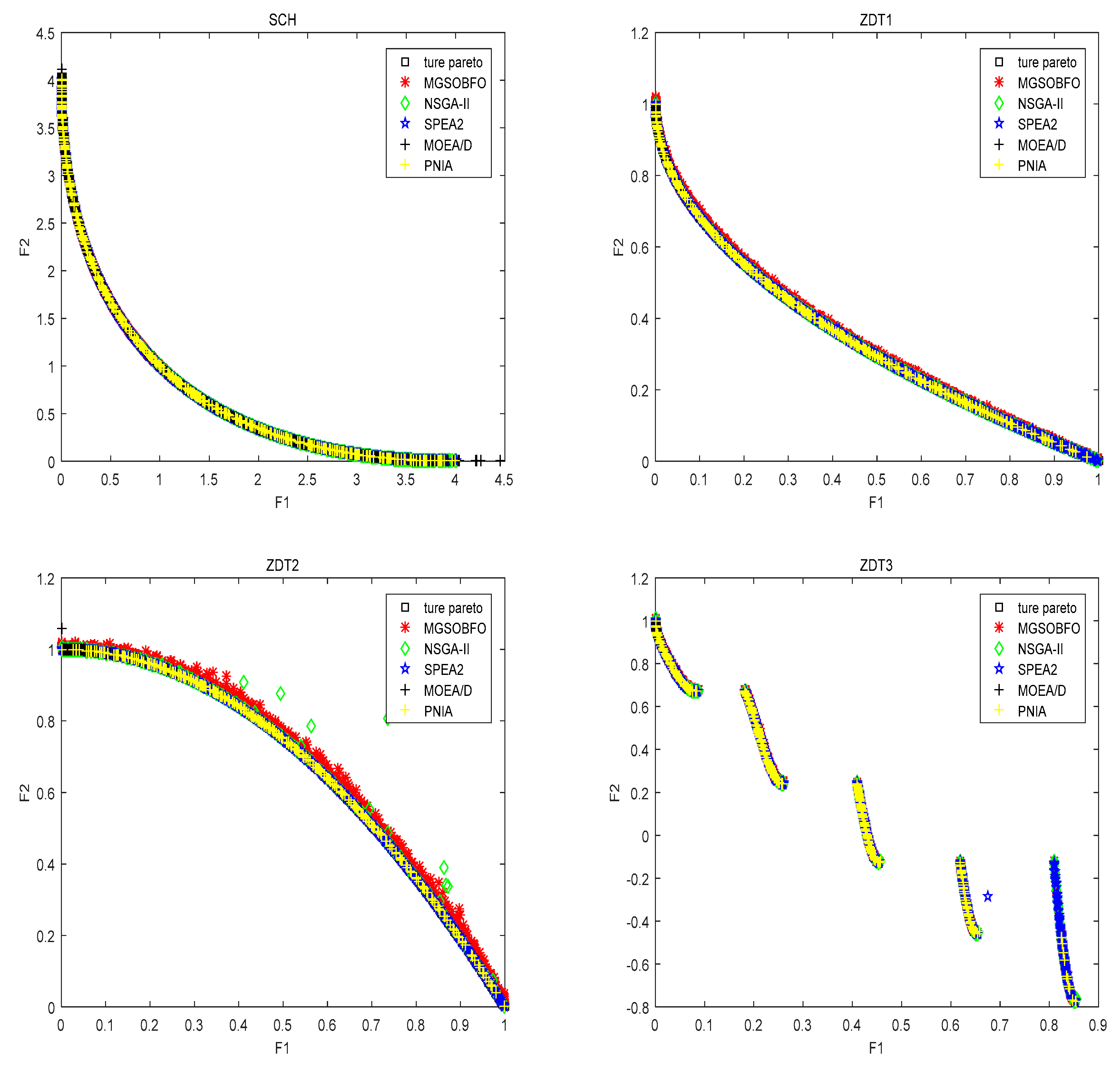
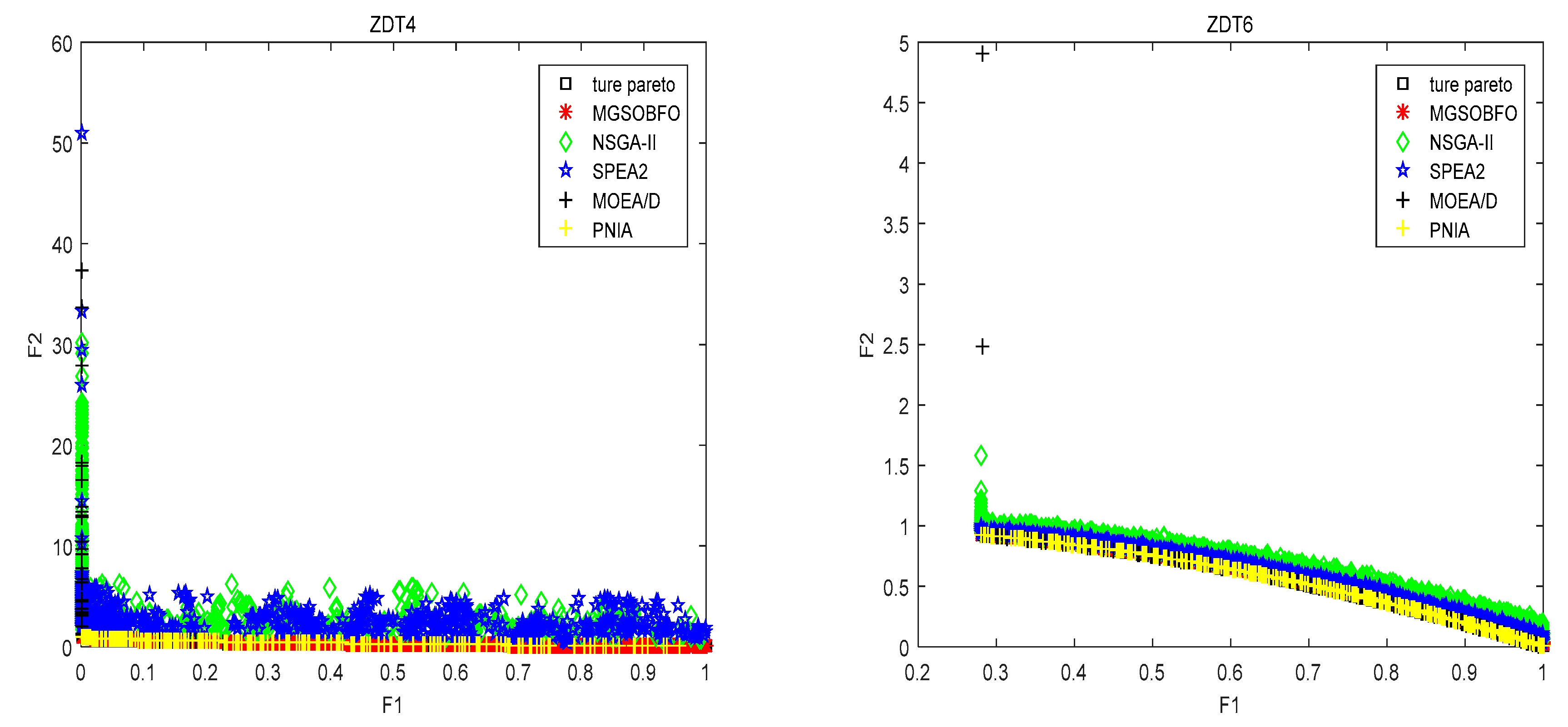
4. Experimental and Discussion

4.1. Test Set and Performance Measures

In the experiment, we use two benchmark sets ZDT [32] and SCH [33] test the performance of MGSO-BFO. For the ZDT test sets, it consists of six test instances, and we use five of them in the experiment. For more details about the test problems, please refer to

Table 1. six test function for multi-objective optimization algorithm.

Function	Dimension	Range	Objective Function	Optimal Solution	Feature
SCH	1	$[-{10}^3,{10}^3]$	$\begin{array}{l}{f}_1(x)=x^2\\ f_2(x)={(x-2)}^2\end{array}$	$x\in [0,2]$	convex
ZDT1	30	[0, 1]	$\begin{array}{l}{f}_1(x)=x_1\\ f_2(x)=g(x)[1-\sqrt{\frac{x_1}{g(x)}}]\\ g(x)=1+9\frac{{\displaystyle \sum _{i=2}^n{x}_i}}{n-1}\end{array}$	$\begin{array}{l}{x}_1\in [0,1]\\ x_i=0\\ i=2\cdots n\end{array}$	convex
ZDT2	30	[0, 1]	$\begin{array}{l}{f}_1(x)=x_1\\ f_2(x)=g(x)[1-{(\frac{x_1}{g(x)})}^2]\\ g(x)=1+9\frac{{\displaystyle \sum _{i=2}^n{x}_i}}{n-1}\end{array}$	$\begin{array}{l}{x}_1\in [0,1]\\ x_i=0\\ i=2\cdots n\end{array}$	Non-convex
ZDT3	30	[0, 1]	$\begin{array}{l}{f}_1(x)=x_1\\ f_2(x)=g(x)[1-\sqrt{\frac{x_1}{g(x)}}-\frac{x_1}{g(x)}\sin (10\pi x_1]\\ g(x)=1+9\frac{{\displaystyle \sum _{i=2}^n{x}_i}}{n-1}\end{array}$	$\begin{array}{l}{x}_1\in [0,1]\\ x_i=0\\ i=2\cdots n\end{array}$	convex discon-nected
ZDT4	10	$\begin{array}{l}{x}_1\in [0,1]\\ x_i\in [-5,5]\\ i=2\cdots n\end{array}$	$\begin{array}{l}{f}_1(x)=x_1\\ f_2(x)=g(x)[1-\sqrt{\frac{x_1}{g(x)}}]\\ g(x)=1+10(n-1)+{\displaystyle \sum _{i=2}^n[x_i^2}-10\cos (4\pi x_i)]\end{array}$	$\begin{array}{l}{x}_1\in [0,1]\\ x_i=0\\ i=2\cdots n\end{array}$	Non-convex
ZDT6	10	[0, 1]	$\begin{array}{l}{f}_1(x)=1-\exp (-4x_1){\sin }^6(6\pi x_1)\\ f_2(x)=g(x)[1-{(\frac{f_1(x)}{g(x)})}^2]\\ g(x)=1+9{(\frac{{\displaystyle \sum _{i=2}^n{x}_i}}{n-1})}^{0.25}\end{array}$	$\begin{array}{l}{x}_1\in [0,1]\\ x_i=0\\ i=2\cdots n\end{array}$	Non-convex non-uniformly

.

As we all know, convergence and diversity are two important indices for multi-objective optimization algorithms. These two indices cannot be measured adequately with one performance metric as in single objective optimization. There are many performance metrics have been proposed. In this section, we employed GD [34], SP [34] and IGD [35] to evaluate the MGSO-BFO.

The definition of GD, SP and IGD as follow:

$$GD=\frac{1}{n}\sqrt{{\displaystyle \sum _{i=1}^{n}dis{t}_i^2}}$$

(20)

$$SP=\sqrt{\frac{1}{n-1}{\displaystyle \sum _{i=1}^n{(\overline{d}-d_i)}^2}}$$

(21)

$$IGD(x,p^{\ast })=\frac{{\displaystyle \sum {}_{x\in P^{\ast }}}dist(x,p)}{\left|P^{\ast }\right|}$$

(22)

where n is the number of Pareto optimal solution, $d_i$ is the minimum distance from i solution to Pareto front solution. $\overline{d}$ is the mean of $d_i$. $d(v,Q)$ is the minimum Euclidean distance between $v$ and all the points in $Q$. $p$ is the true Pareto front. $Q$ is the optimal solution set by algorithm.

In the experiments, 30 independent runs are carried out on the machine with Intel Core i5-2400 3.10 GHz CPU, 6 GB memory, and windows 7 operating system with Matlab7.9. The stopping criterion is a fixed number of o iteration (setting to 100), while population size n = 50 for all algorithms. The external population of size is set as 100.

4.2. Comparison with State-of-the-Art Algorithm

In this section, we compared the coupling algorithm with the state-of-the-art evolutionary algorithms NSGA-II [22], SPEA2 [25], PNIA [26], MOEA/D [23]. The parameter values of these algorithms are listed in

Table 2. Parameter settings of 4 different algorithms.

Algorithm	Parameter (D Stands for Dimension)
NSGA-II [22]	$pc=1,pm=\frac{1}{D}$
SPEA2 [25]	$pc=1,pm=\frac{1}{D}$
PNIA [26]	$pc=1,pm=\frac{1}{D}$
MOEA/D [23]	$\mathrm{T}=20,\delta =0.9,n_r=2$
MGSO-BFO	$p_{ed}=0.25$,$N_{ed}=4$,$N_c=20$,$N_s=3$

. For more details about these algorithms, please refer to the literature [25,26].

In our research work, each work compares MGSO-BFO with NSGA-II, SPEA2 PNIA, and MOEAD the typical simulation results are shown in

Table A1. Comparison results of GD and SP values of four different algorithms.

Problems	Metrics	MOEA/D	SPEA2	PNIA	NSGA-II	MGSO-BFO
SCH	Mean (GD)	4.83 × 10−2	4.41 × 10−2	4.81 × 10−2	6.17 × 10−2	4.75 × 10−2
	std (GD)	4.51 × 10−2	1.14 × 10−2	1.93 × 10−3	2.96 × 10−3	3.41 × 10−2
	Mean (SP)	1.71 × 10−2	7.01 × 10−3	4.96 × 10−3	1.75 × 10−2	1.63 × 10−2
	std (SP)	1.64 × 10−2	1.61 × 10−3	3.66 × 10−3	1.02 × 10−2	2.14 × 10−2
ZDT1	mean (GD)	3.67 × 10−8	2.80 × 10−5	6.56 × 10−4	2.58 × 10−4	3.97 × 10−15
	std (GD)	1.81 × 10−6	1.34 × 10−5	1.64 × 10−4	1.17 × 10−4	1.17 × 10−14
	mean (SP)	3.22 × 10−3	1.94 × 10−3	1.04 × 10−3	5.09 × 10−3	4.40 × 10−3
	std (SP)	4.21 × 10−3	3.38 × 10−4	1.06 × 10−3	3.92 × 10−3	7.30 × 10−3
ZDT2	mean (GD)	1.78 × 10−6	1.27 × 10−5	8.76 × 10−4	8.42 × 10−5	2.31 × 10−14
	std (GD)	2.61 × 10−4	1.21 × 10−5	1.17 × 10−3	1.32 × 10−4	4.10 × 10−14
	mean (SP)	8.25 × 10−4	2.13 × 10−11	2.36 × 10−3	2.81 × 10−3	8.35 × 10−4
	std (SP)	1.30 × 10−3	8.83 × 10−4	3.17 × 10−3	4.36 × 10−3	1.30 × 10−3
ZDT3	mean (GD)	3.20 × 10−8	4.43 × 10−6	1.88 × 10−4	1.40 × 10−4	1.71 × 10−14
	std (GD)	2.04 × 10−6	1.71 × 10−6	1.01 × 10−4	9.98 × 10−5	2.90 × 10−14
	mean (SP)	1.65 × 10−4	1.89 × 10−3	4.08 × 10−4	5.56 × 10−3	1.00 × 10−3
	std (SP)	4.34 × 10−3	5.99 × 10−4	5.47 × 10−4	3.81 × 10−3	1.70 × 10−3
ZDT4	mean (GD)	4.23 × 10−3	6.95 × 10−2	1.25 × 10−2	2.68 × 10−1	1.18 × 10−4
	std (GD)	2.21 × 10−2	4.19 × 10−2	1.03 × 10−2	1.30 × 10−1	2.39 × 10−2
	mean (SP)	2.10 × 10−2	4.37 × 10−3	1.46 × 10−3	5.09 × 10−3	1.70 × 10−3
	std (SP)	3.12 × 10−3	4.64 × 10−3	3.20 × 10−3	1.11 × 10−2	1.00 × 10−3
ZDT6	mean (GD)	6.22 × 10−3	1.33 × 10−3	1.78 × 10−3	5.49 × 10−3	7.5 × 10−3
	std (GD)	2.78 × 10−3	1.84 × 10−4	2.31 × 10−4	1.27 × 10−3	2.43 × 10−3
	mean (SP)	4.20 × 10−3	1.45 × 10−3	1.35 × 10−3	4.43 × 10−3	4.89 × 10−4
	std (SP)	2.44 × 10−4	5.74 × 10−4	9.87 × 10−4	2.05 × 10−3	2.30 × 10−3

. As we can be seen from Table A1, in terms of convergence, the algorithm proposed in this paper is superior to the other three classical algorithms in terms of SCH, ZDT1, ZDT2, ZDT3 and ZDT4, especially in terms of the convergence of ZDT1, ZDT2, ZDT3 and ZDT4. For ZDT6, however, the convergence of the MGSO-BFO is not as good as that of the other three algorithms. In terms of diversity, the MGSO-BFO algorithm in this paper shows good diversity on SCH, ZDT2, ZDT4 and ZDT6.However, the diversity of MGSO-BFO on ZDT1 and ZDT3 was lost to PNIA. In order to further demonstrate the effectiveness of the algorithm proposed in this paper, IGD indices of the four algorithms were tested. The experimental results are shown in

Table A2. Comparison results of IGD values of four different algorithms.

Problems	Metrics	MOEA/D	SPEA2	PNIA	NSGA-II	MGSO-BFO
SCH	mean (IGD)	1.6237	2.7448	1.5049	2.7305	1.4388
	Std (IGD)	7.2145	12.2751	8.2428	12.2112	7.8809
ZDT1	mean (IGD)	0.4378	0.6175	0.5368	0.5861	0.4331
	Std (IGD)	2.7503	2.7615	2.9403	2.6210	2.3720
ZDT2	mean (IGD)	0.6734	0.7002	0.5396	0.7706	0.4595
	Std (IGD)	2.9145	3.1314	2.9515	3.4461	2.3168
ZDT3	mean (IGD)	0.2165	0.2384	0.5388	0.2445	0.3068
	Std (IGD)	1.1362	1.0661	2.9512	1.0981	2.7706
ZDT4	mean (IGD)	1.1436	2.1738	1.2983	3.4946	0.4898
	Std (IGD)	4.2264	9.7216	7.1113	15.6284	2.6827
ZDT6	mean (IGD)	0.4360	0.6646	0.5026	0.6357	0.4014
	Std (IGD)	2.1065	2.9720	2.7527	2.8431	2.1985

. The experimental results also show that the proposed algorithm is superior to other algorithms on SCH, ZDT1, ZDT2, ZDT4 and ZDT6. For ZDT3, they are in the same order of magnitude and show the same performance as other algorithms. From what has been discussed above, we can come to the conclusion that the MGSO-BFO algorithm shows good performance whether for convergence or diversity.

Figure 3 shows the dynamic performance of the MGSO-BFO, NSGA-II, SPEA2, PNIA and MOEA/D. This figure demonstrates the abilities of those algorithms in converging to the true Pareto front and in finding diverse solutions in the front. For SCH, ZDT1, ZDT2, ZDT3 test functions, NSGA_II, SPEA2, PNIA, MOEA/D and MGSO-BFO show strong convergence and distribution, indicate the similarity between algorithms. It can be seen from the performance diagram of ZDT4 and ZDT6 that our algorithm can well converge to its real front surface, especially in ZDT4, NSGA-II and PNIA algorithms may be trapped in local optimization and cannot well converge to the real front.

5. Conclusions

In this paper, we have proposed a novel coupling algorithm named MGSO-BFO. Our proposed algorithm divided the population into two parts to achieve good balance between exploration and exploitation. Part I is in charge of exploitation by GSO and part II is in charge of exploration by BFO. What’s more, we introduced the simulation binary crossover (SBX) and polynomial mutation into the MGSOBFO to enhance the convergence and diversity ability of the algorithm. In order to demonstrate the effectiveness of the proposed algorithm in this paper, we experimentally compare MGSOBFO with NSGA-II, SPEA2, PNIA and MOEA/D on the benchmark function. The study shows that the non-dominated solution obtained by MGSO-BFA is better than those obtained by NSGA-II, SPEA2, PNIA and MOEA/D in terms of both convergence and diversity. However, we did not consider the expense of computational time in the whole experiment. Future research should include further modifications and take steps to analyze its impact on the convergence of MGSO-BFO. The fitness calculation-based selection process can be improved to reduce the computational complexity of MGSO-BFO.

References

1. Heller, L.; Sack, A. Unexpected failure of a Greedy choice Algorithm Proposed by Hoffman. Int. J. Math. Comput. Sci. 2017, 12, 117–126. [Google Scholar]
2. Pisut, P.; Voratas, K. A two-level particle swarm optimization algorithm for open-shop scheduling problem. Int. J. Comput. Sci. Math. 2016, 7, 575–585. [Google Scholar]
3. Zhu, H.; He, Y.; Wang, X.; Tsang, E.C. Discrete differential evolutions for the discounted {0-1} knapsack problem. Int. J. Bio-Inspir. Comput. 2017, 10, 219–238. [Google Scholar] [CrossRef]
4. Fourman, M.P. Compaction of Symbolic Layout using Genetic Algorithms. In Genetic Algorithms and Their Applications. In Proceedings of the First Internation Conference on Genetic Algorithms, Pittsburg, PA, USA, 24–26 July 1985; pp. 141–153. [Google Scholar]
5. Das, D.; Suganthan, P.N. Differential Evolution: A Survey of the State-of-the-Art. IEEE Trans. Evolut. Comput. 2011, 15, 4–31. [Google Scholar] [CrossRef]
6. Figueiredo, E.M.N.; Carvalho, D.F.; BastosFilho, C.J.A. Many Objective Particle Swarm Optimization. Inf. Sci. 2016, 374, 115–134. [Google Scholar] [CrossRef]
7. Cortés, P.; Muñuzuri, J.; Onieva, L.; Guadix, J. A discrete particle swarm optimisation algorithm to operate distributed energy generation networks efficiently. Int. J. Bio-Inspir. Comput. 2018, 12, 226–235. [Google Scholar] [CrossRef]
8. Ning, J.; Zhang, Q.; Zhang, C.; Zhang, B. A best-path-updating information-guided ant colony optimization algorithm. Inf. Sci. 2018, 433–434, 142–162. [Google Scholar] [CrossRef]
9. Wang, H.; Wu, Z.; Rahnamayan, S.; Sun, H.; Liu, Y.; Pan, J.S. Multi-strategy ensemble artificial bee colony algorithm. Inf. Sci. 2014, 279, 587–603. [Google Scholar] [CrossRef]
10. Cui, Z.; Zhang, J.; Wang, Y.; Cao, Y.; Cai, X.; Zhang, W.; Chen, J. A pigeon-inspired optimization algorithm for many-objective optimization problems. Sci. China Inf. Sci. 2019. [Google Scholar] [CrossRef]
11. Cai, X.; Gao, X.; Xue, Y. Improved bat algorithm with optimal forage strategy and random disturbance strategy. Int. J. Bio-Inspir. Comput. 2016, 8, 205–214. [Google Scholar] [CrossRef]
12. Cui, Z.; Li, F.; Zhang, W. Bat algorithm with principal component analysis. Int. J. Mach. Learn. Cybern. 2018. [Google Scholar] [CrossRef]
13. Yang, C.; Ji, J.; Liu, J.; Yin, B. Bacterial foraging optimization using novel chemotaxis and conjugation strategies. Inf. Sci. 2016, 363, 72–95. [Google Scholar] [CrossRef]
14. Zhang, M.; Wang, H.; Cui, Z.; Chen, J. Hybrid multi-objective cuckoo search with dynamical local search. Memet. Comput. 2018, 10, 199–208. [Google Scholar] [CrossRef]
15. Cui, Z.; Sun, B.; Wang, G.; Xue, Y.; Chen, J. A novel oriented cuckoo search algorithm to improve DV-Hop performance for cyber-physical systems. J. Parallel Distrib. Comput. 2017, 103, 42–52. [Google Scholar] [CrossRef]
16. Abdel-Baset, M.; Zhou, Y.; Ismail, M. An improved cuckoo search algorithm for integer programming problems. Int. J. Comput. Sci. Math. 2018, 9, 66–81. [Google Scholar] [CrossRef]
17. Zhou, J.; Dong, S. Hybrid glowworm swarm optimization for task scheduling in the cloud environment. Eng. Optim. 2018, 50, 949–964. [Google Scholar] [CrossRef]
18. Yu, G.; Feng, Y. Improving firefly algorithm using hybrid strategies. Int. J. Comput. Sci. Math. 2018, 9, 163–170. [Google Scholar] [CrossRef]
19. Cui, Z.; Cao, Y.; Cai, X.; Cai, J.; Chen, J. Optimal LEACH protocol with modified bat algorithm for big data sensing systems in Internet of Things. J. Parallel Distrib. Comput. 2017. [Google Scholar] [CrossRef]
20. Cai, X.; Wang, H.; Cui, Z.; Cai, J.; Xue, Y.; Wang, L. Bat algorithm with triangle-flipping strategy for numerical optimization. Int. J. Mach. Learn. Cybern. 2018, 9, 199–215. [Google Scholar] [CrossRef]
21. Srinivas, N.; Deb, K. Muiltiobjective Optimization Using Nondominated Sorting in Genetic Algorithms. Evolut. Comput. 1994, 2, 221–248. [Google Scholar] [CrossRef]
22. Deb, K.; Agrawal, S.; Pratap, A.; Meyarivan, T. A fast and elitist multiobjective genetic algorithm: NSGA-II. IEEE Trans. Evolut. Comput. 2002, 6, 182–197. [Google Scholar] [CrossRef]
23. Zhang, Q.; Li, H. MOEA/D: A Multiobjective Evolutionary Algorithm Based on Decomposition. IEEE Trans. Evolut. Comput. 2007, 11, 712–731. [Google Scholar] [CrossRef]
24. Horn, J.; Nafpliotis, N.; Goldberg, D.E. A niched Pareto genetic algorithm for multiobjective optimization. In Proceedings of the IEEE Conference on Evolutionary Computation IEEE World Congress on Computational Intelligence, Honolulu, HI, USA, 12–17 May 2002. [Google Scholar]
25. Zitzler, E.; Laumanns, M.; Thiele, L. SPEA2: Improving the Strength Pareto Evolutionary Algorithm for Multiobjective Optimization. In Evolutionary Methods for Design, Optimization and Control with Applications To Industrial Problems, Proceedings of the Eurogen 2001, Athens, Greece, 19–21 September2001; International Center for Numerical Methods in Engineering: Barcelona, Spain, 2002. [Google Scholar]
26. Yuan, J.; Gang, X.; Zhen, Z.; Chen, B. The pareto optimal control of inverter based on multi-objective immune algorithm. In Proceedings of theInternational Conference on Power Electronics & Ecce Asia, Seoul, Korea, 1–5 June2015. [Google Scholar]
27. Wolpert, D.H.; Macready, W.G. No free lunch theorems for optimization. IEEE Trans. Evolut. Comput. 1997, 1, 67–82. [Google Scholar] [CrossRef]
28. Qu, B.Y.; Suganthan, P.N. Constrained Multi-Objective Optimization Algorithm with Ensemble of Constraint Handling Methods. Eng. Optim. 2011, 43, 403. [Google Scholar] [CrossRef]
29. Jin, Y.; Branke, J. Evolutionary optimization in uncertain environments-a survey. IEEE Trans. Evolut. Comput. 2005, 9, 303–317. [Google Scholar] [CrossRef]
30. Yu, X.; Tang, K.; Chen, T.; Yao, X. Empirical analysis of evolutionary algorithms with immigrants schemes for dynamic optimization. Memet. Comput. 2009, 1, 3–24. [Google Scholar] [CrossRef]
31. Zhang, M.; Zhu, Z.; Cui, Z.; Cai, X. NSGA-II with local perturbation. In Proceedings of the Control & Decision Conference, Chongqing, China, 28–30 May 2017. [Google Scholar]
32. Zitzle, E.; Deb, K.; Thiele, L. Comparison of Multiobjective Evolutionary Algorithm: Empirical Results. Evolut. Comput. 2000, 8, 173. [Google Scholar] [CrossRef] [PubMed]
33. Schaffer, J.D. Multiple objective optimization with vector evaluated genetic algorithms. In Proceedings of the First International Conference on Genetic Algorithms and Their Applications; L. Erlbaum Associates Inc.: Mahwah, NJ, USA, 1985; pp. 93–100. [Google Scholar]
34. Schott, J.R. Fault tolerant design using single and multicriteria genetic algorithm optimization. Cell. Immunol. 1995, 37, 1–13. [Google Scholar]
35. Mohammadi, A.; Omidvar, M.N.; Li, X. A new performance metric for user-preference based on multi-objective evolutionary algorithms. In Proceedings of the 2013 IEEE Congress on Evolutionary Computation (CEC), Cancun, Mexico, 20–23 June 2013; pp. 2825–2832. [Google Scholar]
Figure 1. (a) Crowding distance procedure; (b) Crowding distance calculation.
Algorithms 12 00061 g001
Figure 2. flow chart of the improved for replication operation.
Algorithms 12 00061 g002
Figure 3. The results of dynamic performance comparison.
Algorithms 12 00061 g003aAlgorithms 12 00061 g003b