Using Metaheuristics on the Multi-Depot Vehicle Routing Problem with Modified Optimization Criterion

Abstract

This article deals with the modified Multi-Depot Vehicle Routing Problem (MDVRP). The modification consists of altering the optimization criterion. The optimization criterion of the standard MDVRP is to minimize the total sum of routes of all vehicles, whereas the criterion of modified MDVRP (M-MDVRP) is to minimize the longest route of all vehicles, i.e., the time to conduct the routing operation is as short as possible. For this problem, a metaheuristic algorithm—based on the Ant Colony Optimization (ACO) theory and developed by the author for solving the classic MDVRP instances—has been modified and adapted for M-MDVRP. In this article, an additional deterministic optimization process which further enhances the original ACO algorithm has been proposed. For evaluation of results, Cordeau’s benchmark instances are used.

1. Introduction

The Multi-Depot Vehicle Routing Problem (MDVRP) is a famous problem formulated in 1959 by Dantzig and Ramser [1]. It has many real applications. Since the time of the problem’s formulations, many algorithms based on deterministic, heuristic, or metaheuristic principles have been proposed. Section 2 reviews the newest publications.

This article deals with a modified version of MDVRP, called “Min-Max MDVRP” in the literature, e.g., [2,3]. The modification consists of a different optimization criterion: instead of minimizing the total distance covered by all vehicles, the longest distance is minimized. A literature review on this problem and the algorithms used for its solution can be found in Section 2.

This modification greatly extends the practical utilization of the problem, especially when the distance covered by individual vehicles is replaced by the time needed to travel along their respective journeys (routes), since their average velocities may differ. Thus, the total time to conduct the whole operation can be minimized. More information about the modification is given in Section 3. A real application is presented in Section 6.

The author has proposed a metaheuristic algorithm which is eligible for both MDVRP and modified MDVRP problems; section 4 presents more details. The experiments and results based on Cordeau’s benchmark instances are presented in Section 5.

2. Literature Review

Because MDVRP is an NP-hard problem [4], exact algorithms are time-consuming and rarely applicable to problems with more than 50 customers, unless P = NP [5]. Therefore, heuristic and metaheuristic algorithms are widely used. A good overview of publications on MDVRP and its variants was introduced by Montoya-Torres et al. [6], who consider papers published between 1988 and 2014. Several variants of MDVRP are studied in the article: time windows, split delivery, heterogeneous fleet, periodic deliveries, and pickup and delivery. Another survey of publications on VRP and its variants can be found in [7], where 277 articles published between 2009 and 2015 are classified.

Popular metaheuristic algorithms for MDVRP are based on the tabu search approach. One of the first tabu search-based algorithms was published by Gillet and Johnson in 1976 [8]. The same approach is used by Chao, Golden and Vasil [9], or Renaud, Laporte and Boctor [10], and indeed, examples of new algorithms using the tabu search approach continue to be published [11,12].

Other popular metaheuristic approaches for MDVRP are simulated annealing [13,14] and genetic algorithms [15]. A hybrid algorithm, based on both simulated annealing and the genetic approach, was proposed by Seidgar et al. [16]. An excellent survey of papers using genetic algorithms for MDVRP can be found in [17].

More recently, bio-inspired algorithms have also been broadly used for MDVRP. Ant colony optimization algorithms are inspired by the behavior of ants when searching for food. There are many publications using this for MDVRP. Yu, Yang and Xie [18] proposed an algorithm which transfers the problem to VRP by inserting a virtual central depot (V-MDVRP). Another solution was proposed by Yao et al. [19], who applied the ACO algorithm to a seafood product delivery routing problem. The most recent works include algorithms by Yalian [20], Gao [21], and Ma et al. [22].

In the last few years, hybrid metaheuristic methods have emerged. They combine features from various methodologies to take advantage of their different strengths. Ting and Chen [23] introduced a combination of the ant colony algorithm, and simulated annealing for MDVRP with time windows. Vidal et al. [24] proposed a method which combines the exploration breadth of population-based evolutionary searches, the aggressive-improvement capabilities of neighborhood-based metaheuristics, and advanced population-diversity management schemes. Oliveira et al. [25] developed an approach called a “cooperative coevolutionary algorithm”, inspired by the simultaneous evolution process involving two or more species.

The MDVRP with a modified optimization criterion (known as Min-Max MDVRP) was first introduced by Carlsson et al. in 2009 [2], who proposed a simple linear programming-based heuristic algorithm for solutions. Several papers have been published on this topic since then.

Narashima et al. proposed an ant colony optimization algorithm both for Min-Max Single VRP and Multi-Depot VRP in 2013 [3]. In this paper, the authors compared results of their algorithm with those of the LP-based algorithm, proposed by Carlsson, on 11 scenarios. However, they used their own instances for experiments, and thus, a comparison between the algorithm in this article and the algorithm of Narashima et al. will not be possible, as these instances are not available for download.

The most recent publications on Min-Max MDVRP include papers by Wang et al. [26,27], who developed a heuristic algorithm called MD.

3. Modified Multi-Depot Vehicle Routing Problem

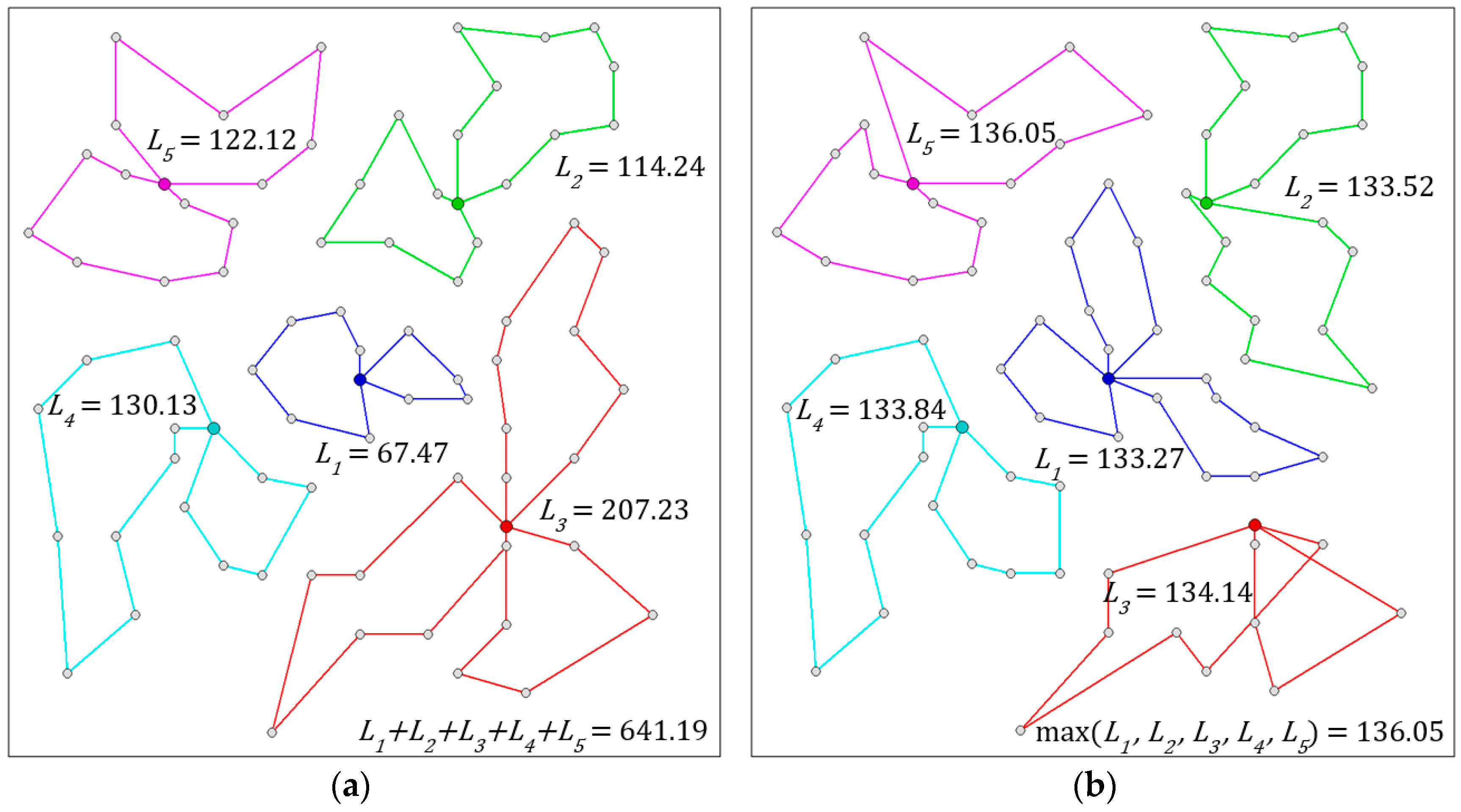
MDVRP is a problem where a set of customers should be served by a fleet of vehicles originating from multiple depots. Each customer is served (visited) just once by any vehicle in a fleet. Every vehicle visits a number of customers in a certain order along its route, and then returns to its depot.

The optimization criterion of MDVRP is to minimize the total sum of distances traveled by all vehicles in a fleet, according to Formula (1).

$$\mathrm{mimimize}({{\displaystyle \sum }}_{i=1}^N{D}_i),$$

(1)

where $D_i$ is the distance travelled by $i$-th vehicle in the fleet, $N$ is the total number of vehicles.

The standard formulation of MDVRP can be broadened by introducing a capacity constraint. Each customer requires some amount of load to be delivered by a vehicle; the maximum load of each vehicle is then specified. If the following customer on the route would exceed the maximum load, the vehicle must return to its depot before continuing to this customer. A similar constraint can be set by limiting the maximum length of each route.

3.1. Modification

The modified version of MDVRP presented in this article (hereafter referred to as M-MDVRP) alters the optimization criterion. The objective of the task is not to minimize the total distance traveled, but to minimize the longest route of all vehicles in the fleet according to Formula (2). Moreover, the length of each route can be understood not only as the distance of this route, but also as the time necessary for a vehicle to take this route. The importance of using time instead of distance is in tasks where average velocities of individual vehicles are not the same.

$$\mathrm{mimimize}\left(\max \left(L_1,L_2,\dots ,L_N\right)\right),$$

(2)

where $L_i$ is the length of the route of $i$-th vehicle in the fleet, and $N$ is the total number of vehicles (routes).

The modification of the optimization criterion does not affect the NP-hardness of the problem. To prove this, the reduction from the well-known NP-complete decision version of the Hamiltonian Cycle to the M-MDVRP can be performed in polynomial time, according to the same principles as those presented in [28].

3.2. Impact of the Modified Criterion

The difference between MDVRP and M-MDVRP is illustrated on Cordeau’s benchmark instance p03 [29,30]. This instance is composed of 75 randomly distributed customers and a fleet of five vehicles.

Table 1. Difference between MDVRP and M-MDVRP shown on instance p03.

Problem	BKS	ACO	Gap
MDVRP	(a) 641.19	(c) 670.82	(e) 4.62%
M-MDVRP	(b) 207.23	(d) 136.05	(f) 52.32%

presents the best known solution (BKS) for this task [31]—see value (a). This solution was found using the optimization criterion from Formula (1). Value (b) in the same column shows the same solution (set of routes); the cost, however, is recalculated according to the modified criterion specified in Formula (2). The third column shows the result found using the ACO algorithm proposed by the author (for details see Section 4). Value (d) presents the best solution found for this instance and modified criterion, whereas value (c) is the same solution recalculated in a similar way to the previous case, i.e., for the opposite criterion (1). Values (e) and (f) in the last column in Table 1 show the differences (gaps) between solutions (a) and (c), and (d) and (b) respectively. However, these values cannot be used to compare the quality of the algorithms, because different criteria were used for optimization.

Figure 1 shows the situation graphically. On the left is the solution for the MDVRP optimization criterion, on the right the solution for M-MDVRP. Routes for individual vehicles are color coded. As can be seen, a vehicle may return to its depot several times on its route because the capacity and/or route length constraints exist. The lengths for all routes are also shown. The sum of these values serve as the solution for MDVRP, and the biggest value serves as the solution for M-MDVRP. Note the similar lengths in Figure 1b; the burden of serving customers is thus distributed to individual vehicles as equally as possible.

4. Metaheuristic Solution

This section introduces the metaheuristic algorithm proposed by the author for finding both MDVRP and M-MDVRP solutions. The algorithm also takes into consideration the capacity and route length constraints. It is also suitable for asymmetric and/or oriented graphs. Moreover, different vehicles in the fleet can be assigned different velocities.

This section presents only the basic features of the original algorithm, as details have already been published [32]. More attention is paid to the as yet unpublished additional optimization process, which enhances the original metaheuristic algorithm by a deterministic approach.

4.1. Original Algorithm

The algorithm is a probabilistic technique for solving computational problems. It is an example of a swarm intelligence method. The principle is adopted from the natural world, where ants explore their environment to find food. The exploring starts randomly at first; when an ant finds food, however, it lays down a pheromone trail along its route. When other ants find such trail, they are likely to follow it (and lay down their own trail if successful).

Figure 2 shows a flowchart with the basic phases of the ACO algorithm. As the approach is metaheuristic, the search space is explored in a finite number of iterations. The algorithm works with the number of ants. In each iteration, a solution is found for each ant via the heuristic approach, which involves the cost between nodes and the strength of pheromone trails (phase ①).

Phase ② represents the additional optimization process applied only to the best solution in a current iteration. It is launched when the specific condition is met (see Section 4.2). In phase ③, pheromone trails evaporate gradually to avoid convergence to a locally optimal solution, and then they are updated according to the best solution found in the current iteration. Unless the termination condition is met, the next iteration starts.

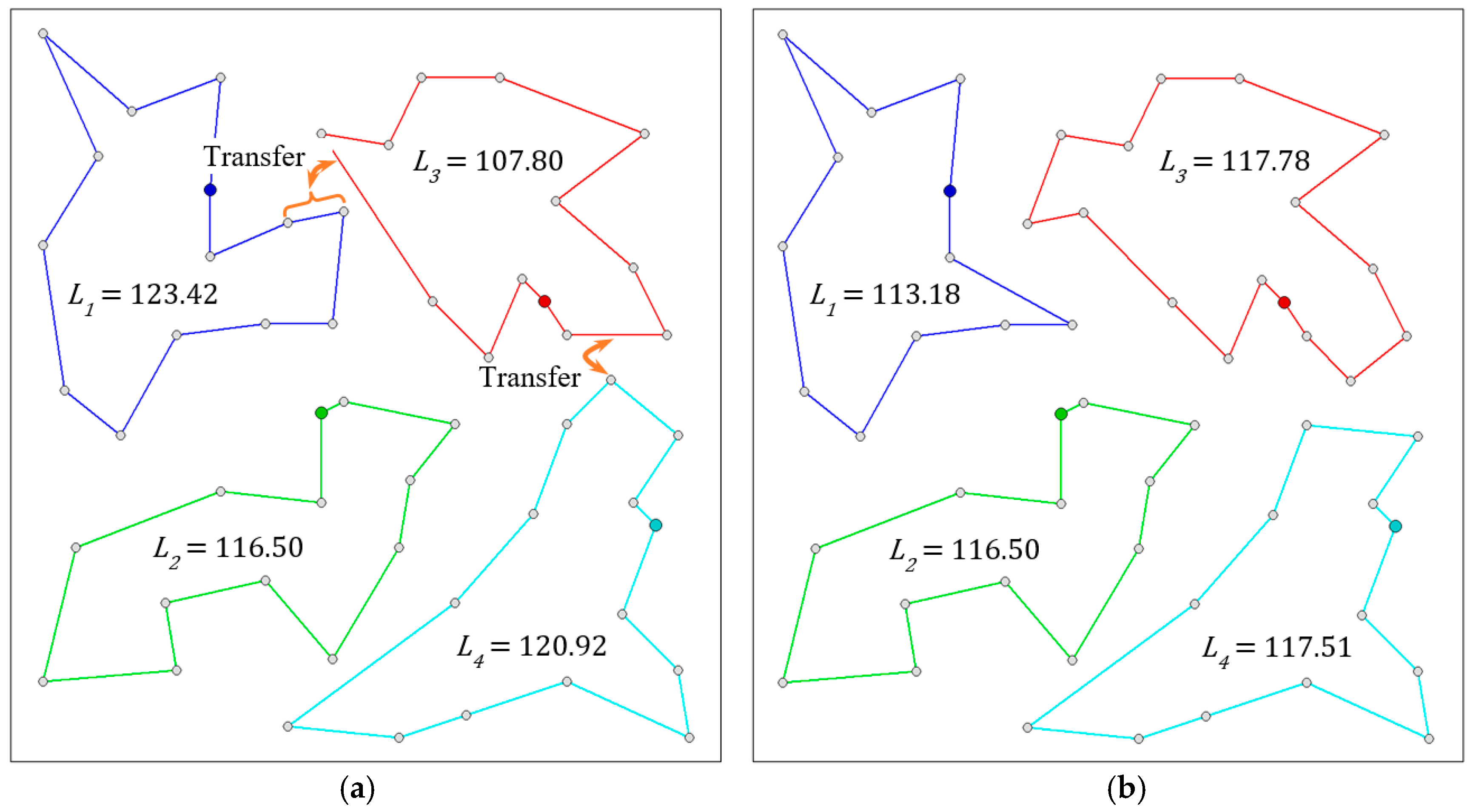
4.2. Additional Optimization Process

The additional optimization process (AOP) is executed depending on the repetition frequency coefficient. It was found empirically that the best values of the repetition frequency vary from 5 to 10; values lower than 5 mean faster convergence to a locally optimal solution. AOP is applied only for the best solution found within an iteration (see phase ① in Figure 2) in order to further improve the solution, which is then used for updating the pheromone trails (see phase ③ in Figure 2).

AOP is a deterministic approach which incorporates two independent steps as follows:

• Single route optimization (SRO),
• Mutual routes optimization (MRO).

SRO is launched for each route separately. It is based on the consecutive identification of nodes to be exchanged within every route. As a result of the exchange, a new solution is created and evaluated. If it surpasses the original solution, the new solution replaces the original.

This process is shown in pseudocode in Algorithms 1. Variable $n$ represents the number of nodes to be replaced. It starts from 1 and continues to $n_{max}$; it was found empirically that $n_{max}$ does not have to be bigger than 2. If $n>1$, then $n$ successive nodes are selected. In this way, all possible combinations of $n$ successive nodes are removed and placed to all different possible positions on the route.

Algorithms 1. Single route optimization in pseudocode.

The principle is illustrated in Figure 3 in an example with 50 nodes and 4 vehicles. The lengths of individual routes are displayed. Figure 3a shows the situation before the SRO. The nodes identified for exchange are indicated on the blue route. Figure 3b shows the situation after the SRO, where these nodes are replaced on the routes, i.e., the order of nodes to be visited by the vehicles is changed. As a result, the quality of this new solution was improved from 138.65 to 123.42.

While the SRO finds a better solution by replacing nodes belonging to the same route, MRO incorporates a similar process for nodes from different routes. During this process, nodes to be transferred from one route to another are identified for every combination of pairs of routes. This process is shown in pseudocode in Algorithms 2. It is executed independently for all possible pairs (combinations) of routes.

The principle of MRO is illustrated in Figure 4. It uses the solution obtained after SRO was applied (see Figure 3b). In Figure 4a, nodes identified for removal from the blue and azure routes are emphasized. These nodes are then inserted into the red route. Consequently, the quality of this new solution was further improved from 123.42 to 117.78.

Algorithms 2. Mutual routes optimization in pseudocode.

Each newly created route in the SRO process replaces the original, provided that the new route is better than the original, i.e., its length is shorter according to Formula (3).

$$L_{new}^i<L_{orig}^i,$$

(3)

where $L_{orig}^i$ is the length of the original route, $L_{new}^i$ is the length of the newly created route, $i$ identifies a route in the solution ($i=1\mathrm{to}M$ where $M$ is the number of vehicles/routes).

In the MRO process, the acceptance criterion depends on the type of problem. For MDVRP, when the total distance is minimized, the two newly created routes influenced by the process replace the originals when either Formula (4) or (5) are satisfied. The choice of formula depends on the setting of the algorithm. For M-MDVRP, when the longest route is minimized, Formula (6) must be satisfied.

$$L_{new}^i<L_{orig}^i\mathrm{and}{L}_{new}^j<L_{orig}^j,$$

(4)

$$L_{new}^i+L_{new}^j<L_{orig}^i+L_{orig}^j,$$

(5)

$$\max (L_{new}^i,L_{new}^j)<\max (L_{orig}^i,L_{orig}^j),$$

(6)

where $L_{orig}^i$ and $L_{orig}^j$ are the lengths of the original pair of routes, $L_{new}^i$ and $L_{new}^j$ are the lengths of the newly created pair of routes, $i$ and $j$ identify routes in the solution ($i,j=1\mathrm{to}M$; $i\ne j$).

5. Experiments and Results

Cordeau’s benchmark instances [29,30] were used for the experiments. At first, the comparison of the original ACO algorithm with this algorithm enhanced by the additional optimization process was conducted; the parameters and settings of the algorithms were the same. The modified optimization criterion was used in experiments.

Table 2. Comparison of the ACO algorithm with and without AOP process.

Instance	Original ACO	Orig. ACO Runtime	ACO with AOP	ACO AOP Runtime	Solution Gap	Runtime Gap
p01	157.31	1.5 s	152.54	1.7 s	3.13%	11.11%
p02	129.00	1.6 s	125.82	1.8 s	2.53%	14.58%
p03	139.66	3.7 s	136.05	4.3 s	2.65%	16.22%
p04	518.37	23.1 s	511.41	28.4 s	1.36%	22.94%
p05	381.99	20.7 s	378.17	25.6 s	1.01%	23.83%
p06	314.87	25.7 s	301.75	31.9 s	4.35%	24.25%
p07	248.07	25.2 s	228.95	30.9 s	8.35%	22.75%
p08	2480.46	233.1 s	2224.85	361.0 s	11.49%	54.85%
p09	1468.86	267.3 s	1364.70	418.3 s	7.63%	56.49%
p10	1055.09	301.0 s	960.76	468.5 s	9.82%	55.65%
p11	795.28	278.5 s	749.41	422.9 s	6.12%	51.85%
p12	663.04	12.8 s	659.48	15.4 s	0.54%	20.58%
p13	659.48	13.4 s	659.48	16.0 s	0.00%	19.59%
p14	682.84	14.2 s	682.84	16.9 s	0.00%	18.86%
p15	730.20	124.6 s	640.58	167.1 s	13.99%	34.08%
p16	788.12	138.0 s	651.55	188.1 s	20.96%	36.28%
p17	817.65	111.4 s	677.27	147.3 s	20.73%	32.26%
p18	761.92	188.9 s	652.24	279.2 s	16.82%	47.79%
p19	870.90	175.3 s	651.55	253.1 s	33.67%	44.40%
p20	916.53	200.3 s	681.13	292.8 s	34.56%	46.18%
p21	862.00	466.0 s	659.25	818.8 s	30.75%	75.70%
p22	962.17	506.2 s	657.90	952.4 s	46.25%	88.14%
p23	1010.87	488.5 s	686.69	895.2 s	47.21%	83.25%

shows the results. As can be seen, the AOP process yielded considerably improved solutions. In 21 out of 23 cases, the solutions have been improved. In the remaining cases (p13, p14), the solutions are the same. Since these are the simplest instances with 80 regularly distributed nodes, it can be assumed that these solutions are optimal. In general, the more complex the problem, the higher the level of improvement. The average improvement over all 23 instances is 14.08%.

Table 2 also shows the average runtime of one execution of both the original ACO and the ACO with AOP for every instance. All experiments were carried out on a computer with the following configuration: Intel i7 4 GHz CPU with 8 cores, 16 GB RAM, operating system Windows 10. The codes of the algorithms were written in C++ in the Visual Studio IDE. As can be seen, the AOP process requires some extra time, which depends on the complexity of the problem, i.e., the number of nodes. For problems with 360 nodes (p21, p22, p23), the time required to obtain a solution with the algorithm with AOP was about 80% longer compared to the original ACO. Overall, the increase of the runtime on all Cordeau’s benchmark instances is 39.2%.

Table 3. Experiments.

Instance (N/M)	Problem	BKS	ACO	Gap
p01 (50/4)	MDVRP	576.87	607.66	5.34%
	M-MDVRP	237.81	152.54	55.90%
p02 (50/4)	MDVRP	473.53	495.34	4.61%
	M-MDVRP	169.57	125.82	34.77%
p03 (75/5)	MDVRP	641.19	670.82	4.62%
	M-MDVRP	207.23	136.05	52.32%
p04 (100/2)	MDVRP	1001.59	1021.36	1.97%
	M-MDVRP	532.24	511.41	4.07%
p05 (100/2)	MDVRP	750.03	750.72	0.09%
	M-MDVRP	378.17	378.17	0.00%
p06 (100/3)	MDVRP	876.50	902.91	3.01%
	M-MDVRP	432.59	301.75	43.36%
p07 (100/4)	MDVRP	885.80	907.55	2.46%
	M-MDVRP	246.21	228.95	7.54%
p08 (249/2)	MDVRP	4437.68	4449.65	0.27%
	M-MDVRP	2474.82	2224.85	11.24%
p09 (249/3)	MDVRP	3900.22	4085.51	4.75%
	M-MDVRP	1836.00	1364.70	34.54%
p10 (249/4)	MDVRP	3663.02	3825.73	4.44%
	M-MDVRP	1049.12	960.76	9.20%
p11 (249/5)	MDVRP	3554.18	3732.36	5.01%
	M-MDVRP	808.21	749.41	7.85%
p12 (80/2)	MDVRP	1318.95	1318.95	0.00%
	M-MDVRP	659.48	659.48	0.00%
p13 (80/2)	MDVRP	1318.95	1318.95	0.00%
	M-MDVRP	659.48	659.48	0.00%
p14 (80/2)	MDVRP	1360.12	1365.69	0.41%
	M-MDVRP	686.69	682.84	0.56%
p15 (160/4)	MDVRP	2505.42	2554.12	1.94%
	M-MDVRP	646.92	640.58	0.99%
p16 (160/4)	MDVRP	2572.23	2606.22	1.32%
	M-MDVRP	694.27	651.55	6.56%
p17 (160/4)	MDVRP	2709.09	2709.09	0.00%
	M-MDVRP	690.55	677.27	1.96%
p18 (240/6)	MDVRP	3702.85	3871.01	4.54%
	M-MDVRP	895.50	652.24	37.30%
p19 (240/6)	MDVRP	3827.06	3884.81	1.51%
	M-MDVRP	694.27	651.55	6.56%
p20 (240/6)	MDVRP	4058.07	4058.07	0.00%
	M-MDVRP	690.55	681.13	1.38%
p21 (360/9)	MDVRP	5474.84	5824.58	6.39%
	M-MDVRP	936.62	659.25	42.07%
p22 (360/9)	MDVRP	5702.16	5873.41	3.00%
	M-MDVRP	719.64	657.90	9.38%
p23 (360/9)	MDVRP	6095.46	6124.67	0.48%
	M-MDVRP	690.55	686.69	0.56%

presents the results in the same manner as Table 1. For each instance, numbers of nodes (N) and depots (M) are shown. The numbers in bold in the third column record the best known solutions (BKS) taken from NEO Web [31] (available at http://neo.lcc.uma.es/vrp/vrp-instances/multiple-depot-vrp-instances/), i.e., the MDVRP optimization criterion (Formula (1)) was used.

The ACO algorithm (with AOP process) was executed 100 times on each instance; the best solution is recorded in the fourth column of Table 3 (numbers in bold), with the M-MDVRP optimization criterion applied (Formula (2)). Both BKS and ACO solutions were then recalculated using the opposite optimization criterion, i.e., BKS solutions with the M-MDVRP criterion, and vice versa. All solutions from Table 3 are available for download at http://www.unob.cz/en/fml/structure/k110/m-mdvrp.

The difference (gap) between BKS and ACO solutions (both for MDVRP and M-MDVRP optimization criteria) are also shown in the last column of Table 3. These values do not indicate the quality of the algorithms, because different optimization criteria were used for optimization.

The quality of results in Table 3 can be estimated by comparing the lengths of individual routes within the solution, since this indicates the distribution of the delivery process to individual vehicles; the smaller the differences between the routes, the better the solution.

Table 4. Comparison of lengths of routes for solutions of benchmark instances.

Instance	Routes (Solution in Bold)	AvgDev (%)	StDev (%)
p01	152.24|151.86|151.02|152.54	0.477 (0.31%)	0.661 (0.43%)
p02	125.15|125.47|125.82|118.90	2.469 (1.96%)	3.303 (2.63%)
p03	133.27|133.52|134.14|133.84|136.05	0.754 (0.55%)	1.104 (0.81%)
p04	511.41|509.95	0.732 (0.14%)	1.035 (0.20%)
p05	378.17|372.55	2.808 (0.74%)	3.971 (1.05%)
p06	301.02|300.14|301.75	0.551 (0.18%)	0.802 (0.27%)
p07	228.95|224.81|226.79|227.00	1.088 (0.48%)	1.695 (0.74%)
p08	2224.81|2224.85	0.020 (0.00%)	0.028 (0.00%)
p09	1364.70|1362.17|1358.63	2.134 (0.16%)	3.047 (0.22%)
p10	957.14|960.76|949.74|958.09	3.347 (0.35%)	4.720 (0.49%)
p11	741.42|747.49|749.41|748.34|745.70	2.328 (0.31%)	3.133 (0.42%)
p12	659.48|659.48	0.000 (0.00%)	0.000 (0.00%)
p13	659.48|659.48	0.000 (0.00%)	0.000 (0.00%)
p14	682.84|682.84	0.000 (0.00%)	0.000 (0.00%)
p15	638.15|640.58|636.12|639.28	1.398 (0.22%)	1.891 (0.30%)
p16	651.55|651.55|651.55|651.55	0.000 (0.00%)	0.000 (0.00%)
p17	677.27|677.27|677.27|677.27	0.000 (0.00%)	0.000 (0.00%)
p18	646.11|641.43|647.94|652.24|650.51|632.78	5.375 (0.82%)	7.135 (1.09%)
p19	645.53|643.08|650.47|649.13|651.55|645.04	2.917 (0.45%)	3.387 (0.52%)
p20	667.85|677.27|677.27|681.13|677.27|677.27	2.831 (0.42%)	4.437 (0.65%)
p21	659.25|638.74|635.47|637.61|644.01|653.75|644.89|655.23|655.63	7.814 (1.19%)	8.948 (1.36%)
p22	653.49|656.33|655.88|643.55|643.08|657.90|652.34|654.27|656.57	4.185 (0.64%)	5.530 (0.84%)
p23	675.58|683.13|677.27|679.28|673.42|686.69|681.15|683.13|685.00	3.671 (0.53%)	4.460 (0.65%)

shows the average and standard deviation for all benchmark instances. As an example, the standard deviation for benchmark instance p09 is 3.047, which is 0.22% of the solution. The mean of the average deviation values is 0.41% and of the standard deviation values 0.55%.

The principle of estimating the quality of solutions by computing the standard deviation is shown in

Table 5. Comparison of lengths of routes for various solutions.

Instance	BKS	Original ACO	ACO with AOP
	StDev (%)	StDev (%)	StDev (%)
p01	75.912 (31.92%)	3.547 (2.25%)	0.661 (0.43%)
p02	35.989 (21.22%)	3.040 (2.36%)	3.303 (2.63%)
p03	50.421 (24.33%)	0.667 (0.48%)	1.104 (0.81%)
p04	44.466 (8.35%)	0.743 (0.14%)	1.035 (0.20%)
p05	4.457 (1.18%)	0.605 (0.16%)	3.971 (1.05%)
p06	122.020 (28.21%)	2.761 (0.88%)	0.802 (0.27%)
p07	21.018 (8.54%)	9.725 (3.92%)	1.695 (0.74%)
p08	9.393 (0.42%)	3.486 (0.14%)	0.028 (0.00%)
p09	480.583 (26.18%)	8.838 (0.60%)	3.047 (0.22%)
p10	114.528 (10.92%)	3.722 (0.35%)	4.720 (0.49%)
p11	96.537 (11.94%)	24.424 (3.07%)	3.133 (0.42%)
p12	0.000 (0.00%)	0.000 (0.00%)	0.000 (0.00%)
p13	0.000 (0.00%)	0.000 (0.00%)	0.000 (0.00%)
p14	9.385 (1.37%)	0.000 (0.00%)	0.000 (0.00%)
p15	23.746 (3.67%)	20.894 (2.86%)	1.891 (0.30%)
p16	59.136 (8.52%)	5.189 (0.66%)	0.000 (0.00%)
p17	10.837 (1.57%)	24.148 (2.95%)	0.000 (0.00%)
p18	209.406 (23.38%)	31.286 (4.11%)	7.135 (1.09%)
p19	46.958 (6.76%)	22.779 (2.62%)	3.387 (0.52%)
p20	11.839 (1.71%)	35.761 (3.90%)	4.437 (0.65%)
p21	199.647 (21.32%)	41.186 (4.78%)	8.948 (1.36%)
p22	69.188 (9.61%)	60.946 (6.33%)	5.530 (0.84%)
p23	9.598 (1.39%)	80.569 (7.97%)	4.460 (0.65%)

, which compares these values for the BKS solutions (see Table 3) and solutions obtained by the original ACO algorithm and the ACO algorithm with AOP (see Table 2). As can be seen, the values of the standard deviation are higher in most cases, for worse solutions. The mean of the standard deviation for the BKS solutions is 10.98%, 2.20% for the solutions of the original ACO, and 0.55% for the solutions of the ACO with AOP.

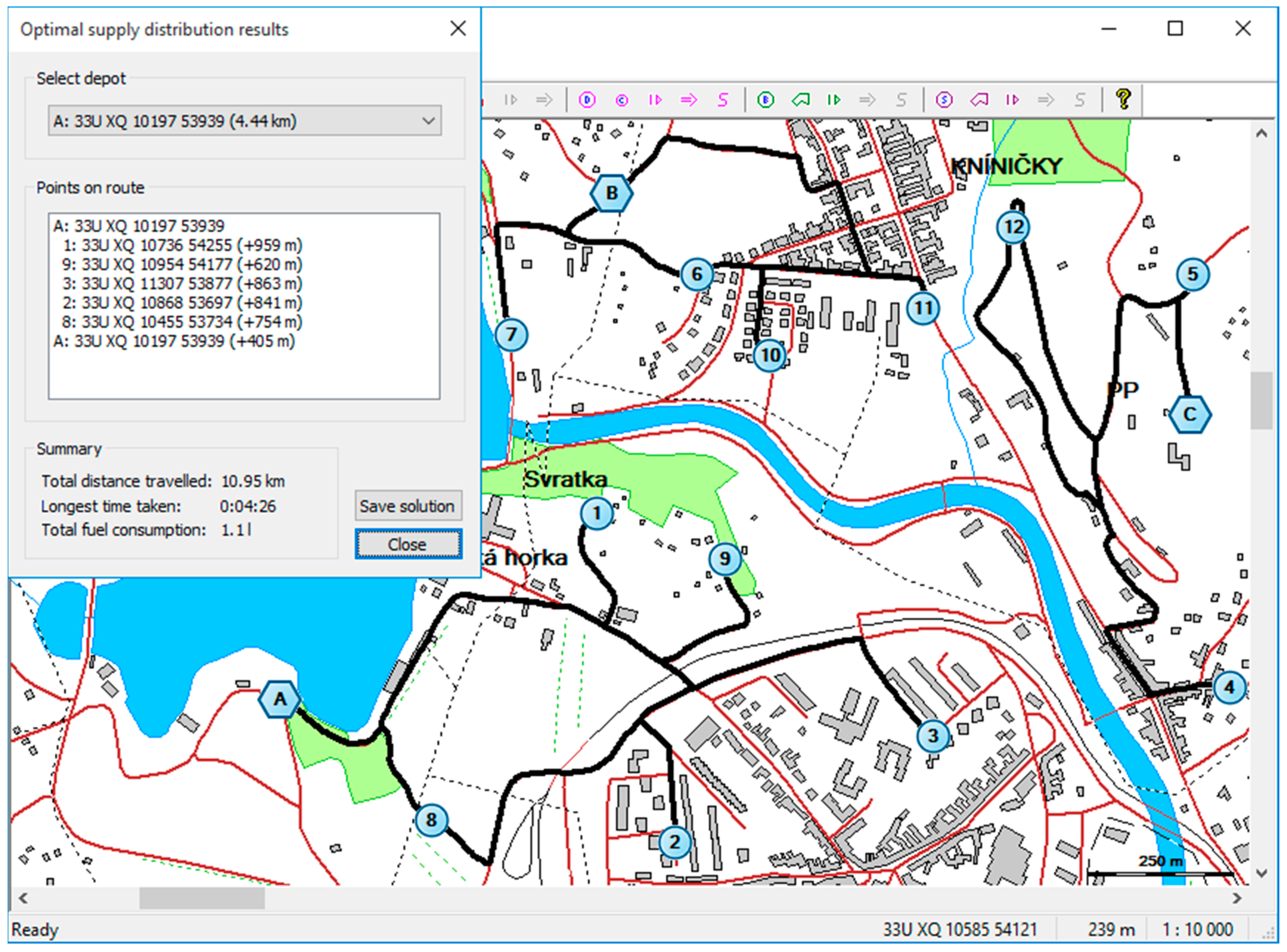
6. Practical Application

The proposed algorithm is utilized in the Tactical Decision Support System (TDSS) being developed at the University of Defense, Czech Republic. TDSS aims at supporting commanders of the Czech Army in their decision-making at the tactical level. It has been implemented into several models of military tactics, such as optimal cooperative reconnaissance by aerial and/or ground unmanned vehicles, and optimal logistics distribution on the battlefield. More details about the information support of commanders can be found in [33,34,35,36,37,38,39].

An example of the optimal logistics distribution model is shown in Figure 5. In this model, units (see blue circles labeled by numbers) deployed in the area of operations are supplied by logistic vehicles (see blue hexagons labeled by letters). Each unit may have different requirements for the amount of supplies it needs; the maximum capacity constraint of the supplying vehicles is thus taken into account. The model plans the entire logistic operation: each supplying vehicle knows the order of units it needs to visit and the shortest routes between them (see the black thick lines in Figure 5).

The modified optimization criterion defined in Formula (2) is used mostly in this problem, as the general requirement is to conduct the operation as quickly as possible. Alternatively, the optimization criterion to minimize the fuel consumed can be selected. In such a case, the cost of an edge in the graph is computed as the fuel consumed by a vehicle which moves along the route between the nodes connecting the edge. This creates an asymmetric graph as the fuel consumed by moving between two nodes may differ, depending on the direction of travel; this is however no limitation for the proposed algorithm. More information about this model can be found in [33].

7. Conclusions

This article presents the Multi-Depot Vehicle Routing Problem with a modified optimization criterion. This problem is known as Min-Max MDVRP in the literature. The first part of the paper shows the impact of the modification compared to the standard MDVRP.

For solving modified MDVRP, the Ant Colony Optimization principle was used. The original algorithm published by the author in [32] was adapted and modified for M-MDVRP. Moreover, this algorithm was enhanced by a deterministic optimization process which is executed repeatedly within the iterations of the ACO algorithm. This process improved the results considerably, as can be seen from Table 2; the average improvement over all 23 benchmark instances is 14.08%.

For an evaluation of M-MDVRP solutions, Cordeau’s benchmark instances were used. For each instance, two solutions exist: the solution found by the ACO algorithm (using modified MDVRP criterion), and the best known solution, taken from the literature (using standard MDVRP criterion). Both solutions are then recalculated using the opposite criterion: the solution found by the ACO algorithm is recalculated using the standard MDVRP criterion, and vice versa. As is obvious from Table 3, all solutions found by the ACO algorithm are better than the BKS solutions recalculated according to the modified criterion.

The quality of the ACO algorithm is then estimated by computing the average and standard deviation from individual routes of a solution. The quality is estimated under the assumption that the smaller the differences between individual routes, the better the quality of the solution. A solution where all the routes are of similar length ensures the balanced distribution of the delivery process to individual vehicles. The mean of the standard deviation computed from all solutions is only 0.55% of the lengths of the longest routes.

References

1. Dantzig, G.B.; Ramser, J.H. The truck dispatching problem. Manag. Sci. 1959, 6, 80–91. [Google Scholar] [CrossRef]
2. Carlsson, J.; Ge, D.; Subramaniam, A.; Wu, A.; Ye, Y. Solving min-max multi-depot vehicle routing problem. Lect. Glob. Optim. 2009, 55, 31–46. [Google Scholar]
3. Narasimha, K.V.; Kivelevitch, E.; Sharma, B.; Kumar, M. An ant colony optimization technique for solving min–max multi-depot vehicle routing problem. Swarm Evolut. Comput. 2013, 13, 63–73. [Google Scholar] [CrossRef]
4. Ho, W.; Ho, G.T.S.; Ji, P.; Lau, H.C.W. A hybrid genetic algorithm for the multi-depot vehicle routing problem. Eng. Appl. Artif. Intell. 2008, 21, 548–557. [Google Scholar] [CrossRef]
5. Sharma, N.; Monika, M.A. Literature Survey on Multi-Depot Vehicle Routing Problem. Int. J. Res. Dev. 2015, 3, 1752–1757. [Google Scholar]
6. Montoya-Torres, J.R.; Franco, J.L.; Isaza, S.N.; Jiménez, H.F.; Herazo-Padilla, N. A literature review of the vehicle routing problem with multiple depots. Comput. Ind. Eng. 2015, 79, 115–129. [Google Scholar] [CrossRef]
7. Braekers, K.; Ramaekers, K.; Van Nieuwenhuyse, I. The vehicle routing problem: State of the art classification and review. Comput. Ind. Eng. 2016, 99, 300–313. [Google Scholar] [CrossRef]
8. Gillett, B.E.; Johnson, J.G. Multi-terminal vehicle-dispatch algorithm. Omega 1976, 4, 711–718. [Google Scholar] [CrossRef]
9. Chao, M.I.; Golden, B.L.; Wasil, E. A new heuristic for the multi-depot vehicle routing problem that improves upon best-known solutions. Am. J. Math. Manag. Sci. 1993, 13, 371–406. [Google Scholar] [CrossRef]
10. Renaud, J.; Laporte, G.; Boctor, F.F. A tabu search heuristic for the multi-depot vehicle routing problem. Comput. Oper. Res. 1996, 23, 229–235. [Google Scholar] [CrossRef]
11. Escobar, J.W.; Linfati, R.; Toth, P.; Baldoquin, M.G. A hybrid Granular Tabu Search algorithm for the Multi-Depot Vehicle Routing Problem. J. Heuristics 2014, 20, 483–509. [Google Scholar] [CrossRef]
12. Soto, M.; Sevaux, M.; Rossi, A.; Reinholzc, A. Multiple neighborhood search, tabu search and ejection chains for the multi-depot open vehicle routing problem. Comput. Ind. Eng. 2017, 107, 211–222. [Google Scholar] [CrossRef]
13. Wu, T.H.; Low, C.; Bai, J.W. Heuristic solutions to multi-depot location routing problems. Comput. Oper. Res. 2002, 29, 1393–1415. [Google Scholar] [CrossRef]
14. Lim, A.; Zhu, W. A fast and effective insertion algorithm for multi-depot vehicle routing problem and a new simulated annealing approach. In Advances in Artificial Intelligence, Lecture Notes in Computer Science; Springer: Berlin/Heidelberg, Germany, 2006; Volume 4031, pp. 282–291. [Google Scholar]
15. Ombuki-Berman, B.; Hanshar, F.T. Using Genetic Algorithms for Multi-depot Vehicle Routing. In Bio-Inspired Algorithms for the Vehicle Routing Problem; Springer: Berlin/Heidelberg, Germany, 2009; Volume 161, pp. 77–99. [Google Scholar]
16. Seidgar, H.; Abedi, M.; Tadayoni, S.; Rezaeian, J. An efficient hybrid of genetic and simulated annealing algorithms for multi server vehicle routing problem with multi entry. Int. J. Ind. Syst. Eng. 2016, 24, 333–360. [Google Scholar] [CrossRef]
17. Karakatic, S.; Podgorelec, V. A survey of genetic algorithms for solving multi-depot vehicle routing problem. Appl. Soft Comput. 2015, 27, 519–532. [Google Scholar] [CrossRef]
18. Yu, B.; Yang, Z.Z.; Xie, J.X. A parallel improved ant colony optimization for multi-depot vehicle routing problem. J. Oper. Res. Soc. 2010, 62, 183–188. [Google Scholar] [CrossRef]
19. Yao, B.; Hu, P.; Zhang, M.; Tian, X. Improved Ant Colony Optimization for Seafood Product Delivery Routing Problem. Promet-Traffic Transp. 2014, 26, 1–10. [Google Scholar] [CrossRef]
20. Tang, Y. An Improved Ant Colony Optimization for Multi-Depot Vehicle Routing Problem. International. J. Eng. Technol. 2016, 8, 385–388. [Google Scholar]
21. Gao, J. Automobile chain maintenance parts delivery problem using an improved ant colony algorithm. Adv. Mech. Eng. 2016, 8, 1–13. [Google Scholar] [CrossRef]
22. Ma, Y.; Han, J.; Kang, K.; Yan, F. An Improved ACO for the Multi-depot Vehicle Routing Problem with Time Windows. In Proceedings of the Tenth International Conference on Management Science and Engineering Management; Advances in Intelligent Systems and Computing; Springer: Singapore, 2017; Volume 502. [Google Scholar]
23. Ting, C.J.; Chen, C.H. Combination of multiple ant colony system and simulated annealing for the multi-depot vehicle routing problem with time windows. Transp. Res. Rec. J. Transp. Res. Board 2008, 2089, 85–92. [Google Scholar] [CrossRef]
24. Vidal, T.; Crainic, T.G.; Gendreau, M.; Lahrichi, N.; Rei, W. A Hybrid Genetic Algorithm for Multi-Depot and Periodic Vehicle Routing Problems. Oper. Res. 2012, 60, 611–624. [Google Scholar] [CrossRef]
25. De Oliveira, F.B.; Enayatifar, R.; Sadaei, H.J.; Guimarães, F.G.; Potvin, J.Y. A cooperative coevolutionary algorithm for the Multi-Depot Vehicle Routing Problem. Expert Syst. Appl. 2016, 43, 117–130. [Google Scholar] [CrossRef]
26. Wang, X.; Golden, B.; Wasil, E. The min-max multi-depot vehicle routing problem: Heuristics and computational results. J. Oper. Res. Soc. 2015, 66, 1430–1441. [Google Scholar] [CrossRef]
27. Wang, X.; Golden, B.; Wasil, E.; Zhang, R. The min–max split delivery multi-depot vehicle routing problem with minimum service time requirement. Comput. Oper. Res. 2016, 71, 110–126. [Google Scholar] [CrossRef]
28. Benning, L. Why Is the Traveling Salesman Problem NP Complete? Quora.com. 2014. Available online: https://www.quora.com/Why-is-the-traveling-salesman-problem-NP-complete (accessed on 10 May 2018).
29. Cordeau, J.F.; Gendreau, M.; Laporte, G. A tabu search heuristic for periodic and multi-depot vehicle routing problems. Networks 1997, 30, 105–119. [Google Scholar] [CrossRef]
30. Cordeau, J.F.; Maischberger, M. A parallel iterated tabu search heuristic for vehicle routing problems. Comput. Oper. Res. 2012, 39, 2033–2050. [Google Scholar] [CrossRef]
31. NEO Web, Networking and Emerging Optimization. University of Malaga, Spain. Available online: http://neo.lcc.uma.es/vrp/vrp-instances/multiple-depot-vrp-instances/ (accessed on 19 February 2018).
32. Stodola, P.; Mazal, J. Applying the Ant Colony Optimisation Algorithm to the Capacitated Multi-Depot Vehicle Routing Problem. Int. J. Bio-Inspir. Comput. 2016, 8, 228–233. [Google Scholar]
33. Stodola, P.; Mazal, J. Tactical Decision Support System to Aid Commanders in their Decision-Making. In Modelling and Simulation for Autonomous Systems; Springer: Cham, Switzerland, 2016; pp. 396–406. [Google Scholar]
34. Blaha, M.; Silinger, K. Application support for topographical-geodetic issues for tactical and technical control of artillery fire. Int. J. Circuits Syst. Signal Proc. 2018, 12, 48–57. [Google Scholar]
35. Hodicky, J. Standards to support military autonomous system life cycle. In Advances in Intelligent Systems and Computing; Springer: Cham, Switzerland, 2018; Volume 644, pp. 671–678. [Google Scholar]
36. Rybansky, M. Trafficability analysis through vegetation. In Proceedings of the International Conference on Military Technologies, Brno, Czech Republic, 31 May–2 June 2017; pp. 207–210. [Google Scholar]
37. Drozd, J. Analysis Results of the Military Observer Training System. Econ. Manag. 2016, 2016, 24–31. [Google Scholar]
38. Farlik, J.; Casar, J.; Stary, V. Simplification of missile effective coverage zone in air defence simulations. In Proceedings of the International Conference on Military Technologies, Brno, Czech Republic, 31 May–2 June 2017; pp. 733–737. [Google Scholar]
39. Hasilova, K.; Vališ, D. Non-parametric estimates of the first hitting time of Li-ion battery. Measurement 2018, 113, 82–91. [Google Scholar] [CrossRef]
Figure 1. Solutions for benchmark instance p03. (a) MDVRP (best known solution) (b) M-MDVRP (ACO algorithm).
Algorithms 11 00074 g001
Figure 2. Flowchart for the ACO algorithm.
Algorithms 11 00074 g002
Figure 3. Single route optimization principle. (a) Before SRO (b) After SRO.
Algorithms 11 00074 g003
Figure 4. Mutual routes optimization principle. (a) Before MRO (b) After MRO.
Algorithms 11 00074 g004
Figure 5. Optimal logistics distribution on the battlefield [33].
Algorithms 11 00074 g005