2.1. The Desired Dynamics Equation (DDE) Method
Consider the transfer function given by:
where
and
are unknown parameters. It can be transformed to the following state space form:
where
are the plant input and its derivatives;
is the plant output;
are the system states;
is a proper positive constant number; and
is the total disturbance.
The desired dynamic equation is as follows:
To reach Equation (3), the corresponding control law should be:
where
and
are the coefficient of the desired dynamic and are determined by the requirements of the control system; and
is the estimation of total disturbance
.
To obtain the estimation of total disturbance
, the following disturbance observer is used.
where
is the coefficient of the disturbance observer and indicates the speed of tracking disturbance; and
is an intermediate variable.
Equation (5) structures a disturbance observer. Equation (4) offers the control law to achieve the desired dynamic Equation (3). The disturbance observer estimates the total disturbance and compensates the systems to be the desired dynamic in real time and dynamically.
By substituting Equations (2), (3) and (5) into Equation (4), we can obtain
where
is the target value; and
is the error between the plant output and the target value. The detailed derivation is shown in
Appendix A.
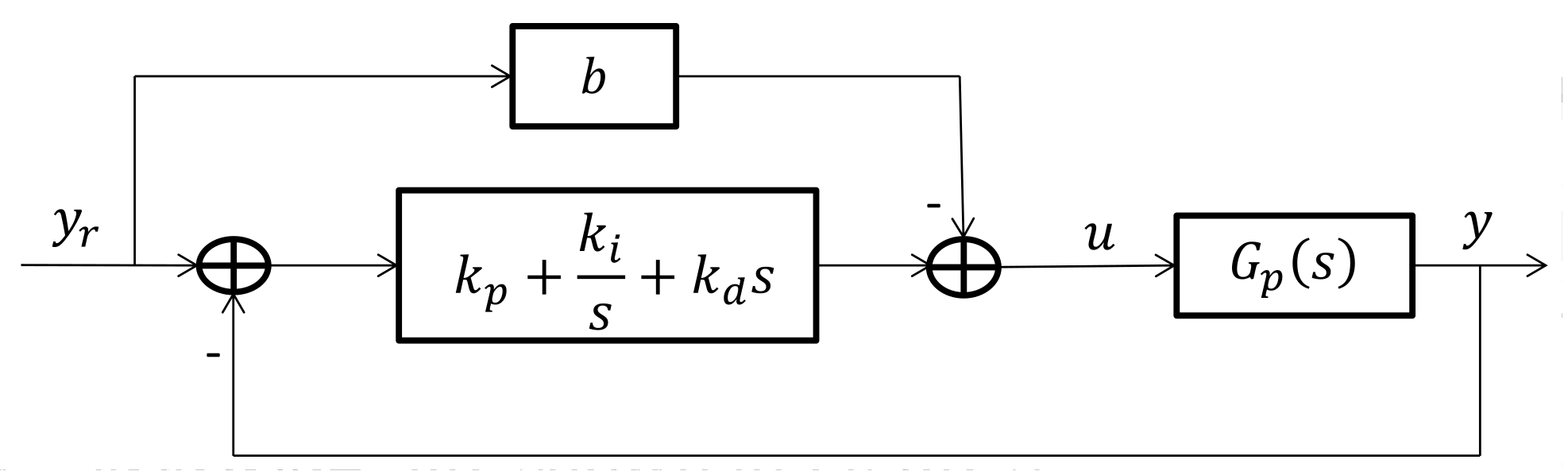
From Equation (6), we can obtain the two-degree-of-freedom PID controller parameters,
The corresponding two-degree-of-freedom PID controller structure is shown in
Figure 1.
When the desired dynamic equation is as follows:
we can analogously obtain the two-degree-of-freedom PID controller parameters,
In general, the DDE endows the 2-DOF PID controller parameters with clear physical meaning, which makes some of the parameters specified and then decreases the number of unknown parameters. Moreover, the model error is imposed into the total disturbance and is compensated, so the precise model is not necessary.
2.2. Generalized Frequency Method (GFM)
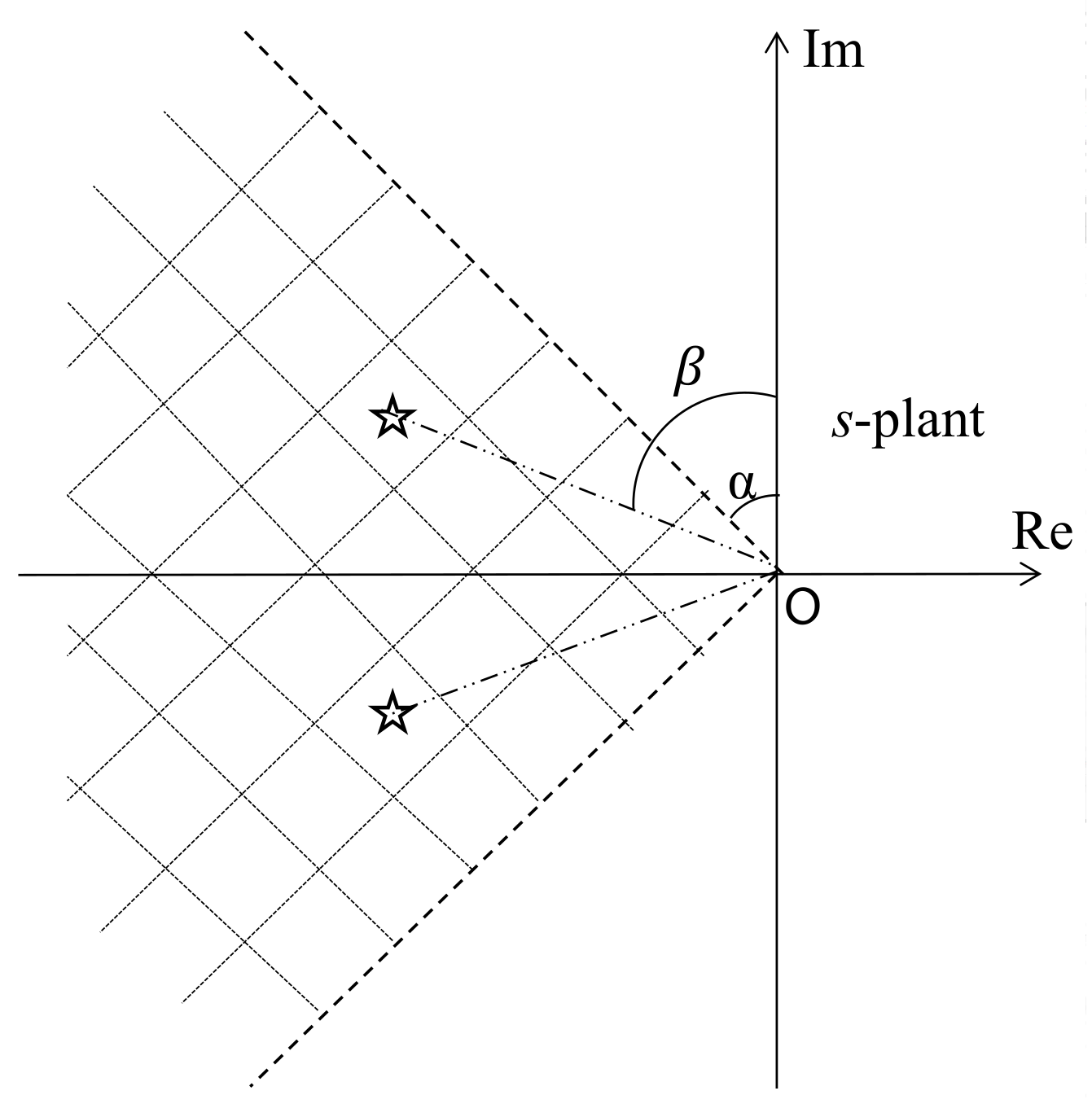
The GFM can calculate the controller parameters directly and analytically and can accurately guarantee the specified stability margin with only one parameter, which is called the attenuation index
. The attenuation index
determines the two rays, which shape a sector area shown in
Figure 2, and the GFM can make all the closed-loop poles lie in the resulting sector area. The equation of the two rays is
, where
,
.
is a constant and
is the included angle between the ray and the imaginary axis.
The stability margin increases with attenuation index . Each pair of conjugate complex poles have a corresponding , and the corresponding equal to infinity for the real poles. The minimum is equal to the specified attenuation index , i.e., .
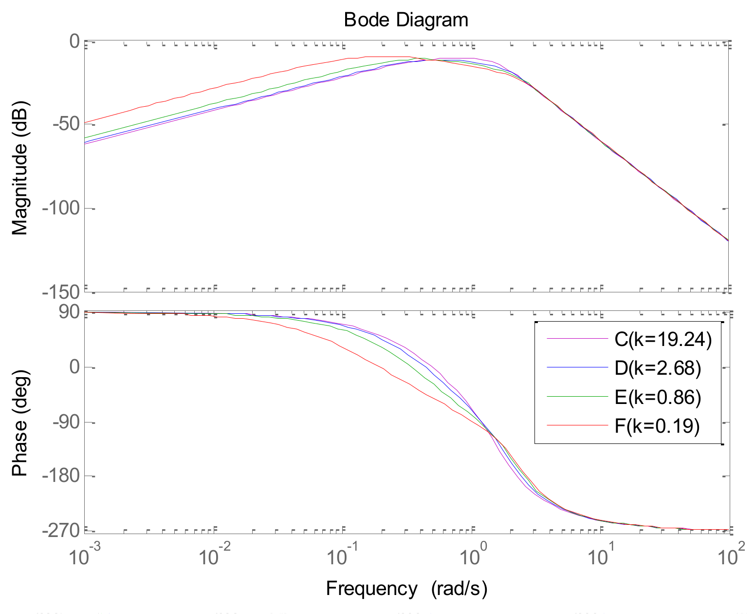
Next, we will illustrate the relationship between the maximum sensitivity (
) and the attenuation index
to explain the rationality of the attenuation index
as the stability margin criterion.
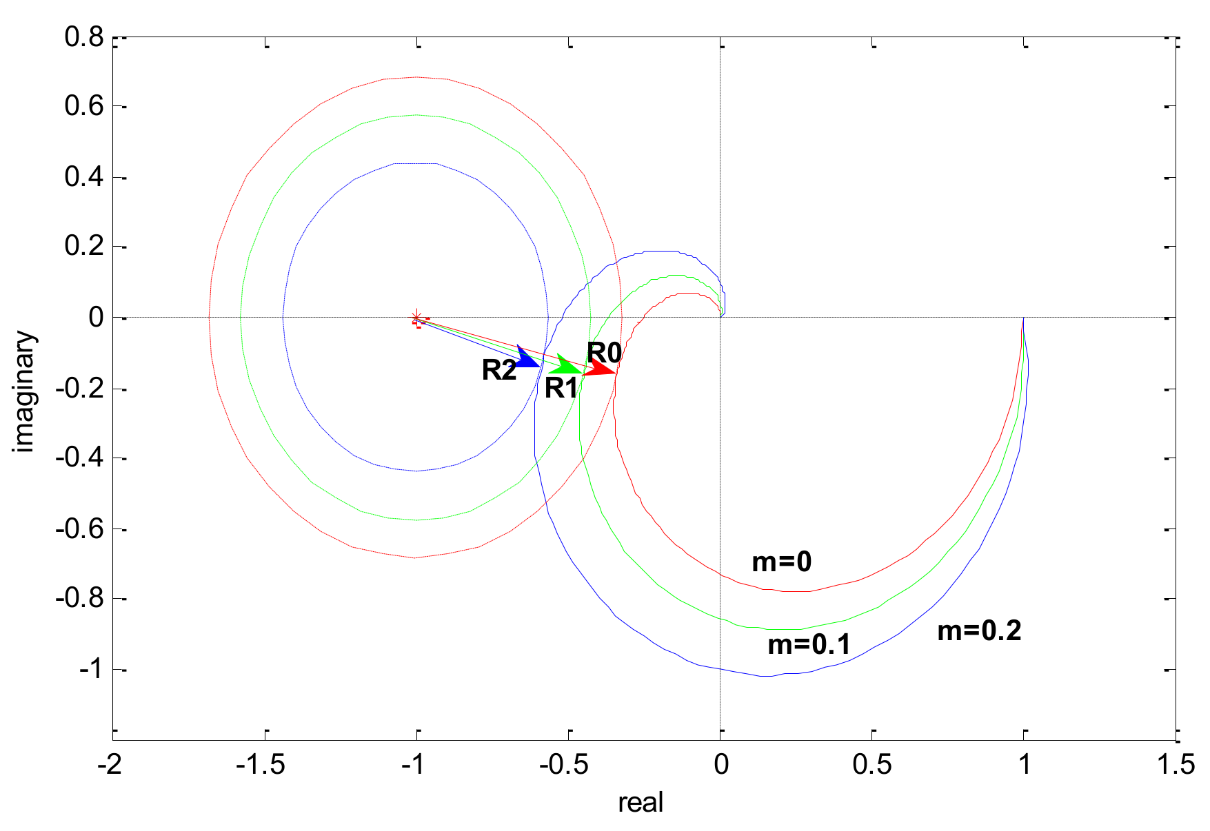
is taken as an example. Substitute
into
, and the Nyquist plots of
are shown in
Figure 3.
In
Figure 3, the Nyquist plots are shown with full lines, and
,
, and
are respectively shown with a red line, green line, and blue line; dashed lines represent the maximum sensitivity
and the dashed red line, green line, and blue line respectively represent
,
, and
. The stability margin of
decreases with the attenuation index
increasing. So, when designing the controller parameters, make the transfer function
to give
as the stability margin, where
represents the transfer function of the controller. From above, the attenuation index
can give a system stability margin in parameter design stage, and thus, it can be a stability margin criterion.
2.3. Setting PID Controllers Parameters
In this subsection, first a set of tuning equations is derived, and then, controller parameters are analyzed. Finally, the steps of the tuning method are given.
For the control system in
Figure 1, its stability is determined by the closed-loop characteristic equation:
Substitute
into Equation (10), define
, and compare the real and imaginary parts; the following equation is obtained
Under certain , Equation (11) structures a marginal stability surface with various . The marginal stability surface divides the space into two parts: meeting stability margin and not meeting stability margin.
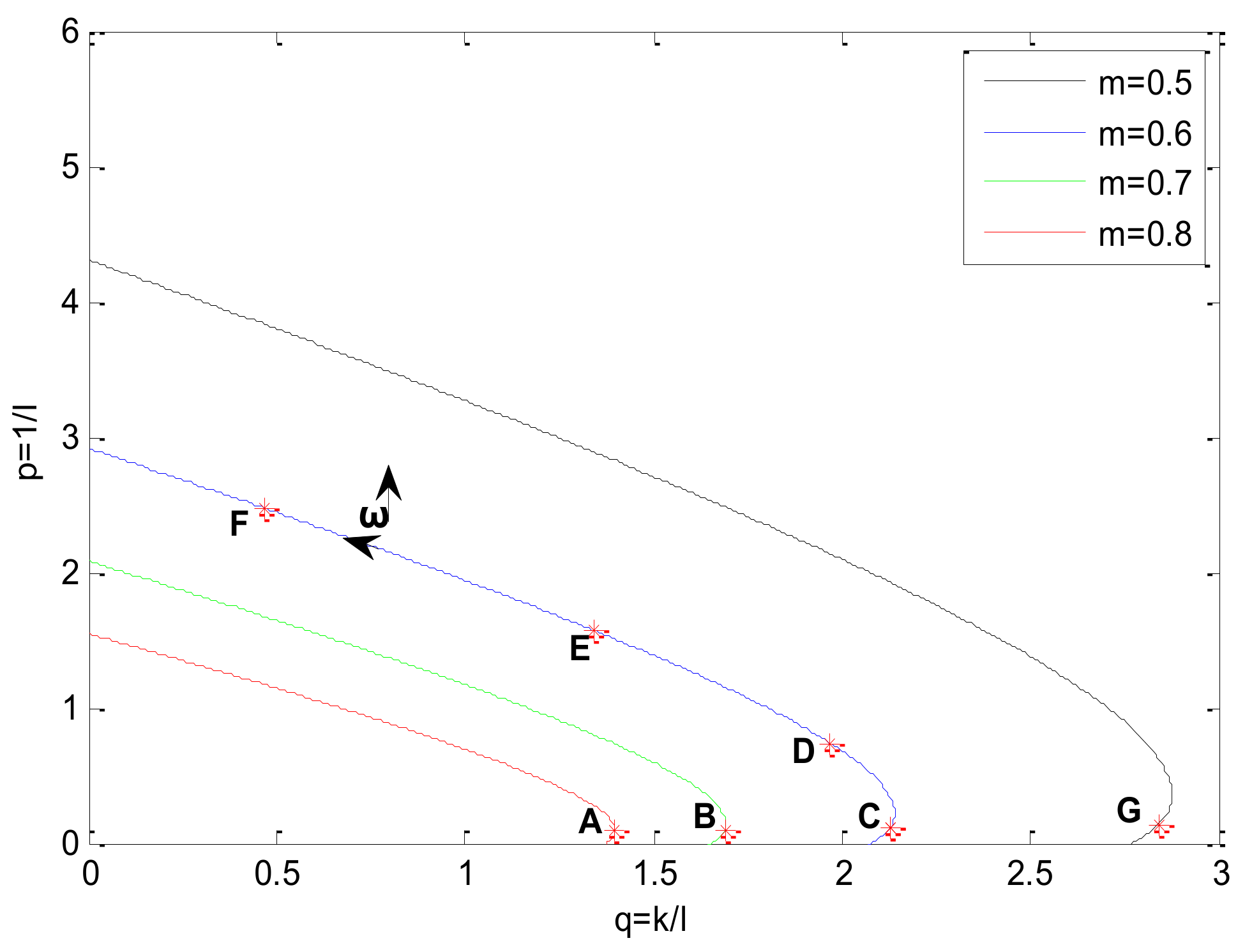
Employing the following variable substitution,
Equation (7) is expressed as
Substitute Equation (13) into Equation (11), and the following equation is obtained
Under certain , , and , Equation (14) becomes a linear equation. Then, if its Jacobian determinant J is nonsingular, it has a unique local solution . Under various and certain , and , Equation (14) has a unique local solution curve (i.e., marginal stability curve). The marginal stability curve divides the plane into two parts: meeting stability margin and not meeting stability margin. The curve is the contour. Then, once an appropriate work point in the contour is obtained, the controller parameters can be calculated. The method of choosing a work point is shown after the analysis of the parameter , because the parameter can influence the choosing method.
Next, the function of the controller parameters is analyzed, and the method for obtaining them is shown.
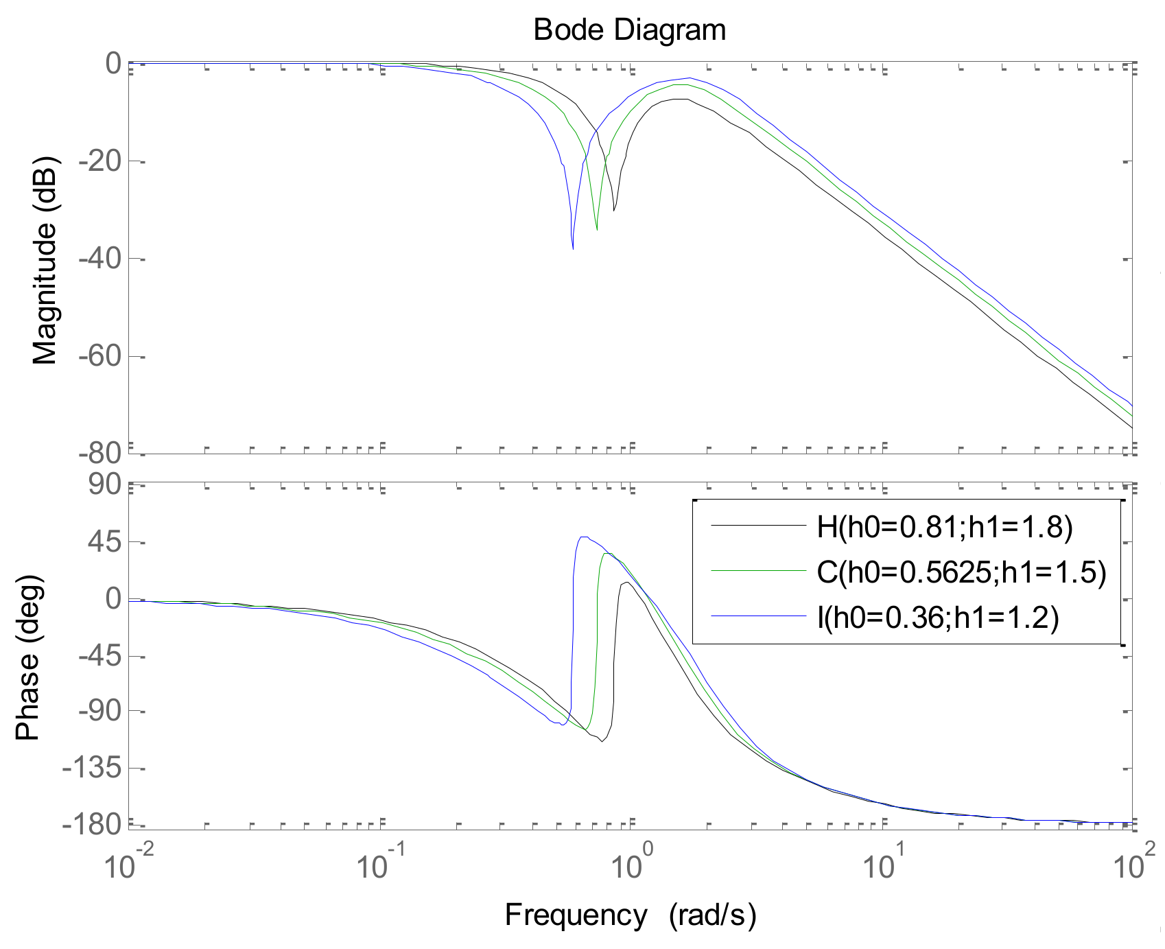
and
are coefficients of the desired dynamic equation. They are chosen based on the requirements of control system, such as settling time, overshooting, and so on. Because the desired dynamic equation is a second-order system,
and
can be calculated according to the second-order system, as follows:
where
is the desired settling time;
is the damping of desired dynamic system; and
is the natural frequency of desired dynamic system.
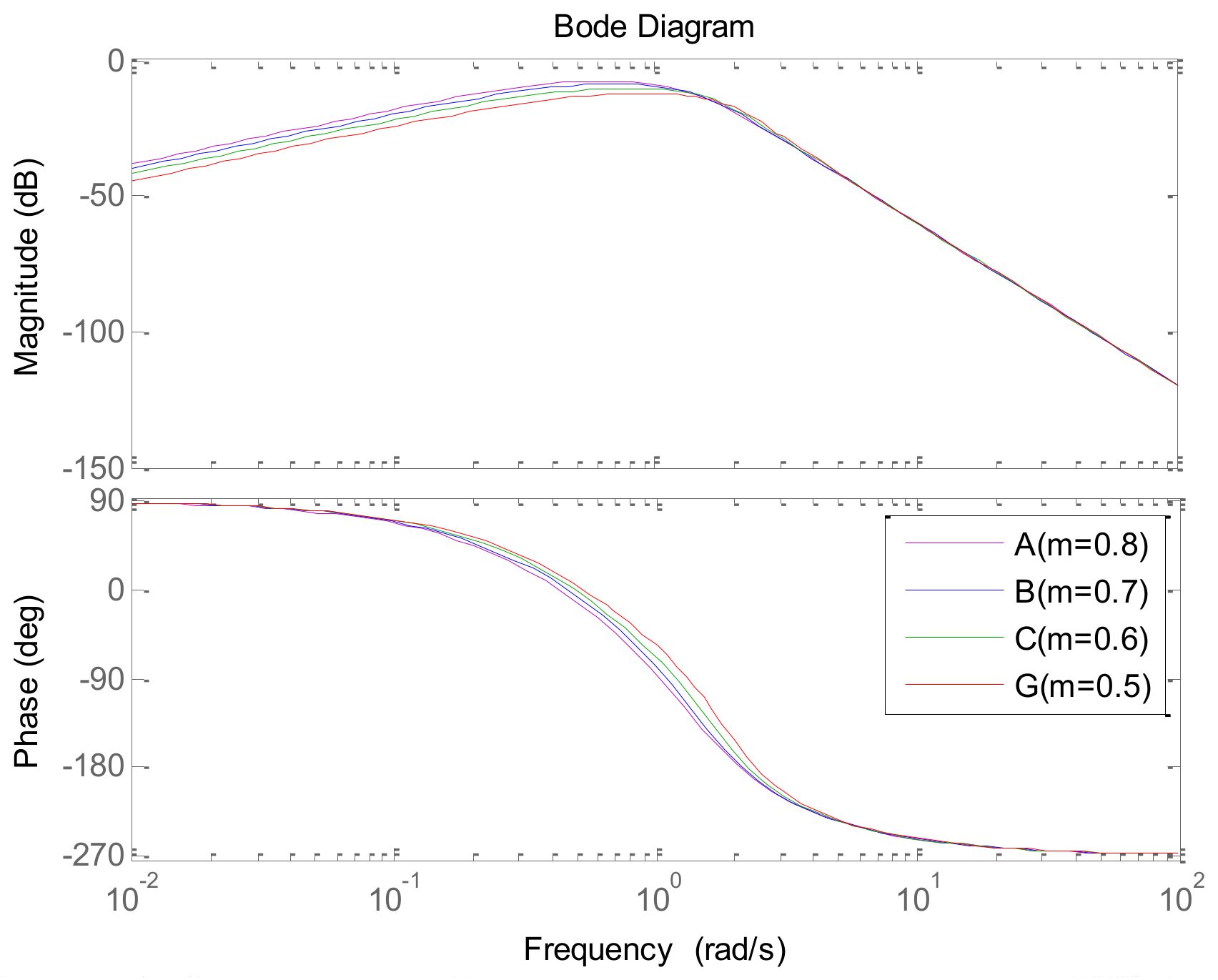
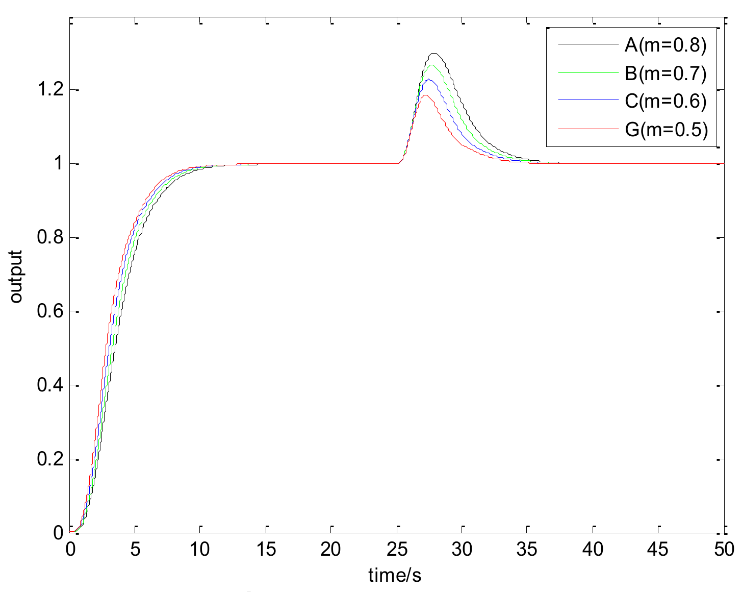
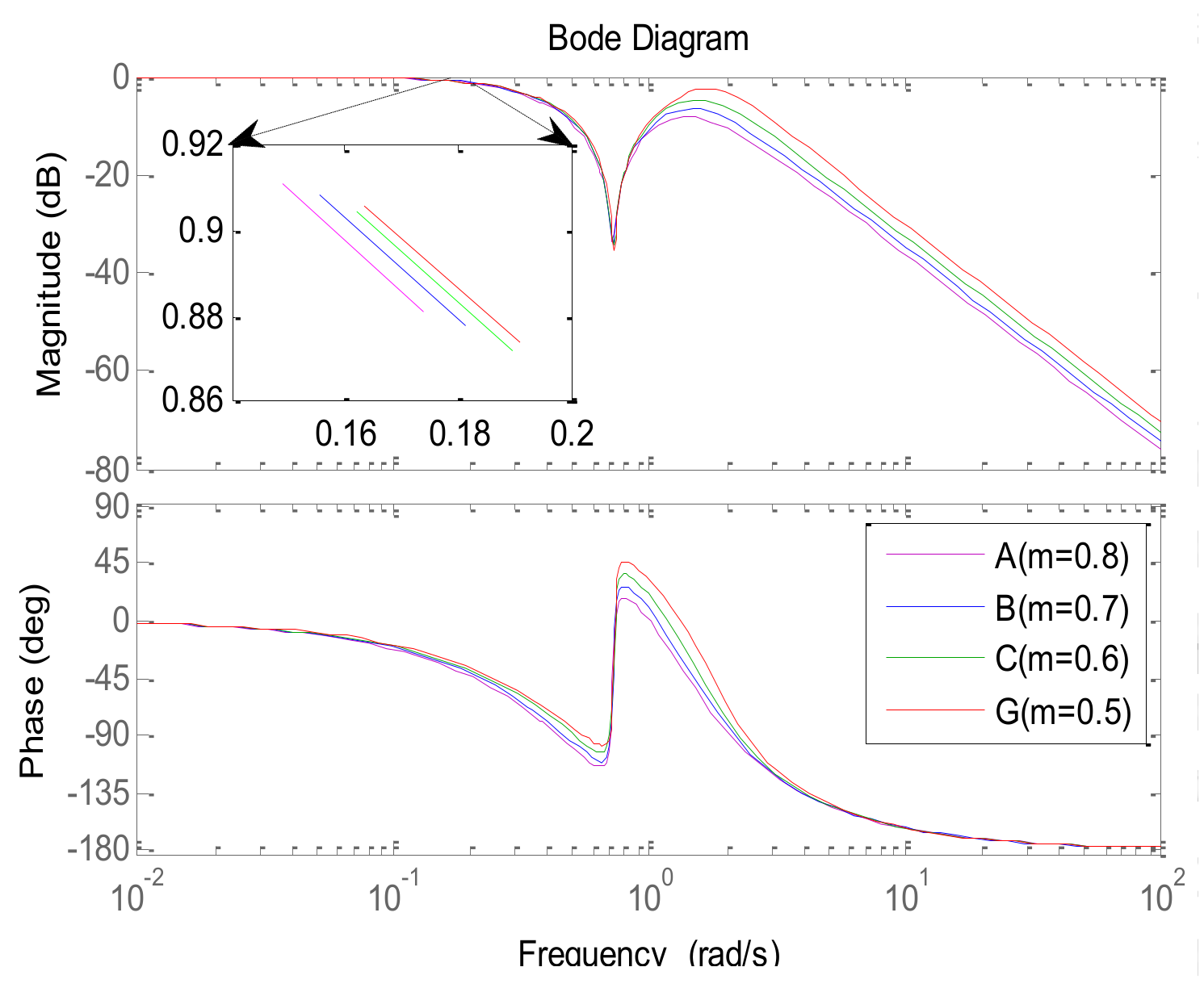
In order to make the overshooting as small as possible and make the settling time as short as possible,
is chosen. Considering the error between the actual dynamic and the desired dynamic, Equation (15) becomes
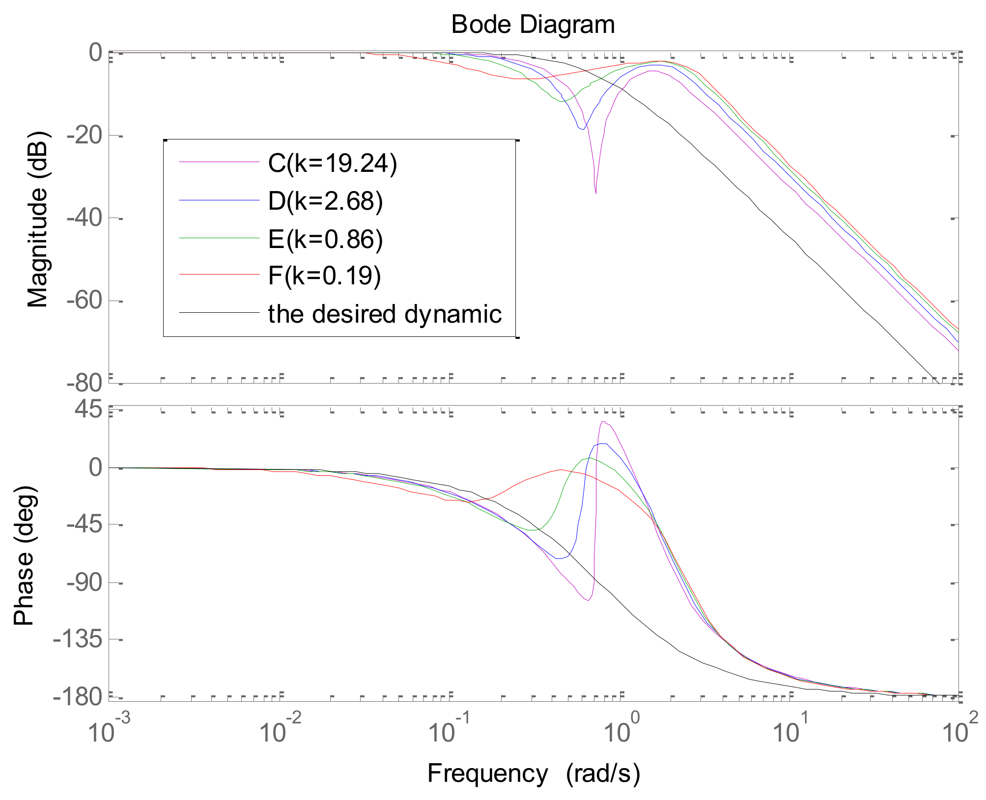
The stability margin increases with the increasing of the attenuation index
. It is well-known that there is a trade-off between performance and robustness [
26,
27]. Therefore, choosing an appropriate
is important to avoid the conflict with both
and
. According to our experience, the reasonable selecting region of
is generally
. One other thing to note is that a greater
is needed when the model is imprecise.
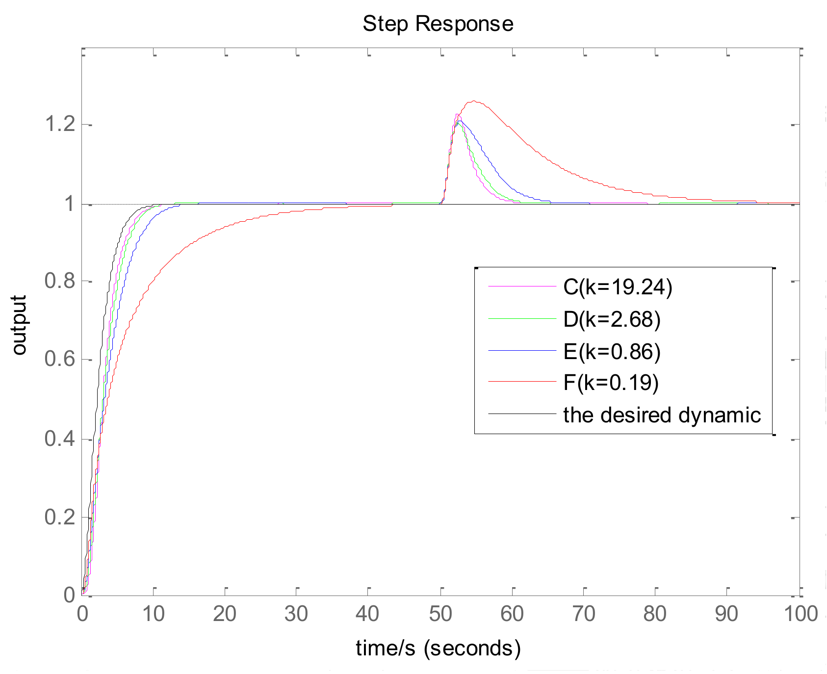
Combine Equation (2) with Equation (5) and do a Laplace transform, and the following equation is obtained:
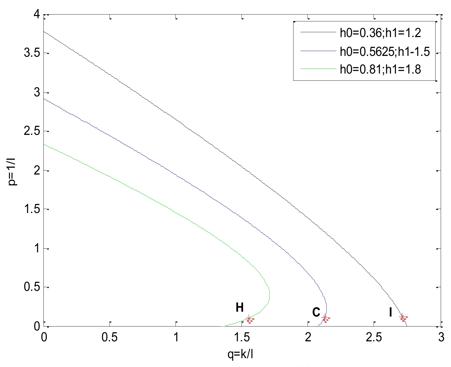
As shown in Equation (17), the response rate of the disturbance observer speeds up with increasing. So, the work point should be chosen nearby the q-axis in order to make as large as possible because in the plane.
The work point is chosen as follows.
First, substitute
into Equation (14), and the following equation is obtained.
Solve Equation (18), and and can be obtained.
Then, define
and substitute
into Equation (14), so
and
can be obtained. The point
is the work point in the
plane.
Finally, substitute and into Equation (13), and the controller parameters are obtained.
The steps of setting the controller parameters are shown as follows:
- (1)
Obtain the system model and choose proper , and values according to the requirements of system;
- (2)
Solve Equation (18), and then get and ;
- (3)
Get from Equation (19), substitute into Equation (14), and then get and ;
- (4)
Substitute and into Equation (13) to calculate the controller parameters. If there are closed-loop poles outside of the sector area, decrease both and simultaneously or only , and then turn to step (2); otherwise, continue;
- (5)
Do the step response and calculate the settling time and overshooting. If the settling time is not met, then increase both and or decrease , and turn to step (2); if the overshooting is too great, then decrease both and or increase , and turn to step (2); otherwise, continue;
- (6)
End.


