The Bias Compensation Based Parameter and State Estimation for Observability Canonical State-Space Models with Colored Noise

Abstract

This paper develops a bias compensation-based parameter and state estimation algorithm for the observability canonical state-space system corrupted by colored noise. The state-space system is transformed into a linear regressive model by eliminating the state variables. Based on the determination of the noise variance and noise model, a bias correction term is added into the least squares estimate, and the system parameters and states are computed interactively. The proposed algorithm can generate the unbiased parameter estimate. Two illustrative examples are given to show the effectiveness of the proposed algorithm.

1. Introduction

Mathematical models play a great role in adaptive control, online prediction and signal modeling [1,2,3,4]. The system models of physical plants can be constructed from first principle, but this method cannot work well when the physical mechanism of the true plants is not very clear [5,6]. Thus, data-driven-based black-box or gray-box state-space modeling can be used to approximate the law of motion [7,8,9]. The advantages of state-space modeling lie in that the model maps the relationship from inputs to outputs, and the states reflect the internal dynamic behavior of the plants. The estimation of state-space models may include both the unknown system parameters and the unmeasurable states [10,11]. It is well known that the Kalman filtering method captures the optimal state estimator based on the measurement data [12,13,14]. However, the model parameters of the system are generally assumed to be known in advance, and the statistical characteristics of measurement noise and process noise have to be chosen, which are hard to satisfy in practice [15,16,17].

On the identification of state-space models, the classical identification methods are the prediction-error methods, which require adequate knowledge of the system structures and parameters [18,19], and the subspace identification methods, which ignore the consistency of system parameter estimates [20,21,22]. Since the system states and parameters are involved in the state-space model, the simultaneous estimation of them is a feasible choice [23,24]. In this aspect, Pavelková and Kárný investigated the state and parameter estimation problem of the state-space model with bounded noise, providing a maximum estimator based on Bayesian theory [25]. By transforming the single-input multiple-output Hammerstein state-space model into the multivariable one, Ma et al. used the Kalman smoother to estimate the system states and the expectation maximization algorithm to compute parameter estimates [26]. Li et al. presented a maximum likelihood-based identification algorithm for the Wiener nonlinear system with a linear state-space subsystem [27]. Wang and Liu applied the recursive least squares algorithm to non-uniformly sampled state-space systems with the states being available and combined the singular value decomposition with the hierarchical identification principle for the identification of the system with the states being unavailable [28]. These studies were mainly focused on the state-space system with white noise.

In industrial processes, the observation data are often corrupted by colored noises [29,30,31]. As we have known, the parameter estimates generated by the recursive least squares algorithm for the system with colored noise are biased. To obtain the unbiased estimates, the bias compensation method was proposed [32]. The basic idea is to compensate the biased least squares estimate by adding a correction term [33,34,35]. Zhang investigated the parameter estimation of the multiple-input single-output linear system with colored noise and introduced a stable prefilter to preprocess the input data for the purpose of obtaining the unbiased estimate [36]. Zheng extended the bias compensation method to the errors-in-variables output-error system, where the input was contaminated by white noise and the output errors were modeled by colored noise [37]. On the identification of state-space models with colored noise, Wang et al. applied the Kalman filter algorithm to estimate the system states and developed a filtering-based recursive least squares algorithm for observer canonical state-space systems with colored noise [38]. On the basis of the work in [38], this paper discusses the state and parameter identification of the state-space model with colored noise and presents a bias compensation-based identification algorithm for jointly estimating the system parameters and states based on the bias compensation. The main contributions of the paper are as follows.

• By using the bias compensation, this paper derives the identification model and achieves the unbiased parameter estimation for observability canonical state-space models with colored noise.
• By employing the interactive identification, this paper explores the relationship between the noise parameters and variance and the bias correction term and realizes the simultaneous estimation of the system parameters, noise parameters and system states.

The rest of this paper is organized as follows. Section 2 demonstrates the problem formulation about the observability canonical state-space system and derives the identification model. Section 3 develops a bias compensation-based parameter and state estimation algorithm. Section 4 provides two illustrative examples to show that the proposed algorithm is effective. Finally, Section 5 offers some concluding remarks.

2. Problem Description and Identification Model

For narrative convenience, let us introduce some notation. The nomenclature is displayed in Table 1.

Table 1. The nomenclature for symbols.

Nomenclature
$\mathrm{T}$	matrix/vector transpose	${\mathit{A}}^{-1}$	inverse of the matrix A
$\mathrm{E}$	expectation operator	z	unit forward shift operator
$\parallel \mathit{X}\parallel$	2-norm of a matrix X	${\mathit{I}}_m$	$m\times m$ identity matrix
${\mathbf{1}}_n$	n-dimensional column vector whose elements are 1
$\widehat{\mathit{\theta }}\left(k\right)$	estimate of the parameter vector $\mathit{\theta }$ at instant k
$\mathit{\theta }(1:m)$	a vector consisting of the first entry to the m-th entry of $\mathit{\theta }$

Consider the following state-space system with colored noise,

$$\begin{array}{ccc}\hfill \mathit{x}(k+1)& =& \mathit{G}\mathit{x}\left(k\right)+\mathit{h}u\left(k\right),\hfill \end{array}$$

(1)

$$\begin{array}{ccc}\hfill y\left(k\right)& =& \mathit{f}\mathit{x}\left(k\right)+e\left(k\right),\hfill \end{array}$$

(2)

where $\mathit{x}\left(k\right):={[x_1\left(k\right),x_2\left(k\right),\cdots ,x_n\left(k\right)]}^{\mathrm{T}}\in {\mathbb{R}}^n$ is the state vector, $u\left(k\right)\in \mathbb{R}$ is the system input, $y\left(k\right)\in \mathbb{R}$ is the system output, $e\left(k\right)\in \mathbb{R}$ is a random noise and $\mathit{G}\in {\mathbb{R}}^{n\times n}$, $\mathit{h}\in {\mathbb{R}}^n$ and $\mathit{f}\in {\mathbb{R}}^{1\times n}$ are the system parameter matrix and vectors, defined as:

$$\begin{array}{ccc}\hfill \mathit{G}& :=& \left[\begin{array}{ccccc}0& 1& 0& \cdots & 0\\ 0& 0& 1& \ddots & ⋮\\ ⋮& ⋮& \ddots & \ddots & 0\\ 0& 0& \cdots & 0& 1\\ g_1& g_2& g_3& \cdots & g_n\end{array}\right]\in {\mathbb{R}}^{n\times n},\mathit{h}:=\left[\begin{array}{c}{h}_1\hfill \\ h_2\hfill \\ ⋮\hfill \\ h_{n-1}\hfill \\ h_n\hfill \end{array}\right]\in {\mathbb{R}}^n,\hfill \\ \hfill \mathit{f}& :=& [1,0,\cdots ,0,0]\in {\mathbb{R}}^{1\times n}.\hfill \end{array}$$

The external disturbance $e\left(k\right)$ can be fitted by a moving average process, an autoregressive process or an autoregressive moving average process. Without loss of generality, we consider $e\left(k\right)$ as a moving average noise process:

$$\begin{array}{ccc}\hfill e\left(k\right)& :=& (1+e_1{z}^{-1}+e_2{z}^{-2}+\cdots +e_{n_e}{z}^{-n_e})v\left(k\right),\hfill \end{array}$$

(3)

where $v\left(k\right)$ is the white noise with zero mean and variance $\delta$. Assume that $y\left(k\right)=0$, $u\left(k\right)=0$ and $v\left(k\right)=0$ for $k⩽0$. The objective is to estimate the parameters $g_i$, $h_i$ and $e_i$ and the system state $x\left(k\right)$ from the available input-output data $\left\{u\right(k),y(k):k=0,1,2,\cdots \}$.

Note that the system in Equations (1) and (2) is an observability canonical form, and the observability matrix T is an identity matrix, i.e.,

$$\mathit{T}={[{\mathit{f}}^{\mathrm{T}},{\left(\mathit{f}\mathit{G}\right)}^{\mathrm{T}},\cdots ,{\left(\mathit{f}{\mathit{G}}^{n-1}\right)}^{\mathrm{T}}]}^{\mathrm{T}}={\mathit{I}}_n.$$

(4)

From Equations (1) and (2), we have:

$$\begin{array}{ccc}\hfill y\left(k\right)& =& \mathit{f}\mathit{x}\left(k\right)+e\left(k\right),\hfill \\ \hfill y(k+1)& =& \mathit{f}\mathit{x}(k+1)+e(k+1)\hfill \end{array}$$

(5)

$$\begin{array}{ccc}& =& \mathit{f}\mathit{G}\mathit{x}\left(k\right)+\mathit{f}\mathit{h}u\left(k\right)+e(k+1),\hfill \\ \hfill y(k+2)& =& \mathit{f}\mathit{G}\mathit{x}(k+1)+\mathit{f}\mathit{h}u(k+1)+e(k+2)\hfill \end{array}$$

(6)

$$\begin{array}{ccc}& =& \mathit{f}{\mathit{G}}^2\mathit{x}\left(k\right)+\mathit{f}\mathit{G}\mathit{h}u\left(k\right)+\mathit{f}\mathit{h}u(k+1)+e(k+2),\hfill \\ & ⋮& \hfill \\ \hfill y(k+n-1)& =& \mathit{f}{\mathit{G}}^{n-1}\mathit{x}\left(k\right)+\mathit{f}{\mathit{G}}^{n-2}hu\left(k\right)+\mathit{f}{\mathit{G}}^{n-3}\mathit{h}u(k+1)+\cdots \hfill \end{array}$$

(7)

$$\begin{array}{ccc}& & +\mathit{f}\mathit{h}u(k+n-2)+e(k+n-1),\hfill \\ \hfill y(k+n)& =& \mathit{f}{\mathit{G}}^n\mathit{x}\left(k\right)+\mathit{f}{\mathit{G}}^{n-1}\mathit{h}u\left(k\right)+\mathit{f}{\mathit{G}}^{n-2}\mathit{h}u(k+1)+\cdots \hfill \end{array}$$

(8)

$$\begin{array}{ccc}& & +\mathit{f}\mathit{h}u(k+n-1)+e(k+n).\hfill \end{array}$$

(9)

Define the parameter matrix M and the information vectors ${\mathit{\varphi }}_{\mathrm{y}}\left(k\right)$, ${\mathit{\varphi }}_{\mathrm{u}}\left(k\right)$ and ${\mathit{\varphi }}_{\mathrm{e}}\left(k\right)$ as:

$$\begin{array}{ccc}\hfill \mathit{M}& :=& \left[\begin{array}{ccccc}0& 0& \cdots & 0& 0\\ \mathit{f}\mathit{h}& 0& \cdots & 0& 0\\ \mathit{f}\mathit{G}\mathit{h}& \mathit{f}\mathit{h}& \ddots & ⋮& ⋮\\ ⋮& ⋮& \ddots & 0& 0\\ \mathit{f}{\mathit{G}}^{n-2}\mathit{h}& \mathit{f}{\mathit{G}}^{n-3}\mathit{h}& \cdots & \mathit{f}\mathit{h}& 0\end{array}\right]\in {\mathbb{R}}^{n\times n},\hfill \\ \hfill {\mathit{\varphi }}_{\mathrm{y}}\left(k\right)& :=& {[y(k-n),y(k-n+1),\cdots ,y(k-1)]}^{\mathrm{T}}\in {\mathbb{R}}^n,\hfill \\ \hfill {\mathit{\varphi }}_{\mathrm{u}}\left(k\right)& :=& {[u(k-n),u(k-n+1),\cdots ,u(k-1)]}^{\mathrm{T}}\in {\mathbb{R}}^n,\hfill \\ \hfill {\mathit{\varphi }}_{\mathrm{e}}\left(k\right)& :=& {[e(k-n),e(k-n+1),\cdots ,e(k-1)]}^{\mathrm{T}}\in {\mathbb{R}}^n.\hfill \end{array}$$

According to Equations (5)–(8), we have:

$$\begin{array}{ccc}\hfill {\mathit{\varphi }}_{\mathrm{y}}(k+n)& =& \mathit{T}\mathit{x}\left(k\right)+\mathit{M}{\mathit{\varphi }}_{\mathrm{u}}(k+n)+{\mathit{\varphi }}_{\mathrm{e}}(k+n)\hfill \\ & =& \mathit{x}\left(k\right)+\mathit{M}{\mathit{\varphi }}_{\mathrm{u}}(k+n)+{\mathit{\varphi }}_{\mathrm{e}}(k+n).\hfill \end{array}$$

(10)

Equation (10) can be rewritten as:

$$\mathit{x}\left(k\right)={\mathit{\varphi }}_{\mathrm{y}}(k+n)-\mathit{M}{\mathit{\varphi }}_{\mathrm{u}}(k+n)-{\mathit{\varphi }}_{\mathrm{e}}(k+n).$$

(11)

Define the parameter vectors $\mathit{\vartheta }$, ${\mathit{\vartheta }}_{\mathrm{g}}$ and ${\mathit{\vartheta }}_{\mathrm{h}}$ and the information vectors ${\mathit{\varphi }}_{\mathrm{s}}\left(k\right)$ and ${\mathit{\varphi }}_{\mathrm{n}}\left(k\right)$ as:

$$\begin{array}{ccc}\hfill \mathit{\vartheta }& :=& {[{\mathit{\vartheta }}_{\mathrm{g}}^{\mathrm{T}},{\mathit{\vartheta }}_{\mathrm{h}}^{\mathrm{T}}]}^{\mathrm{T}}\in {\mathbb{R}}^{2n},\hfill \\ \hfill {\mathit{\vartheta }}_{\mathrm{g}}& :=& {\left[\mathit{f}{\mathit{G}}^n\right]}^{\mathrm{T}}\in {\mathbb{R}}^n,\hfill \\ \hfill {\mathit{\vartheta }}_{\mathrm{h}}& :=& {[-\mathit{f}{\mathit{G}}^{n}M+[\mathit{f}{\mathit{G}}^{n-1}\mathit{h},\mathit{f}{\mathit{G}}^{n-2}\mathit{h},\cdots ,\mathit{f}\mathit{h}]]}^{\mathrm{T}}\in {\mathbb{R}}^n,\hfill \\ \hfill {\mathit{\varphi }}_{\mathrm{s}}\left(k\right)& :=& \left[\begin{array}{c}{\mathit{\varphi }}_{\mathrm{y}}\left(k\right)\\ {\mathit{\varphi }}_{\mathrm{u}}\left(k\right)\end{array}\right]\in {\mathbb{R}}^{2n},{\mathit{\varphi }}_{\mathrm{n}}\left(k\right):=\left[\begin{array}{c}-{\mathit{\varphi }}_{\mathrm{e}}\left(k\right)\\ \mathbf{0}\end{array}\right]\in {\mathbb{R}}^{2n}.\hfill \end{array}$$

Inserting (11) into (9) yields:

$$\begin{array}{ccc}\hfill y(k+n)& =& \mathit{f}{\mathit{G}}^n[{\mathit{\varphi }}_{\mathrm{y}}(k+n)-\mathit{M}{\mathit{\varphi }}_{\mathrm{u}}(k+n)-{\mathit{\varphi }}_{\mathrm{e}}(k+n)]\hfill \\ & & +[\mathit{f}{\mathit{G}}^{n-1}\mathit{h},\mathit{f}{\mathit{G}}^{n-2}\mathit{h},\cdots ,\mathit{f}\mathit{h}]{\mathit{\varphi }}_{\mathrm{u}}(k+n)+e(k+n)\hfill \\ & =& {\mathit{\varphi }}_{\mathrm{y}}^{\mathrm{T}}(k+n){\mathit{\vartheta }}_{\mathrm{g}}+{\mathit{\varphi }}_{\mathrm{u}}^{\mathrm{T}}(k+n){\mathit{\vartheta }}_{\mathrm{h}}-{\mathit{\varphi }}_{\mathrm{e}}^{\mathrm{T}}(k+n){\mathit{\vartheta }}_{\mathrm{g}}+e(k+n)\hfill \\ & =& {\mathit{\varphi }}_{\mathrm{s}}^{\mathrm{T}}(k+n)\mathit{\vartheta }+{\mathit{\varphi }}_{\mathrm{n}}^{\mathrm{T}}(k+n)\mathit{\vartheta }+e(k+n).\hfill \end{array}$$

(12)

Define the intermediate variable:

$$w\left(k\right):={\mathit{\varphi }}_{\mathrm{n}}^{\mathrm{T}}\left(k\right)\mathit{\vartheta }+e\left(k\right).$$

(13)

Replacing $k+n$ in Equation (12) with k gives:

$$\begin{array}{ccc}\hfill y\left(k\right)& =& {\mathit{\varphi }}_{\mathrm{s}}^{\mathrm{T}}\left(k\right)\mathit{\vartheta }+{\mathit{\varphi }}_{\mathrm{n}}^{\mathrm{T}}\left(k\right)\mathit{\vartheta }+e\left(k\right)\hfill \end{array}$$

(14)

$$\begin{array}{ccc}\hfill & =& {\mathit{\varphi }}_{\mathrm{s}}^{\mathrm{T}}\left(k\right)\mathit{\vartheta }+w\left(k\right).\hfill \end{array}$$

(15)

Equation (14) or (15) is the system identification model of the state-space system in Equation (1), where the information vector ${\mathit{\varphi }}_{\mathrm{s}}\left(k\right)$ is composed of the observed data. Define the parameter vector ${\mathit{\vartheta }}_{\mathrm{v}}$ and the information vector ${\mathit{\varphi }}_{\mathrm{v}}\left(k\right)$ as:

$$\begin{array}{ccc}\hfill {\mathit{\vartheta }}_{\mathrm{v}}& :=& [e_1,e_2,\cdots ,e_{n_e}]\in {\mathbb{R}}^{n_e},\hfill \\ \hfill {\mathit{\varphi }}_{\mathrm{v}}\left(k\right)& :=& {[v(k-1),v(k-2),\cdots ,v(k-n_e)]}^{\mathrm{T}}\in {\mathbb{R}}^{n_e}.\hfill \end{array}$$

From Equation (3), we have:

$$e\left(k\right)={\mathit{\varphi }}_{\mathrm{v}}^{\mathrm{T}}\left(k\right){\mathit{\vartheta }}_{\mathrm{v}}+v\left(k\right).$$

(16)

Thus, we obtain the noise identification model in Equation (16). The following derives the bias compensation-based identification algorithm based on the system model in Equation (15) and the noise model in Equation (16).

3. The Bias Compensation-Based Parameter and State Estimation Algorithm

The algorithm includes two parts: the parameter estimation algorithm and the state estimation algorithm. Two parts are implemented in an interactive way.

3.1. The Parameter Estimation Algorithm

According to the identification model in Equation (15), define the cost function:

$$J\left(\mathit{\vartheta }\right):=\sum _{i=1}^k{[y\left(i\right)-{\mathit{\varphi }}_{\mathrm{s}}^{\mathrm{T}}\left(i\right)\mathit{\vartheta }]}^2$$

Using the least squares search and minimizing $J\left(\mathit{\vartheta }\right)$ give the least squares estimate ${\widehat{\mathit{\vartheta }}}_{\mathrm{LS}}\left(k\right)$ of the parameter vector $\mathit{\vartheta }$:

$$\begin{array}{ccc}\hfill {\widehat{\mathit{\vartheta }}}_{\mathrm{LS}}\left(k\right)& =& \mathit{P}\left(k\right)\sum _{i=1}^k{\mathit{\varphi }}_{\mathrm{s}}\left(i\right)y\left(i\right),\hfill \\ \hfill {\mathit{P}}^{-1}\left(k\right)& =& \sum _{i=1}^k{\mathit{\varphi }}_{\mathrm{s}}\left(i\right){\mathit{\varphi }}_{\mathrm{s}}^{\mathrm{T}}\left(i\right).\hfill \end{array}$$

(17)

Inserting (14) into (17) and using (13), we have:

$$\begin{array}{ccc}\hfill {\widehat{\mathit{\vartheta }}}_{\mathrm{LS}}\left(k\right)& =& \mathit{P}\left(k\right)\sum _{i=1}^k{\mathit{\varphi }}_{\mathrm{s}}\left(i\right)[{\mathit{\varphi }}_{\mathrm{s}}^{\mathrm{T}}\left(i\right)\mathit{\vartheta }+{\mathit{\varphi }}_{\mathrm{n}}^{\mathrm{T}}\left(i\right)\mathit{\vartheta }+e\left(i\right)]\hfill \\ & =& \mathit{\vartheta }+\mathit{P}\left(k\right)\sum _{i=1}^k{\mathit{\varphi }}_{\mathrm{s}}\left(i\right)[{\mathit{\varphi }}_{\mathrm{n}}^{\mathrm{T}}\left(i\right)\mathit{\vartheta }+e\left(i\right)].\hfill \end{array}$$

(18)

Obviously, the least squares estimate ${\widehat{\mathit{\vartheta }}}_{\mathrm{LS}}\left(k\right)$ in Equation (18) is a biased estimate since $e\left(k\right)$ is correlated noise. Equation (18) can be rewritten as:

$${\mathit{P}}^{-1}\left(k\right)[{\widehat{\mathit{\vartheta }}}_{\mathrm{LS}}\left(k\right)-\mathit{\vartheta }]=\sum _{i=1}^k{\mathit{\varphi }}_{\mathrm{s}}\left(i\right)[{\mathit{\varphi }}_{\mathrm{n}}^{\mathrm{T}}\left(i\right)\mathit{\vartheta }+e\left(i\right)].$$

Dividing by k and taking limits on both sides give:

$$\underset{k\to \infty }{lim}\frac{1}{k}\left[{\mathit{P}}^{-1}\left(k\right)({\widehat{\mathit{\vartheta }}}_{\mathrm{LS}}\left(k\right)-\mathit{\vartheta })\right]=\left[\underset{k\to \infty }{lim}\frac{1}{k}\sum _{i=1}^k{\mathit{\varphi }}_{\mathrm{s}}\left(i\right){\mathit{\varphi }}_{\mathrm{n}}^{\mathrm{T}}\left(i\right)\right]\mathit{\vartheta }+\underset{k\to \infty }{lim}\frac{1}{k}\sum _{i=1}^k{\mathit{\varphi }}_{\mathrm{s}}\left(i\right)e\left(i\right).$$

(19)

Note that $e\left(k\right)$ in Equation (19) is the moving average noise, and $v\left(k\right)$ is white noise with zero mean and variance $\delta$ and is independent of the inputs. From Equation (3), we have:

$$\begin{array}{ccc}\hfill R\left(0\right)& :=& \mathrm{E}\left[e^2\left(k\right)\right]=(1+e_1^2+e_2^2+\cdots +e_{n_e}^2)\delta =[1+{\mathit{\vartheta }}_{\mathrm{v}}^{\mathrm{T}}{\mathit{\vartheta }}_{\mathrm{v}}]\delta ,\hfill \\ \hfill R\left(i\right)& :=& \mathrm{E}\left[e(k-i)e\left(k\right)\right]=(e_i+e_{i+1}{e}_1+\cdots +e_{n_e}{e}_{n_e-i})\delta \hfill \\ & =& {\mathit{\vartheta }}_{\mathrm{v}}^{\mathrm{T}}(i:n_e)\left[\begin{array}{c}1\\ {\mathit{\vartheta }}_{\mathrm{v}}(1:n_e-i)\end{array}\right]\delta ,i=1,2,\cdots ,n_e,\hfill \end{array}$$

where $R\left(i\right)$ is the autocorrelation function of the noise $e\left(k\right)$ and $R\left(i\right)=0$ when $i>n_e$. Define the autocorrelation function vectors r and $\mathit{\zeta }$ and the autocorrelation function matrices R, $\mathsf{\Lambda }$ and Q as:

$$\begin{array}{ccc}\hfill \mathit{r}& :=& {[R\left(n\right),R(n-1),\cdots ,R\left(1\right),0,0\cdots ,0]}^{\mathrm{T}}\in {\mathbb{R}}^{2n},\hfill \end{array}$$

(20)

$$\begin{array}{ccc}\hfill \mathit{\zeta }& :=& {[R\left(n\right)/\delta ,R(n-1)/\delta ,\cdots ,R\left(1\right)/\delta ,0,0\cdots ,0]}^{\mathrm{T}}\in {\mathbb{R}}^{2n},\hfill \end{array}$$

(21)

$$\begin{array}{ccc}\hfill \mathit{R}& :=& \mathrm{diag}[\mathsf{\Lambda },\mathbf{0}]\in {\mathbb{R}}^{\left(2n\right)\times \left(2n\right)},\hfill \end{array}$$

(22)

$$\begin{array}{ccc}\hfill \mathsf{\Lambda }& :=& \left[\begin{array}{cccc}R\left(0\right)& R\left(1\right)& \cdots & R(n-1)\\ R\left(1\right)& R\left(0\right)& \cdots & R(n-2)\\ ⋮& ⋮& \ddots & ⋮\\ R(n-1)& R(n-2)& \cdots & R\left(0\right)\end{array}\right]\in {\mathbb{R}}^{n\times n},\hfill \end{array}$$

(23)

$$\begin{array}{ccc}\hfill \mathit{Q}& :=& \mathit{R}/\delta .\hfill \end{array}$$

(24)

In fact, $\mathsf{\Lambda }$ is a Toeplitz matrix consisting of n autocorrelation functions. Equation (19) can be rewritten as:

$$\underset{k\to \infty }{lim}\frac{1}{k}\left[{\mathit{P}}^{-1}\left(k\right)({\widehat{\mathit{\vartheta }}}_{\mathrm{LS}}\left(k\right)-\mathit{\vartheta })\right]=-(\mathit{R}\mathit{\vartheta }-\mathit{r}).$$

or:

$$\underset{k\to \infty }{lim}{\widehat{\mathit{\vartheta }}}_{\mathrm{LS}}\left(k\right)=\mathit{\vartheta }-k\mathit{P}\left(k\right)(\mathit{R}\mathit{\vartheta }-\mathit{r}).$$

(25)

It can be seen from Equation (25) that the bias of the least squares estimate ${\widehat{\mathit{\vartheta }}}_{\mathrm{LS}}\left(k\right)$ can be eliminated by adding a compensation term $\Delta \mathit{\vartheta }\left(k\right):=k\mathit{P}\left(k\right)(\mathit{R}\mathit{\vartheta }-\mathit{r})$. That is, the estimate ${\widehat{\mathit{\vartheta }}}_{\mathrm{C}}\left(k\right):={\widehat{\mathit{\vartheta }}}_{\mathrm{LS}}\left(k\right)+\Delta \mathit{\vartheta }\left(k\right)$ is an unbiased estimate of the true parameter vector $\mathit{\vartheta }$. Thus, the unbiased estimate ${\widehat{\mathit{\vartheta }}}_{\mathrm{C}}\left(k\right)$ can be computed by the following recursive expressions,

$$\begin{array}{ccc}\hfill {\widehat{\mathit{\vartheta }}}_{\mathrm{C}}\left(k\right)& =& {\widehat{\mathit{\vartheta }}}_{\mathrm{LS}}\left(k\right)+k\mathit{P}\left(k\right)[\widehat{\mathit{R}}\left(k\right){\widehat{\mathit{\vartheta }}}_{\mathrm{C}}\left(k\right)-\widehat{\mathit{r}}\left(k\right)]\hfill \\ & =& {\widehat{\mathit{\vartheta }}}_{\mathrm{LS}}\left(k\right)+k\widehat{\delta }\left(k\right)\mathit{P}\left(k\right)[\widehat{\mathit{Q}}\left(k\right){\widehat{\mathit{\vartheta }}}_{\mathrm{C}}\left(k\right)-\widehat{\mathit{\zeta }}\left(k\right)],\hfill \end{array}$$

(26)

$$\begin{array}{ccc}\hfill {\widehat{\mathit{\vartheta }}}_{\mathrm{LS}}\left(k\right)& =& {\widehat{\mathit{\vartheta }}}_{\mathrm{LS}}(k-1)+\mathit{P}\left(k\right){\mathit{\varphi }}_{\mathrm{s}}\left(k\right)[y\left(k\right)-{\mathit{\varphi }}_{\mathrm{s}}^{\mathrm{T}}\left(k\right){\widehat{\mathit{\vartheta }}}_{\mathrm{LS}}(k-1)],\hfill \end{array}$$

(27)

$$\begin{array}{ccc}\hfill {\mathit{P}}^{-1}\left(k\right)& =& {\mathit{P}}^{-1}(k-1)+{\parallel {\mathit{\varphi }}_{\mathrm{s}}\left(k\right)\parallel }^2,\mathit{P}\left(0\right)=p_0{\mathit{I}}_{2n},\hfill \end{array}$$

(28)

$$\begin{array}{ccc}\hfill {\mathit{\varphi }}_{\mathrm{s}}\left(k\right)& =& \left[\begin{array}{c}{\mathit{\varphi }}_{\mathrm{y}}\left(k\right)\\ {\mathit{\varphi }}_{\mathrm{u}}\left(k\right)\end{array}\right],{\widehat{\mathit{\vartheta }}}_{\mathrm{C}}\left(k\right)=\left[\begin{array}{c}{\widehat{\mathit{\vartheta }}}_{\mathrm{g}}\left(k\right)\\ {\widehat{\mathit{\vartheta }}}_{\mathrm{h}}\left(k\right)\end{array}\right].\hfill \end{array}$$

(29)

Equation (26) shows that the unbiased estimate ${\widehat{\mathit{\vartheta }}}_{\mathrm{C}}\left(k\right)$ is related to the estimates of R and r (i.e., the noise variance $\delta$ and the noise parameter vector ${\mathit{\vartheta }}_{\mathrm{v}}$). The following derives their estimates based on the interactive identification.

Let the least squares residual ${\epsilon }_{\mathrm{LS}}\left(i\right):=y\left(i\right)-{\mathit{\varphi }}_{\mathrm{s}}^{\mathrm{T}}\left(i\right){\widehat{\mathit{\vartheta }}}_{\mathrm{LS}}\left(k\right)$. Using Equation (14) and the relation ${\sum }_{i=1}^k{\epsilon }_{\mathrm{LS}}\left(i\right){\mathit{\varphi }}_{\mathrm{s}}^{\mathrm{T}}\left(i\right)=\mathbf{0}$ gives:

$$\begin{array}{ccc}\hfill \sum _{i=1}^k{\epsilon }_{\mathrm{LS}}^2\left(i\right)& =& \sum _{i=1}^k{\epsilon }_{\mathrm{LS}}\left(i\right)[{\mathit{\varphi }}_{\mathrm{s}}^{\mathrm{T}}\left(i\right)\mathit{\vartheta }+{\mathit{\varphi }}_{\mathrm{n}}^{\mathrm{T}}\left(i\right)\mathit{\vartheta }+e\left(i\right)-{\mathit{\varphi }}_{\mathrm{s}}^{\mathrm{T}}\left(i\right){\widehat{\mathit{\vartheta }}}_{\mathrm{LS}}\left(k\right)]\hfill \\ & =& \sum _{i=1}^k[{\mathit{\varphi }}_{\mathrm{s}}^{\mathrm{T}}\left(i\right)\mathit{\vartheta }+{\mathit{\varphi }}_{\mathrm{n}}^{\mathrm{T}}\left(i\right)\mathit{\vartheta }+e\left(i\right)-{\mathit{\varphi }}_{\mathrm{s}}^{\mathrm{T}}\left(i\right){\widehat{\mathit{\vartheta }}}_{\mathrm{LS}}\left(k\right)][{\mathit{\varphi }}_{\mathrm{n}}^{\mathrm{T}}\left(i\right)\mathit{\vartheta }+e\left(i\right)]\hfill \\ & =& \sum _{i=1}^k{\mathit{\varphi }}_{\mathrm{s}}^{\mathrm{T}}\left(i\right)[\mathit{\vartheta }-{\widehat{\mathit{\vartheta }}}_{\mathrm{LS}}\left(k\right)][{\mathit{\varphi }}_{\mathrm{n}}^{\mathrm{T}}\left(i\right)\mathit{\vartheta }+e\left(i\right)]+\sum _{i=1}^k{[{\mathit{\varphi }}_{\mathrm{n}}^{\mathrm{T}}\left(i\right)\mathit{\vartheta }+e\left(i\right)]}^2.\hfill \end{array}$$

Noting that R is a symmetric matrix, and using Equations (20)–(24), we have:

$$\begin{array}{ccc}\hfill \underset{k\to \infty }{lim}\frac{1}{k}\sum _{i=1}^k{\epsilon }_{\mathrm{LS}}^2\left(i\right)& =& -{\mathit{\vartheta }}^{\mathrm{T}}{\mathit{R}}^{\mathrm{T}}[\mathit{\vartheta }-{\widehat{\mathit{\vartheta }}}_{\mathrm{LS}}\left(k\right)]+{\mathit{r}}^{\mathrm{T}}[\mathit{\vartheta }-{\widehat{\mathit{\vartheta }}}_{\mathrm{LS}}\left(k\right)]+\mathit{\vartheta }\mathit{R}\mathit{\vartheta }-2{\mathit{r}}^{\mathrm{T}}\mathit{\vartheta }+R\left(0\right)\hfill \\ & =& {\mathit{\vartheta }}^{\mathrm{T}}\mathit{R}{\widehat{\mathit{\vartheta }}}_{\mathrm{LS}}\left(k\right)-{\mathit{r}}^{\mathrm{T}}[\mathit{\vartheta }+{\widehat{\mathit{\vartheta }}}_{\mathrm{LS}}\left(k\right)]+R\left(0\right)\hfill \\ & =& {\mathit{\vartheta }}^{\mathrm{T}}\delta \mathit{Q}{\widehat{\mathit{\vartheta }}}_{\mathrm{LS}}\left(k\right)-\delta {\mathit{\zeta }}^{\mathrm{T}}[\mathit{\vartheta }+{\widehat{\mathit{\vartheta }}}_{\mathrm{LS}}\left(k\right)]+\delta [1+{\mathit{\vartheta }}_{\mathrm{v}}^{\mathrm{T}}{\mathit{\vartheta }}_{\mathrm{v}}].\hfill \end{array}$$

Thus, we have:

$$\delta =\frac{{lim}_{k\to \infty }\frac{1}{k}{\sum }_{i=1}^k{\epsilon }_{\mathrm{LS}}^2\left(i\right)}{{\mathit{\vartheta }}^{\mathrm{T}}\mathit{Q}{\widehat{\mathit{\vartheta }}}_{\mathrm{LS}}\left(k\right)-{\mathit{\zeta }}^{\mathrm{T}}[\mathit{\vartheta }+{\widehat{\mathit{\vartheta }}}_{\mathrm{LS}}\left(k\right)]+1+{\mathit{\vartheta }}_{\mathrm{v}}^{\mathrm{T}}{\mathit{\vartheta }}_{\mathrm{v}}}.$$

Let $J\left(k\right):={\sum }_{i=1}^k{\epsilon }_{\mathrm{LS}}^2\left(i\right)$ be the cost function at time k, $\widehat{\mathit{Q}}\left(k\right)$ and $\widehat{\mathit{\zeta }}\left(k\right)$ be the estimates of Q and $\mathit{\zeta }$ at instant k, respectively. Then, the estimate of the noise variance $\delta$ can be computed by:

$$\begin{array}{cc}\hfill & \widehat{\delta }\left(k\right)=\frac{\frac{1}{k}J\left(k\right)}{{\widehat{\mathit{\vartheta }}}_{\mathrm{C}}^{\mathrm{T}}\left(k\right)\widehat{Q}\left(k\right){\widehat{\mathit{\vartheta }}}_{\mathrm{LS}}\left(k\right)-{\widehat{\mathit{\zeta }}}^{\mathrm{T}}\left(k\right)[{\widehat{\mathit{\vartheta }}}_{\mathrm{C}}\left(k\right)+{\widehat{\mathit{\vartheta }}}_{\mathrm{LS}}\left(k\right)]+1+{\widehat{\mathit{\vartheta }}}_{\mathrm{v}}^{\mathrm{T}}\left(k\right){\widehat{\mathit{\vartheta }}}_{\mathrm{v}}\left(k\right)},\hfill \end{array}$$

(30)

$$\begin{array}{cc}\hfill & J\left(k\right)=J(k-1)+\frac{{[y\left(k\right)-{\mathit{\varphi }}_{\mathrm{s}}^{\mathrm{T}}\left(k\right){\widehat{\mathit{\vartheta }}}_{\mathrm{LS}}(k-1)]}^2}{1+{\mathit{\varphi }}_{\mathrm{s}}^{\mathrm{T}}\left(k\right)P(k-1){\mathit{\varphi }}_{\mathrm{s}}\left(k\right)},\hfill \end{array}$$

(31)

$$\begin{array}{cc}\hfill & \widehat{\mathit{\zeta }}\left(k\right)={[\widehat{R}\left(n\right)/\widehat{\delta }(k-1),\widehat{R}(n-1)/\widehat{\delta }(k-1),\cdots ,\widehat{R}\left(1\right)/\widehat{\delta }(k-1),0,0\cdots ,0]}^{\mathrm{T}},\hfill \end{array}$$

(32)

$$\begin{array}{cc}\hfill & \widehat{Q}\left(k\right)=\left[\begin{array}{cc}\left[\begin{array}{cccc}1+{\widehat{\mathit{\vartheta }}}_{\mathrm{v}}^{\mathrm{T}}\left(k\right){\widehat{\mathit{\vartheta }}}_{\mathrm{v}}\left(k\right)& \widehat{R}\left(1\right)/\widehat{\delta }(k-1)& \cdots & \widehat{R}(n-1)/\widehat{\delta }(k-1)\\ \widehat{R}\left(1\right)/\widehat{\delta }(k-1)& 1+{\widehat{\mathit{\vartheta }}}_{\mathrm{v}}^{\mathrm{T}}\left(k\right){\widehat{\mathit{\vartheta }}}_{\mathrm{v}}\left(k\right)& \cdots & \widehat{R}(n-2)/\widehat{\delta }(k-1)\\ ⋮& ⋮& \ddots & ⋮\\ \widehat{R}(n-1)/\widehat{\delta }(k-1)& \widehat{R}(n-2)/\widehat{\delta }(k-1)& \cdots & 1+{\widehat{\mathit{\vartheta }}}_{\mathrm{v}}^{\mathrm{T}}\left(k\right){\widehat{\mathit{\vartheta }}}_{\mathrm{v}}\left(k\right)\end{array}\right]& \mathbf{0}\\ \mathbf{0}& \mathbf{0}\end{array}\right],\hfill \end{array}$$

(33)

$$\begin{array}{cc}\hfill & \frac{\widehat{R}\left(i\right)}{\widehat{\delta }(k-1)}={\widehat{\mathit{\vartheta }}}_{\mathrm{v}}^{\mathrm{T}}(i:n_e)\left[\begin{array}{c}1\\ {\widehat{\mathit{\vartheta }}}_{\mathrm{v}}(1:n_e-i)\end{array}\right],i=1,2,\cdots ,n_e.\hfill \end{array}$$

(34)

Note that Equations (30)–(34) involve the estimate ${\widehat{\mathit{\vartheta }}}_{\mathrm{v}}\left(k\right)$ of the noise parameter vector ${\mathit{\vartheta }}_{\mathrm{v}}$, which can be computed by the noise model in Equation (16). Let $\widehat{e}\left(k\right)$ and $\widehat{v}\left(k\right)$ be the estimates of $e\left(k\right)$ and $v\left(k\right)$, respectively. Define the noise information vectors:

$$\begin{array}{ccc}\hfill {\widehat{\mathit{\varphi }}}_{\mathrm{n}}\left(k\right)& :=& {[-\widehat{e}(k-n),-\widehat{e}(k-n+1),\cdots ,-\widehat{e}(k-1),0,0,\cdots ,0]}^{\mathrm{T}}\in {\mathbb{R}}^{2n},\hfill \end{array}$$

(35)

$$\begin{array}{ccc}\hfill {\widehat{\mathit{\varphi }}}_{\mathrm{v}}\left(k\right)& :=& {[\widehat{v}(k-1),\widehat{v}(k-2),\cdots ,\widehat{v}(k-n_e)]}^{\mathrm{T}}\in {\mathbb{R}}^{n_e}.\hfill \end{array}$$

(36)

From Equations (14) and (16), we have:

$$\begin{array}{ccc}\hfill \widehat{e}\left(k\right)& =& y\left(k\right)-{\mathit{\varphi }}_{\mathrm{s}}^{\mathrm{T}}\left(k\right){\widehat{\mathit{\vartheta }}}_{\mathrm{C}}\left(k\right)-{\widehat{\mathit{\varphi }}}_{\mathrm{n}}^{\mathrm{T}}\left(k\right){\widehat{\mathit{\vartheta }}}_{\mathrm{C}}\left(k\right),\hfill \end{array}$$

(37)

$$\begin{array}{ccc}\hfill \widehat{v}\left(k\right)& =& \widehat{e}\left(k\right)-{\widehat{\mathit{\varphi }}}_{\mathrm{v}}^{\mathrm{T}}\left(k\right){\widehat{\mathit{\vartheta }}}_{\mathrm{v}}\left(k\right).\hfill \end{array}$$

(38)

Using the least squares principle, the estimate ${\widehat{\mathit{\vartheta }}}_{\mathrm{v}}\left(k\right)$ of ${\mathit{\vartheta }}_{\mathrm{v}}$ in Equation (16) can be computed by:

$$\begin{array}{ccc}\hfill {\widehat{\mathit{\vartheta }}}_{\mathrm{v}}\left(k\right)& =& {\widehat{\mathit{\vartheta }}}_{\mathrm{v}}(k-1)+{\mathit{P}}_{\mathrm{v}}\left(k\right){\widehat{\mathit{\varphi }}}_{\mathrm{v}}\left(k\right)[\widehat{e}\left(k\right)-{\widehat{\mathit{\varphi }}}_{\mathrm{v}}^{\mathrm{T}}\left(k\right){\widehat{\mathit{\vartheta }}}_{\mathrm{v}}(k-1)],\hfill \end{array}$$

(39)

$$\begin{array}{ccc}\hfill {\mathit{P}}_{\mathrm{v}}^{-1}\left(k\right)& =& {\mathit{P}}_{\mathrm{v}}^{-1}(k-1)+{\widehat{\mathit{\varphi }}}_{\mathrm{v}}\left(k\right){\widehat{\mathit{\varphi }}}_{\mathrm{v}}^{\mathrm{T}}\left(k\right).\hfill \end{array}$$

(40)

Thus, Equations (26)–(40) form the bias compensation-based parameter estimation (BC-PE) algorithm for identifying the parameter vector $\mathit{\vartheta }$. The BC-PE algorithm is an interactive estimation process: we can compute the estimates ${\widehat{\mathit{\vartheta }}}_{\mathrm{v}}\left(k\right)$ and $\widehat{\delta }\left(k\right)$; with these obtained variable estimates, we derive the estimate of R and r and then update the unbiased estimate ${\widehat{\mathit{\vartheta }}}_{\mathrm{C}}\left(k\right)$ using Equations (26)–(29).

3.2. The State Estimation Algorithm

When the system parameter estimation and the noise estimation $\widehat{e}\left(k\right)$ are obtained from the BC-PE algorithm, we can estimate the system state $\mathit{x}\left(t\right)$ using Equation (11).

Post-multiplying Equation (4) by h and letting the elements of each row be equal, we have:

$$\mathit{f}{\mathit{G}}^{i-1}\mathit{h}=h_i,i=1,2,\cdots ,n.$$

Then, the parameter matrix M can be expressed as:

$$\mathit{M}=\left[\begin{array}{ccccc}0& 0& \cdots & 0& 0\\ h_1& 0& \cdots & 0& 0\\ h_2& h_1& \ddots & ⋮& ⋮\\ ⋮& ⋮& \ddots & 0& 0\\ h_{n-1}& h_{n-2}& \cdots & h_1& 0\end{array}\right].$$

Post-multiplying Equation (4) by G and letting the elements of n-th row be equal, we have:

$$\mathit{f}{\mathit{G}}^n=[g_1,g_2,\cdots ,g_n].$$

According to the definitions of ${\mathit{\vartheta }}_{\mathrm{g}}$ and ${\mathit{\vartheta }}_{\mathrm{h}}$, we have:

$$\begin{array}{ccc}\hfill {\mathit{\vartheta }}_{\mathrm{g}}& =& {\left[\mathit{f}{\mathit{G}}^n\right]}^{\mathrm{T}}={[g_1,g_2,\cdots ,g_n]}^{\mathrm{T}},\hfill \\ \hfill {\mathit{\vartheta }}_{\mathrm{h}}& =& {[-\mathit{f}{\mathit{G}}^n\mathit{M}+[\mathit{f}{\mathit{G}}^{n-1}\mathit{h},\mathit{f}{\mathit{G}}^{n-2}\mathit{h},\cdots ,\mathit{f}\mathit{h}]]}^{\mathrm{T}}\hfill \\ & =& \left[\begin{array}{c}-h_1{g}_2-h_2{g}_3-\cdots -h_{n-1}{g}_n+h_n\\ -h_1{g}_3-h_2{g}_4-\cdots -h_{n-2}{g}_n+h_{n-1}\\ ⋮\\ -h_1{g}_n+h_2\\ h_1\end{array}\right]=\left[\begin{array}{ccccc}-g_2& -g_3& \cdots & -g_n& 1\\ -g_3& -g_4& \cdots & 1& 0\\ ⋮& ⋮& ⋮& ⋮\\ -g_n& 1& \cdots & 0& 0\\ 1& 0& \cdots & 0& 0\end{array}\right]\left[\begin{array}{c}{h}_1\\ h_2\\ ⋮\\ h_{n-1}\\ h_n\end{array}\right].\hfill \end{array}$$

Once the estimate of the parameter vector $\mathit{\vartheta }$ is computed by the BC-PE algorithm in Equations (26)–(40), we can extract the estimates ${\widehat{\mathit{\vartheta }}}_{\mathrm{g}}\left(k\right)$ and ${\widehat{\mathit{\vartheta }}}_{\mathrm{h}}\left(k\right)$ of the parameter vectors ${\mathit{\vartheta }}_{\mathrm{g}}$ and ${\mathit{\vartheta }}_{\mathrm{h}}$. Then, the estimates ${\widehat{g}}_i\left(k\right)$ and ${\widehat{h}}_i\left(k\right)$ can be computed by:

$$\begin{array}{ccc}\hfill {\widehat{\mathit{\vartheta }}}_{\mathrm{g}}\left(k\right)& =& {[{\widehat{g}}_1\left(k\right),{\widehat{g}}_2\left(k\right),\cdots ,{\widehat{g}}_n\left(k\right)]}^{\mathrm{T}},\hfill \end{array}$$

(41)

$$\begin{array}{ccc}\hfill \left[\begin{array}{c}{\widehat{h}}_1\left(k\right)\\ {\widehat{h}}_2\left(k\right)\\ ⋮\\ {\widehat{h}}_{n-1}\left(k\right)\\ {\widehat{h}}_n\left(k\right)\end{array}\right]& =& {\left[\begin{array}{ccccc}-{\widehat{g}}_2\left(k\right)& -{\widehat{g}}_3\left(k\right)& \cdots & -{\widehat{g}}_n\left(k\right)& 1\\ -{\widehat{g}}_3\left(k\right)& -{\widehat{g}}_4\left(k\right)& \cdots & 1& 0\\ ⋮& ⋮& ⋮& ⋮\\ -{\widehat{g}}_n\left(k\right)& 1& \cdots & 0& 0\\ 1& 0& \cdots & 0& 0\end{array}\right]}^{-1}{\widehat{\mathit{\vartheta }}}_{\mathrm{h}}\left(k\right).\hfill \end{array}$$

(42)

From Equation (11), we have:

$$\mathit{x}(k-n)={\mathit{\varphi }}_{\mathrm{y}}\left(k\right)-\mathit{M}{\mathit{\varphi }}_{\mathrm{u}}\left(k\right)-{\mathit{\varphi }}_{\mathrm{e}}\left(k\right).$$

Replacing M and ${\mathit{\varphi }}_{\mathrm{e}}\left(k\right)$ with their corresponding estimates $\widehat{\mathit{M}}\left(k\right)$ and ${\widehat{\mathit{\varphi }}}_{\mathrm{e}}\left(k\right)$, we have:

$$\begin{array}{ccc}\hfill \widehat{\mathit{x}}(k-n)& =& {\mathit{\varphi }}_{\mathrm{y}}\left(k\right)-\widehat{\mathit{M}}\left(k\right){\mathit{\varphi }}_{\mathrm{u}}\left(k\right)-{\widehat{\mathit{\varphi }}}_{\mathrm{e}}\left(k\right),\hfill \end{array}$$

(43)

$$\begin{array}{ccc}\hfill {\mathit{\varphi }}_{\mathrm{y}}\left(k\right)& =& {[y(k-n),y(k-n+1),\cdots ,y(k-1)]}^{\mathrm{T}},\hfill \end{array}$$

(44)

$$\begin{array}{ccc}\hfill {\mathit{\varphi }}_{\mathrm{u}}\left(k\right)& =& {[u(k-n),u(k-n+1),\cdots ,u(k-1)]}^{\mathrm{T}},\hfill \end{array}$$

(45)

$$\begin{array}{ccc}\hfill {\widehat{\mathit{\varphi }}}_{\mathrm{e}}\left(k\right)& =& {[\widehat{e}(k-n),\widehat{e}(k-n+1),\cdots ,\widehat{e}(k-1)]}^{\mathrm{T}},\hfill \end{array}$$

(46)

$$\begin{array}{ccc}\hfill \widehat{\mathit{M}}\left(k\right)& =& \left[\begin{array}{ccccc}0& 0& \cdots & 0& 0\\ {\widehat{h}}_1\left(k\right)& 0& \cdots & 0& 0\\ {\widehat{h}}_2\left(k\right)& {\widehat{h}}_1\left(k\right)& \ddots & ⋮& ⋮\\ ⋮& ⋮& \ddots & 0& 0\\ {\widehat{h}}_{n-1}\left(k\right)& {\widehat{h}}_{n-2}\left(k\right)& \cdots & {\widehat{h}}_1\left(k\right)& 0\end{array}\right].\hfill \end{array}$$

(47)

Equations (41)–(47) form the state estimation algorithm for the state-space system in Equation (1). Let $\mathit{\theta }:={[{\mathit{g}}^{\mathrm{T}},{\mathit{h}}^{\mathrm{T}},{\mathit{\vartheta }}_{\mathrm{v}}^{\mathrm{T}}]}^{\mathrm{T}}\in {\mathbb{R}}^{2n+n_e}$, $\mathit{g}:=[g_1,g_2,\cdots ,g_n]\in {\mathbb{R}}^n$. By interactively implementing the parameter estimation algorithm in Equations (26)–(40) and the state estimation algorithm in Equations (41)–(47), the estimation of the system parameter vector $\mathit{\theta }$ and the state $\mathit{x}\left(k\right)$ can be obtained.

The steps for implementing the bias compensation-based parameter and state estimation (BC-PSE) algorithm in Equations (26) and (47) for state-space systems with colored noise are listed as follows.

• Let $k=1$, and set the initial values ${\widehat{\mathit{\vartheta }}}_{\mathrm{LS}}\left(0\right)={\widehat{\mathit{\vartheta }}}_{\mathrm{C}}\left(0\right)={\mathbf{1}}_{2n}/p_0$, ${\widehat{\mathit{\vartheta }}}_{\mathrm{v}}\left(0\right)={\mathbf{1}}_{n_e}/p_0$, $\mathit{P}\left(0\right)=p_0{I}_{2n}$, $J\left(0\right)=0$, $p_0={10}^6$.
• Collect the input-output data $u\left(k\right)$ and $y\left(k\right)$. Construct ${\mathit{\varphi }}_{\mathrm{y}}\left(k\right)$ using Equation (44), ${\mathit{\varphi }}_{\mathrm{u}}\left(k\right)$ using Equation (45) and ${\mathit{\varphi }}_{\mathrm{s}}\left(k\right)$ using Equation (29).
• Compute $\mathit{P}\left(k\right)$ using Equation (28) and $J\left(k\right)$ using Equation (31). Update the parameter estimate ${\widehat{\mathit{\vartheta }}}_{\mathrm{LS}}\left(k\right)$ using Equation (27).
• Construct ${\widehat{\mathit{\varphi }}}_{\mathrm{n}}\left(k\right)$ using Equation (35) and ${\widehat{\mathit{\varphi }}}_{\mathrm{v}}\left(k\right)$ using Equation (36). Compute $\widehat{e}\left(k\right)$ using Equation (37) and $\widehat{v}\left(k\right)$ using Equation (38), and compute ${\mathit{P}}_{\mathrm{v}}\left(k\right)$ using Equation (40). Update the noise parameter estimate ${\widehat{\mathit{\vartheta }}}_{\mathrm{v}}\left(k\right)$ using Equation (39).
• Compute $\widehat{\mathit{\zeta }}\left(k\right)$, $\widehat{\mathit{Q}}\left(k\right)$ and $\widehat{R}\left(i\right)/\widehat{\delta }(k-1)$ using Equations (32)–(34). Compute $\widehat{\delta }\left(k\right)$ using Equation (30) and ${\widehat{\mathit{\vartheta }}}_{\mathrm{C}}\left(k\right)$ using Equation (26).
• Read ${\widehat{\mathit{\vartheta }}}_{\mathrm{g}}\left(k\right)$ and ${\widehat{\mathit{\vartheta }}}_{\mathrm{h}}\left(k\right)$ using Equation (29). Acquire the parameter estimates ${\widehat{g}}_i\left(k\right)$ and ${\widehat{h}}_i\left(k\right)$ using Equations (41) and (42).
• Construct ${\widehat{\mathit{\varphi }}}_{\mathrm{e}}\left(k\right)$ using Equation (46) and $\widehat{\mathit{M}}\left(k\right)$ using Equation (47).
• Compute the state estimate $\widehat{\mathit{x}}\left(k\right)$ using Equation (43).
• Let $\widehat{\mathit{\theta }}\left(k\right):=\left[\begin{array}{c}\widehat{\mathit{g}}\left(k\right)\\ \widehat{\mathit{h}}\left(k\right)\\ {\widehat{\mathit{\vartheta }}}_{\mathrm{v}}\left(k\right)\end{array}\right]$. If $k<L$, increase k by one, and go to Step 2; otherwise, stop, and obtain the parameter estimation vector $\widehat{\mathit{\theta }}\left(L\right)$.

4. Examples

Example 1.

Consider the following state-space system with moving average noise,

$$\begin{array}{ccc}\hfill \mathit{x}(k+1)& =& \left[\begin{array}{cc}0& 1\\ g_1& g_2\end{array}\right]\mathit{x}\left(k\right)+\left[\begin{array}{c}{h}_1\\ h_2\end{array}\right]u\left(k\right)=\left[\begin{array}{cc}0& 1\\ -0.90& 0.80\end{array}\right]\mathit{x}\left(k\right)+\left[\begin{array}{c}1.10\\ -1.60\end{array}\right]u\left(k\right),\hfill \\ \hfill y\left(k\right)& =& [1,0]\mathit{x}\left(k\right)+e\left(k\right),\hfill \\ \hfill e\left(k\right)& =& (1+e_1{z}^{-1}+e_2{z}^{-2})v\left(k\right)=(1+0.20z^{-1}-0.60z^{-1})v\left(k\right).\hfill \end{array}$$

The parameter vector to be estimated is:

$$\begin{array}{ccc}\hfill \mathbf{\theta }& =& {[g_1,g_2,h_1,h_2,e_1,e_2]}^{\mathrm{T}}={[-0.90,0.80,1.10,-1.60,0.20,-0.60]}^{\mathrm{T}}.\hfill \end{array}$$

In simulation, the input $\left\{u\right(k\left)\right\}$ is set as a persistent excitation sequence and $\left\{v\right(k\left)\right\}$ as a zero-mean noise sequence with variance $\delta =0.25$. Take the data length $L=1200$. Use the first 1000 data and apply the BC-PSE algorithm to get the estimates of the parameter vector $\mathit{\theta }$ and the system state $\mathit{x}\left(k\right)$. The parameter estimates and their errors under different noise variances are displayed in Table 2 and Figure 1, where the estimation error $\tau :=\parallel \widehat{\mathit{\theta }}\left(k\right)-\mathit{\theta }\parallel /\parallel \mathit{\theta }\parallel \times 100\%$. The parameter estimate $\widehat{\mathit{\theta }}\left(k\right)$ versus k is plotted in Figure 2, and the state estimate $\widehat{\mathit{x}}\left(k\right)$ computed by the BC-PSE algorithm is illustrated in Figure 3 and Figure 4.

Table 2. The bias compensation-based parameter estimates and errors for Example 1.

$\mathit{\delta }$	k	${\mathit{g}}_1$	${\mathit{g}}_2$	${\mathit{h}}_1$	${\mathit{h}}_2$	${\mathit{e}}_1$	${\mathit{e}}_2$	$\mathit{\tau }(\%)$
$1.00$	20	−0.90672	0.58805	2.47895	−2.33308	0.12542	−1.41696	74.94801
	50	−0.91146	0.77864	1.56458	−1.45439	0.06347	−0.68669	21.66474
	100	−0.89769	0.78062	1.45065	−1.56252	0.11477	−0.61555	15.33989
	200	−0.89947	0.79122	1.18977	−1.58852	0.18174	−0.62250	4.02568
	500	−0.90289	0.79326	1.19050	−1.56703	0.17911	−0.62993	4.35605
	1000	−0.89502	0.79742	1.14729	−1.63721	0.18966	−0.61945	2.71347
$0.25$	20	−0.89902	0.68391	1.87036	−1.86695	0.37006	−0.70475	35.74537
	50	−0.90830	0.79067	1.34730	−1.49092	0.18690	−0.51892	11.92791
	100	−0.90003	0.79044	1.28652	−1.56142	0.20501	−0.50891	8.91773
	200	−0.90083	0.79596	1.15147	−1.58293	0.22360	−0.53086	3.84174
	500	−0.90199	0.79695	1.14809	−1.57856	0.20617	−0.56528	2.67739
	1000	−0.89776	0.79869	1.12493	−1.61634	0.20773	−0.57641	1.63983
True values		−0.90000	0.80000	1.10000	−1.60000	0.20000	−0.60000	0.00000

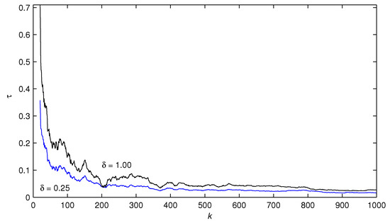
Figure 1. The estimation errors $\tau$ versus k with different noise variances for Example 1.

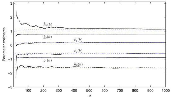
Figure 2. The parameter estimates $\widehat{\mathit{\theta }}\left(k\right)$ versus k for Example 1.

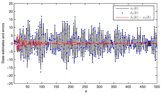
Figure 3. The state $x_1\left(k\right)$ and the estimated state ${\widehat{x}}_1\left(k\right)$ versus k for Example 1 ($\delta =0.25$).

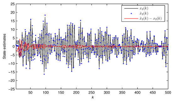
Figure 4. The state $x_2\left(k\right)$ and the estimated state ${\widehat{x}}_2\left(k\right)$ versus k for Example 1 ($\delta =0.25$).

The remaining 200 data from $k=1001$–1200 are taken to test the effectiveness of the estimated model. As a comparison, the curves of the estimated output $\widehat{y}\left(k\right)$ and the predicted output $y\left(k\right)$ are depicted in Figure 5.

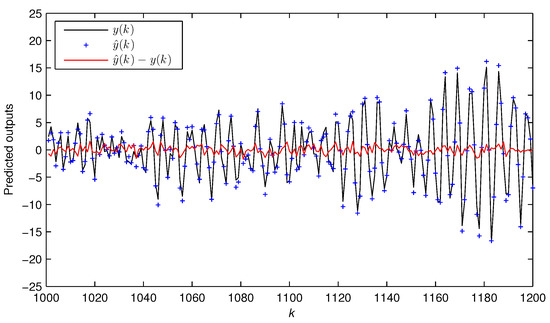
Figure 5. The actual output $y\left(k\right)$ and the estimated output $\widehat{y}\left(k\right)$ versus k for Example 1.

Example 2.

Consider a third-order observability canonical state-space system,

$$\begin{array}{ccc}\hfill \mathit{x}(k+1)& =& \left[\begin{array}{ccc}0& 1& 0\\ 0& 0& 1\\ -0.80& 0.50& 0.60\end{array}\right]\mathit{x}\left(k\right)+\left[\begin{array}{c}2.20\\ 0.30\\ 0.20\end{array}\right]u\left(k\right),\hfill \\ \hfill y\left(k\right)& =& [1,0,0]\mathit{x}\left(k\right)+e\left(k\right),\hfill \\ \hfill e\left(k\right)& =& (1+e_1{z}^{-1}+e_2{z}^{-2})v\left(k\right)=(1+0.50z^{-1}+0.40z^{-1})v\left(k\right).\hfill \end{array}$$

The parameter vector to be estimated is:

$$\begin{array}{ccc}\hfill \mathbf{\theta }& =& {[g_1,g_2,g_3,h_1,h_2,h_3,e_1,e_2]}^{\mathrm{T}}={[-0.80,0.50,0.60,2.20,0.30,0.20,0.50,0.40]}^{\mathrm{T}}.\hfill \end{array}$$

The simulation conditions are the same as those in Example 1. Table 3 and Figure 6 compare the bias compensation-based parameter estimates and errors under noise variances $\delta =0.25$ and $\delta =1.00$. Figure 7 and Figure 8 depict the curves of the parameter estimates $\widehat{\mathit{\theta }}\left(k\right)$ versus the instant k.

Table 3. The bias compensation-based parameter estimates and errors for Example 2.

$\mathit{\delta }$	k	${\mathit{g}}_1$	${\mathit{g}}_2$	${\mathit{g}}_3$	${\mathit{h}}_1$	${\mathit{h}}_2$	${\mathit{h}}_3$	${\mathit{e}}_1$	${\mathit{e}}_2$	$\mathit{\tau }(\%)$
$1.00$	20	−0.62874	0.23404	0.69918	2.71399	−0.51430	0.03521	0.55758	0.54550	40.52480
	50	−0.63162	0.17455	0.82387	2.36896	−0.10338	0.17046	0.57261	0.36257	24.04086
	100	−0.72920	0.37705	0.69853	2.10786	0.00205	0.03490	0.53153	0.47341	15.57075
	200	−0.77990	0.43541	0.64826	2.07686	0.11157	0.16642	0.52363	0.43391	9.54558
	500	−0.80210	0.49447	0.60384	2.19878	0.24877	0.16126	0.56242	0.43637	3.76452
	1000	−0.80600	0.50437	0.59777	2.23514	0.29924	0.19105	0.52608	0.42701	2.04986
$0.25$	20	−0.70399	0.32858	0.67496	2.51439	−0.09217	0.18308	0.56489	0.42596	21.34339
	50	−0.69558	0.29717	0.73981	2.28977	0.11809	0.20666	0.54171	0.38144	13.16282
	100	−0.77049	0.44740	0.64636	2.15712	0.16039	0.13532	0.48821	0.46680	7.35863
	200	−0.79424	0.47428	0.62275	2.14390	0.21064	0.19565	0.49299	0.43757	4.56623
	500	−0.80223	0.49921	0.60237	2.20136	0.27695	0.18522	0.53537	0.42783	2.05074
	1000	−0.80385	0.50317	0.59907	2.21845	0.30107	0.19783	0.51498	0.41939	1.21121
True values		−0.80000	0.50000	0.60000	2.20000	0.30000	0.20000	0.50000	0.40000	0.00000

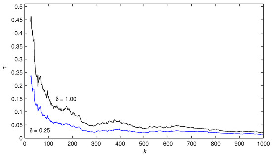
Figure 6. The estimation errors $\tau$ versus k with different noise variances for Example 2.

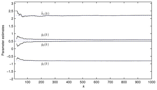
Figure 7. The parameter estimates ${\widehat{g}}_1\left(k\right)$, ${\widehat{g}}_2\left(k\right)$, ${\widehat{g}}_3\left(k\right)$ and ${\widehat{h}}_1\left(k\right)$ versus k for Example 2.

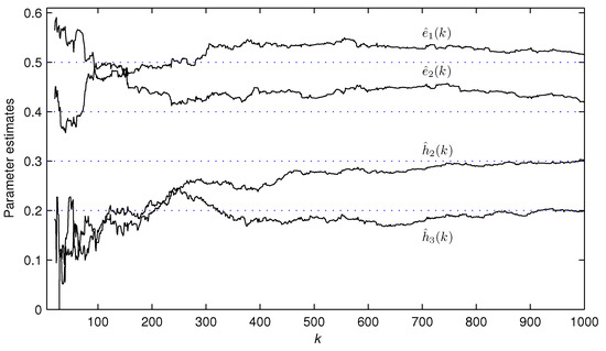
Figure 8. The parameter estimates ${\widehat{h}}_2\left(k\right)$, ${\widehat{h}}_3\left(k\right)$, ${\widehat{e}}_1\left(k\right)$ and ${\widehat{e}}_2\left(k\right)$ versus k for Example 2.

Figure 9, Figure 10 and Figure 11 plot the dynamics of three state estimates ${\widehat{\mathit{x}}}_i\left(k\right),i=1,2,3$. Figure 12 describes the output comparison of $\widehat{y}\left(k\right)$ with $y\left(k\right)$.

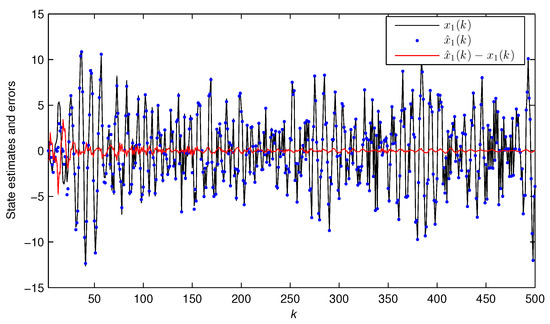
Figure 9. The true state $x_1\left(k\right)$ and the estimated state ${\widehat{x}}_1\left(k\right)$ versus k for Example 2 ($\delta =0.25$).

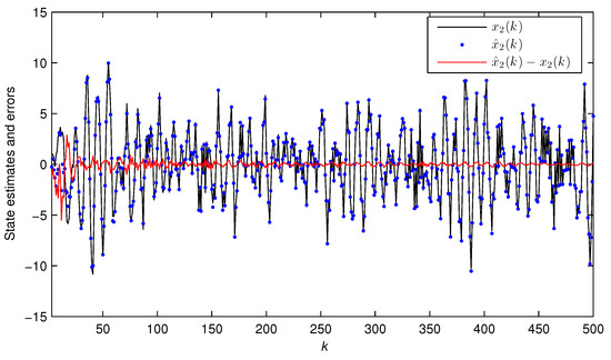
Figure 10. The true state $x_2\left(k\right)$ and the estimated state ${\widehat{x}}_2\left(k\right)$ versus k for Example 2 ($\delta =0.25$).

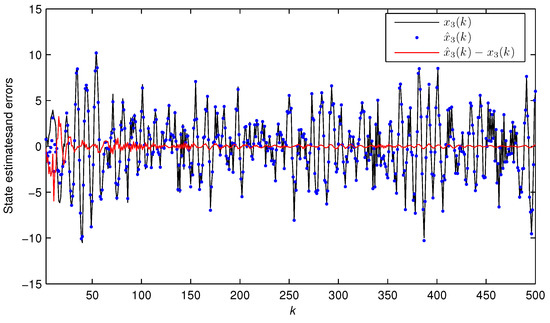
Figure 11. The true state $x_3\left(k\right)$ and the estimated state ${\widehat{x}}_3\left(k\right)$ versus k for Example 2 ($\delta =0.25$).

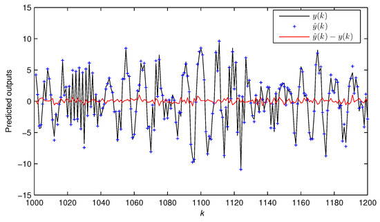
Figure 12. The actual output $y\left(k\right)$ and the estimated output $\widehat{y}\left(k\right)$ versus k for Example 2.

From Table 2 and Table 3 and Figure 1, Figure 2, Figure 3, Figure 4, Figure 5, Figure 6, Figure 7, Figure 8, Figure 9, Figure 10, Figure 11 and Figure 12, we can draw some conclusions as follows.

• The parameter estimation errors given by the BC-PSE algorithm become small with k increasing; see Table 2 and Table 3 and Figure 1 and Figure 6.
• A low noise variance leads to higher accuracy of parameter estimates; see Figure 1 and Figure 6.
• As the data length k increases, the parameter estimates approach their true values; see Figure 2, Figure 7 and Figure 8.
• The estimated states are close to the actual states of the system model; see Figure 3, Figure 4 and Figure 9, Figure 10 and Figure 11.
• The predicted outputs match well with the actual outputs; see Figure 5 and Figure 12.

5. Conclusions

This paper discusses the identification of the observability canonical state-space system with colored noise via our proposed bias compensation-based parameter and state estimation algorithm. The numerical results indicate that the algorithm can effectively estimate the system states and parameters. The advantage of this algorithm is that the parameter estimates are unbiased. The algorithm can be combined with other recursive algorithms, such as the multi-innovation algorithm, to study the identification of nonlinear state space systems [39], dual-rate systems [40], signal modeling [41] and time series analysis [42,43].

References

- Na, J.; Yang, J.; Wu, X.; Guo, Y. Robust adaptive parameter estimation of sinusoidal signals. Automatica 2015, 53, 376–384. [Google Scholar] [CrossRef]
- Kalafatis, A.D.; Wang, L.; Cluett, W.R. Identification of time-varying pH processes using sinusoidal signals. Automatica 2005, 41, 685–691. [Google Scholar] [CrossRef]
- Na, J.; Yang, J.; Ren, X.M.; Guo, Y. Robust adaptive estimation of nonlinear system with time-varying parameters. Int. J. Adapt. Control Process. 2015, 29, 1055–1072. [Google Scholar] [CrossRef]
- Liu, S.Y.; Xu, L.; Ding, F. Iterative parameter estimation algorithms for dual-frequency signal models. Algorithms 2017, 10, 118. [Google Scholar] [CrossRef]
- Na, J.; Mahyuddin, M.N.; Herrmann, G.; Ren, X.; Barber, P. Robust adaptive finite-time parameter estimation and control for robotic systems. Int. J. Robust Nonlinear Control 2015, 25, 3045–3071. [Google Scholar] [CrossRef]
- Huang, W.; Ding, F. Coupled least squares identification algorithms for multivariate output-error systems. Algorithms 2017, 10, 12. [Google Scholar] [CrossRef]
- Goos, J.; Pintelon, R. Continuous-time identification of periodically parameter-varying state space models. Automatica 2016, 71, 254–263. [Google Scholar] [CrossRef]
- AlMutawa, J. Identification of errors-in-variables state space models with observation outliers based on minimum covariance determinant. J. Process Control 2009, 19, 879–887. [Google Scholar] [CrossRef]
- Yuan, Y.; Zhang, H.; Wu, Y.; Zhu, T.; Ding, H. Bayesian learning-based model predictive vibration control for thin-walled workpiece machining processes. IEEE/ASME Trans. Mechatron. 2017, 22, 509–520. [Google Scholar] [CrossRef]
- Ding, F. Combined state and least squares parameter estimation algorithms for dynamic systems. Appl. Math. Model. 2014, 38, 403–412. [Google Scholar] [CrossRef]
- Ma, J.X.; Xiong, W.L.; Chen, J.; Ding, F. Hierarchical identification for multivariate Hammerstein systems by using the modified Kalman filter. IET Control Theory Appl. 2017, 11, 857–869. [Google Scholar] [CrossRef]
- Fatehi, A.; Huang, B. Kalman filtering approach to multi-rate information fusion in the presence of irregular sampling rate and variable measurement delay. J. Process Control 2017, 53, 15–25. [Google Scholar] [CrossRef]
- Zhao, S.; Shmaliy, Y.S.; Liu, F. Fast Kalman-like optimal unbiased FIR filtering with applications. IEEE Trans. Signal Process. 2016, 64, 2284–2297. [Google Scholar] [CrossRef]
- Zhou, Z.P.; Liu, X.F. State and fault estimation of sandwich systems with hysteresis. Int. J. Robust Nonlinear Control 2018, 28, 3974–3986. [Google Scholar] [CrossRef]
- Zhao, S.; Huang, B.; Liu, F. Linear optimal unbiased filter for time-variant systems without apriori information on initial condition. IEEE Trans. Autom. Control 2017, 62, 882–887. [Google Scholar] [CrossRef]
- Zhao, S.; Shmaliy, Y.S.; Liu, F. On the iterative computation of error matrix in unbiased FIR filtering. IEEE Signal Process. Lett. 2017, 24, 555–558. [Google Scholar] [CrossRef]
- Erazo, K.; Nagarajaiah, S. An offline approach for output-only Bayesian identification of stochastic nonlinear systems using unscented Kalman filtering. J. Sound Vib. 2017, 397, 222–240. [Google Scholar] [CrossRef]
- Verhaegen, M.; Verdult, V. Filtering and System Identification: A Least Squares Approach; Cambridge University Press: Cambridge, UK, 2007. [Google Scholar]
- Ljung, L. System Identification: Theory for the User, 2nd ed.; Prentice Hall: Englewood Cliffs, NJ, USA, 1999. [Google Scholar]
- Yu, C.P.; Ljung, L.; Verhaegen, M. Identification of structured state-space models. Automatica 2018, 90, 54–61. [Google Scholar] [CrossRef]
- Naitali, A.; Giri, F. Persistent excitation by deterministic signals for subspace parametric identification of MISO Hammerstein systems. IEEE Trans. Autom. Control 2016, 61, 258–263. [Google Scholar] [CrossRef]
- Ase, H.; Katayama, T. A subspace-based identification of Wiener-Hammerstein benchmark model. Control Eng. Pract. 2015, 44, 126–137. [Google Scholar] [CrossRef]
- Xu, L.; Ding, F.; Gu, Y.; Alsaedi, A.; Hayat, T. A multi-innovation state and parameter estimation algorithm for a state space system with d-step state-delay. Signal Process. 2017, 140, 97–103. [Google Scholar] [CrossRef]
- Zhang, X.; Ding, F.; Xu, L.; Yang, E.F. State filtering-based least squares parameter estimation for bilinear systems using the hierarchical identification principle. IET Control Theory Appl. 2018, 12, 1704–1713. [Google Scholar] [CrossRef]
- Pavelkova, L.; Karny, M. State and parameter estimation of state-space model with entry-wise correlated uniform noise. Int. J. Adapt. Control Signal Process. 2014, 28, 1189–1205. [Google Scholar] [CrossRef]
- Ma, J.X.; Wu, O.Y.; Huang, B.; Ding, F. Expectation maximization estimation for a class of input nonlinear state space systems by using the Kalman smoother. Signal Process. 2018, 145, 295–303. [Google Scholar] [CrossRef]
- Li, J.H.; Zheng, W.X.; Gu, J.P.; Hua, L. A recursive identification algorithm for Wiener nonlinear systems with linear state-space subsystem. Circuits Syst. Signal Process. 2018, 37, 2374–2393. [Google Scholar] [CrossRef]
- Wang, H.W.; Liu, T. Recursive state-space model identification of non-uniformly sampled systems using singular value decomposition. Chin. J. Chem. Eng. 2014, 22, 1268–1273. [Google Scholar] [CrossRef]
- Ding, J.L. Data filtering based recursive and iterative least squares algorithms for parameter estimation of multi-input output systems. Algorithms 2016, 9, 49. [Google Scholar] [CrossRef]
- Yu, C.P.; You, K.Y.; Xie, L.H. Quantized identification of ARMA systems with colored measurement noise. Automatica 2016, 66, 101–108. [Google Scholar] [CrossRef]
- Jafari, M.; Salimifard, M.; Dehghani, M. Identification of multivariable nonlinear systems in the presence of colored noises using iterative hierarchical least squares algorithm. ISA Trans. 2014, 53, 1243–1252. [Google Scholar] [CrossRef] [PubMed]
- Sagara, S.; Wada, K. On-line modified least-squares parameter estimation of linear discrete dynamic systems. Int. J. Control 1977, 25, 329–343. [Google Scholar] [CrossRef]
- Mejari, M.; Piga, D.; Bemporad, A. A bias-correction method for closed-loop identification of linear parameter-varying systems. Automatica 2018, 87, 128–141. [Google Scholar] [CrossRef]
- Ding, J.; Ding, F. Bias compensation based parameter estimation for output error moving average systems. Int. J. Adapt. Control Signal Process. 2011, 25, 1100–1111. [Google Scholar] [CrossRef]
- Diversi, R. Bias-eliminating least-squares identification of errors-in-variables models with mutually correlated noises. Int. J. Adapt. Control Signal Process. 2013, 27, 915–924. [Google Scholar] [CrossRef]
- Zhang, Y. Unbiased identification of a class of multi-input single-output systems with correlated disturbances using bias compensation methods. Math. Comput. Model. 2011, 53, 1810–1819. [Google Scholar] [CrossRef]
- Zheng, W.X. A bias correction method for identification of linear dynamic errors-in-variables models. IEEE Trans. Autom. Control 2002, 47, 1142–1147. [Google Scholar] [CrossRef]
- Wang, X.H.; Ding, F.; Alsaedi, A.; Hayat, T. Filtering based parameter estimation for observer canonical state space systems with colored noise. J. Frankl. Inst. 2017, 354, 593–609. [Google Scholar] [CrossRef]
- Pan, W.; Yuan, Y.; Goncalves, J.; Stan, G.B. A sparse Bayesian approach to the identification of nonlinear state-space systems. IEEE Trans. Autom. Control 2016, 61, 182–187. [Google Scholar] [CrossRef]
- Yang, X.Q.; Yang, X.B. Local identification of LPV dual-rate system with random measurement delays. IEEE Trans. Ind. Electron. 2018, 65, 1499–1507. [Google Scholar] [CrossRef]
- Xu, L.; Xiong, W.L.; Alsaedi, A.; Hayat, T. Hierarchical parameter estimation for the frequency response based on the dynamical window data. Int. J. Control Autom. Syst. 2018, 16, 1756–1764. [Google Scholar] [CrossRef]
- Gan, M.; Chen, C.L.P.; Chen, G.Y.; Chen, L. On some separated algorithms for separable nonlinear squares problems. IEEE Trans. Cybern. 2018, 48, 2866–2874. [Google Scholar] [CrossRef] [PubMed]
- Chen, G.Y.; Gan, M.; Chen, G.L. Generalized exponential autoregressive models for nonlinear time series: Stationarity, estimation and applications. Inf. Sci. 2018, 438, 46–57. [Google Scholar] [CrossRef]
© 2018 by the authors. Licensee MDPI, Basel, Switzerland. This article is an open access article distributed under the terms and conditions of the Creative Commons Attribution (CC BY) license (http://creativecommons.org/licenses/by/4.0/).