K-Means Cloning: Adaptive Spherical K-Means Clustering


1
Department of Computer Science, Faculty of Comp. & Info, Assiut University, Assiut 71526, Egypt
2
Department of Computer Science in Jamoum, Umm Al-Qura University, Makkah 25371, Saudi Arabia
3
Department of Mathematics, Faculty of Science, Al-Azhar University, Assiut Branch, Assiut 71524, Egypt
4
Electrical Engineering Department, Assiut University, Assiut 71516, Egypt
*
Author to whom correspondence should be addressed.
Algorithms 2018, 11(10), 151; https://doi.org/10.3390/a11100151
Submission received: 17 May 2018
/
Revised: 22 September 2018
/
Accepted: 25 September 2018
/
Published: 6 October 2018
Abstract
:We propose a novel method for adaptive K-means clustering. The proposed method overcomes the problems of the traditional K-means algorithm. Specifically, the proposed method does not require prior knowledge of the number of clusters. Additionally, the initial identification of the cluster elements has no negative impact on the final generated clusters. Inspired by cell cloning in microorganism cultures, each added data sample causes the existing cluster ‘colonies’ to evaluate, with the other clusters, various merging or splitting actions in order for reaching the optimum cluster set. The proposed algorithm is adequate for clustering data in isolated or overlapped compact spherical clusters. Experimental results support the effectiveness of this clustering algorithm.
1. Introduction
Data mining is a helpful and efficient process for analysis and implementation of data. Cluster analysis could be defined as uncensored data classification, it is a crucial topic in data mining [1]. It aims at attempting to partition a collection of patterns into groups (clusters) of similar data points. Patterns within a cluster are more similar to each other than patterns belonging to other clusters. Clustering methods [2] have been involved in many applications, including information retrieval, pattern classification, document extraction, image segmentation, etc.
Data clustering techniques can be broadly divided into two groups: hierarchical and partitional [1,3,4]. Hierarchical clustering techniques is a tree showing a sequence of clustering. Hierarchical algorithms can be agglomerative (bottom-up) mode starting with each instance in its own cluster and merging the most similar pair of clusters successively to form a cluster hierarchy; or in divisive (top-down) mode starting with all the instances in one cluster and recursively splitting each cluster into smaller clusters. Partitional clustering methods find all the clusters simultaneously as a partition of the data without any other subpartition like hierarchical structures do and are often based on the combinatorial optimization task of the best configuration of partitions among all possible ones, according to a function that assesses the quality of partitions (objective function). In this paper we will consider partition clustering.
In the field of clustering, the K-means algorithm [5,6,7] is one of the most popular clustering techniques for finding structures in unlabeled datasets. It can be used to partition a number of data points into a given number of clusters, which is based on a simple iterative scheme for finding a local minimum solution. The K-means algorithm is well known for its efficiency and its ability to cluster large datasets. However, a major bottleneck in the operation of K-means is the requirement of predefinition of the clusters number [8]. From another side, the high dependence of the final clustering on the initial identification of clusters elements represents another difficulty to the operation of K-means [8].
Some research studies have approached the clustering problem from a meta-heuristic perspective. Meta-heuristics have a major advantage over other methods, which is the ability to avoid becoming trapped at local minima. Such algorithms exploit guided random search. Therefore, much better results have been obtained with meta-heuristics approaches, such as simulated annealing [9,10,11,12,13,14], tabu search [15,16], and genetic algorithms [17]. They combine techniques of local search and general strategies to escape from local optima leading to broadly searching the solution space. The objective of such combination is to obtain solutions that are closer to the global optima (centroids) of the clusters. Based on the tendency of the K-means algorithm to obtain local optima [18], this work investigates a new approach to solve clustering problem.
Data clustering is known to be NP hard in finding groups in heterogeneous data [19]. It is the process of grouping similar data items together based on some measure of similarity (or dissimilarity) between items. A major difficulty that exists with K-means clustering, as one of the most well-known unsupervised clustering methods, is the requirement of prior knowledge about the number of clusters. This piece of information could be difficult to know in advance for many applications. Moreover, K-means has other well-known drawbacks, sensitivity to initial configuration and its convergence to local optima. These problems are raised in the literature, see [7,20,21,22,23,24,25] and reference therein. Different treatments have been discussed to find better tuning mechanisms of the number K including statistical tests, probabilistic models, incremental estimation process, or visualization schemes. In the following, we give a brief presents of some of those treatments.
In [26], the authors built a powerful learning-based fuzzy C-means structure, so it turns out to be free of the fuzziness index m and initializations without parameter choice, and can likewise consequently locate the best number of clusters. They initially utilized entropy-type penalty terms for optimizing the fuzziness index, and afterward make a learning-based schema for finding the best number of clusters. That learning-based schema uses entropy terms contain the belonging probabilities of data points to clusters and the average of occurrence in those probabilities over fuzzy memberships to find the best number of clusters.
Kuo et al. [27] proposed a new automatic clustering approach based on particle swarm optimization and genetic algorithm. Their algorithm can automatically find data clusters by examining the data without need to set a fixed number of clusters. Specifically, the number of clusters is treated as a variable to be optimized within the clustering method.
In [28], the authors proposed an intelligent K-means method, called -means, that locates the number of clusters by extracting odd examples from the data one-by-one. They used the Gaussian distribution to generate cluster models. Therefore, the clustering process can be analyzed through the usage of Gaussians in the data generation and specifics K-means clusters. Then, they could compare the performance of methods in terms of their capabilities in recovering cluster centroids as well as their abilities to recover of the number of clusters or clusters themselves. Their final version of -means utilizes the cluster number tuning, the cluster recovery, and the centroid recovery.
Hamerly and Elkan [29] proposed the G-means algorithm, which is based on assuming a statistical test checking if a subset of data follows a Gaussian distribution or not. G-means implements K-means with increasing values of K in a hierarchical structure until the hypothesis test is accepted.
The authors of [30] presented a projected Gaussian method for data clustering called -means. Their method tries to discover an appropriate number of Gaussian clusters, as well as their positions and orientations. Therefore, their clustering strategy inherits the features of the well-known Gaussian mixture model. The main contribution of that paper is to use projections and statistical tests to determine if a generated mixture model fits its data or not.
Tibshirani et al. [31] introduced a new measurement to estimate the number of clusters based on comparing the change within-cluster dispersion through some statistical tests. That measure can be used to the output of any clustering method in order to adapt the number of clusters.
Kurihara and Welling [32] presented a Bayesian K-means based on the mixture model learning using the expectation-maximization method. Their method can be implement as a top-down approach “Bayesian k-means” or as a bottom-up one “agglomerative clustering”.
In [33], Pelleg et al. introduced a new algorithm, X-means, to find the best configuration of the cluster locations and the number of clusters to optimize the Bayesian or Akaike information criteria. In each K-means run, the current centroids should be checked by the splitting conditions using Bayesian information criterion. A modified version of the X-means algorithm is presented in [34]. The main deviation is to apply a new cluster merging procedure to avoid unsuitable splitting caused by the cluster splitting order.
Pham et al. [23] presented an extensive review of the existing methods for selecting the number of clusters in K-means algorithms. In addition, the authors introduced a new measure to evaluate the selection of the number K.
In [35], the authors proposed a new clustering technique based on a modified version of K-means and a union-split algorithm to find a better value of the number of clusters. Those clustering methods are applied to undirected graphs to cluster similar graph nodes into clusters with a minimum size constraint to the cluster number.
Other studies followed dynamic clustering strategies, e.g., in [36], cluster combination is performed using an evidence accumulation approach. Also Guan et al. [37] have developed Y-means as an alternative clustering method of K-means. In Y-means, the number of clusters can be dynamically determined via assigning or removing data points to or from generated clusters depending on an Eacludian metric.
Masoud et al. [38] proposed a dynamic data clustering method based on the combinatorial particle swarm optimization technique. Their method treats the data clustering problem as a single problem, including the sub-problem of finding the best number of clusters. Therefore, they tried to find the number of clusters and cluster centers simultaneously. In order to adapt the number of clusters, a similarity degree between the clusters is computed and the clusters with the highest similarity are merged.
The authors of [39] developed a new method for automatically determination of the number of clusters based on some existing image and signal processing algorithms. Their algorithm generates an image representation of the data dissimilarity matrix and converts it to a Laplacian matrix. Then, visual assessment of cluster tendency techniques is applied in the latter matrix after normalizing its rows.
Metaheuristics are powerful and practical tools that have been applied to many different problems [40,41]. Many clustering methods have been designed as metaheuristic-based methods [42,43,44]. Such methods try to find global optimal configurations of data clusters within reasonable processing times. Different types of metaheuristics have been used to solve different data clustering problems such as genetic algorithms [45,46,47,48,49,50,51], simulated annealing [18,52,53], tabu search [54,55], particle swarm optimization [54,56,57,58,59], ant colony optimization [60,61,62,63], harmony search algorithm [64,65], and firefly algorithm [66,67].
Most of the above-mentioned papers mainly use statistical tests, probabilistic models, incremental estimation process, or visualization schemes. These procedures are usually deteriorated when applied to complex or big data sets. Therefore, we propose K-Means Cloning (KMC) algorithm as a dynamic clustering approach that generates continuously evolving clusters as new samples are added to the input dataset; the case which makes it very adequate to real-time fed data streams and for large datasets whose unpredictable number of clusters.
This paper describes KMC and its application to the automatic clustering of large unlabeled data sets. In contrast to most of the existing clustering techniques, the proposed algorithm requires no prior knowledge of the data to be classified. Rather, it determines the optimal number of partitions of the data with consistency of the results in every runs. KMC generates dynamic “colonies” of K-means clusters. As data samples are added to the dataset the initial number of clusters as well as the clusters structures are modified for the sake of achieving optimality constraints. The structure of the iteratively-generated clusters is changed using intensification and diversification of the K-means cluster. Superiority of the new method is demonstrated by comparing it with some state-of-the-arts clustering techniques.
The rest of this paper is organized as follows. In Section 2, the outlines of the proposed K-means cloning are described. Necessary overview of the used simulated annealing approach as well as the problem modeling are explained. Section 3 shows how the procedure ingredients are used to build up the entire KMC algorithm. Experimental setup is detailed in Section 4. A comprehensive discussion of the obtained evaluation results is presented in Section 5. Finally, the paper is concluded in Section 6.
2. K-Means Cluster Cloning
The proposed KMC data clustering procedure involves three main processes: the first one is measuring the similarity/dissimilarity between a data sample and the existing clusters in the data spaces. The second process is taking a decision of merging two existing clusters into a larger one, if they achieved a specific merging similarity constraint. The third is conducted if some degree of dissimilarity is reached within an existing cluster. In this case, the cluster is split into two or more smaller clusters. All of these three processes are performed in an integrated fashion in order for achieving global optimality conditions. Therefore, we look at this problem as a global search problem from an optimization perspective. Within this search, an optimum point in the search space, whose independent variables are the number of clusters and the data samples’ memberships to the constructed clusters, is to be found.
The problem, as described in this context of the size and discontinuity of the search space, stimulates the usage of meta-heuristic search. We opted to use simulated annealing for this purpose. However, the problem can be remodeled to accommodate any other meta-heuristic approach.
In the next subsection, we give a brief review of the SA algorithm. Then, in the following subsections, we describe the proposed model incorporating the aforementioned three processes.
2.1. Simulated Annealing Heuristic
Simulated Annealing (SA) [68] is a generic probabilistic meta-heuristic for the global optimization problem of locating a good approximation to the global optimum of a given function in a large search space. It is a random-search technique and often used when the search space is discrete. For certain problems, simulated annealing may be more efficient than exhaustive enumeration provided that the goal is merely to find an acceptably good solution in a fixed amount of time, rather than the best possible solution.
SA, as its name implies, exploits an analogy between the way in which a metal cools and freezes into a minimum energy crystalline structure, i.e., the annealing process. The SA algorithm successively generates a trial point in a neighborhood of the current solution and determines whether or not the current solution is replaced by this trial point based on a probability value. This value is related to the difference between their function values. Convergence to an optimal solution can theoretically be guaranteed only after an infinite number of iterations controlled by the procedure so-called cooling schedule. Algorithm 1 describes the main algorithmic steps of simulated annealing.
For global search purposes, it does not only accept changes that decrease the objective function f (assuming a minimization problem), but also it makes some changes that increase it. The latter are accepted with a probability;
where is the increase in f and T is a control parameter, which by analogy with the original application is known as the system “temperature” irrespective of the objective function involved.
| Algorithm 1 Simulated Annealing |
|
SA has been used on a wide range of combinatorial optimization problems and achieved good results. In data mining, SA has been used for feature selection, classification, and clustering [69].
2.2. Clusters’ Fitness Function
To measure the quality of the proposed clustering, we exploit the silhouette as a fitness function [70,71,72,73]. In order to calculate the final silhouette fitness function, two inputs should be firstly computed for all data objects as shown in the following.
- Inner Dissimilarity (): is the average dissimilarity between a data object i and other objects in its cluster , which can given bywhere is the classical Euclidean distance used in K-means, and is the number of objects in cluster .
- Outer Dissimilarity (): is the minimum distance between a data object i to cluster centers except its cluster , this can be computed in two steps as follows. First, we compute the average dissimilarity () between i and other cluster ,where is the number of objects in cluster . Then, can be computed as,
From Equation (1), the cluster silhouette is the average dissimilarity of its data objects.
Finally, the clusters fitness function is the average of all cluster silhouettes.
It is worthwhile to mention that the object dissimilarity satisfies the condition,
This condition is still valid for and since they are computed as averages of . Moreover, each different value of K generates a different . The higher value can achieve, the better clustering can be obtained.
2.3. K-Means Colony Growth
A major challenge in partitional clustering lies in determining the number of clusters that best characterize a set of observations. The question is: In starting with an initial number of clusters, what mechanism through which the search strategy can find the best solution, i.e., actual number clusters? To answer this question we define the cluster merging and splitting procedures which are discussed in this section.
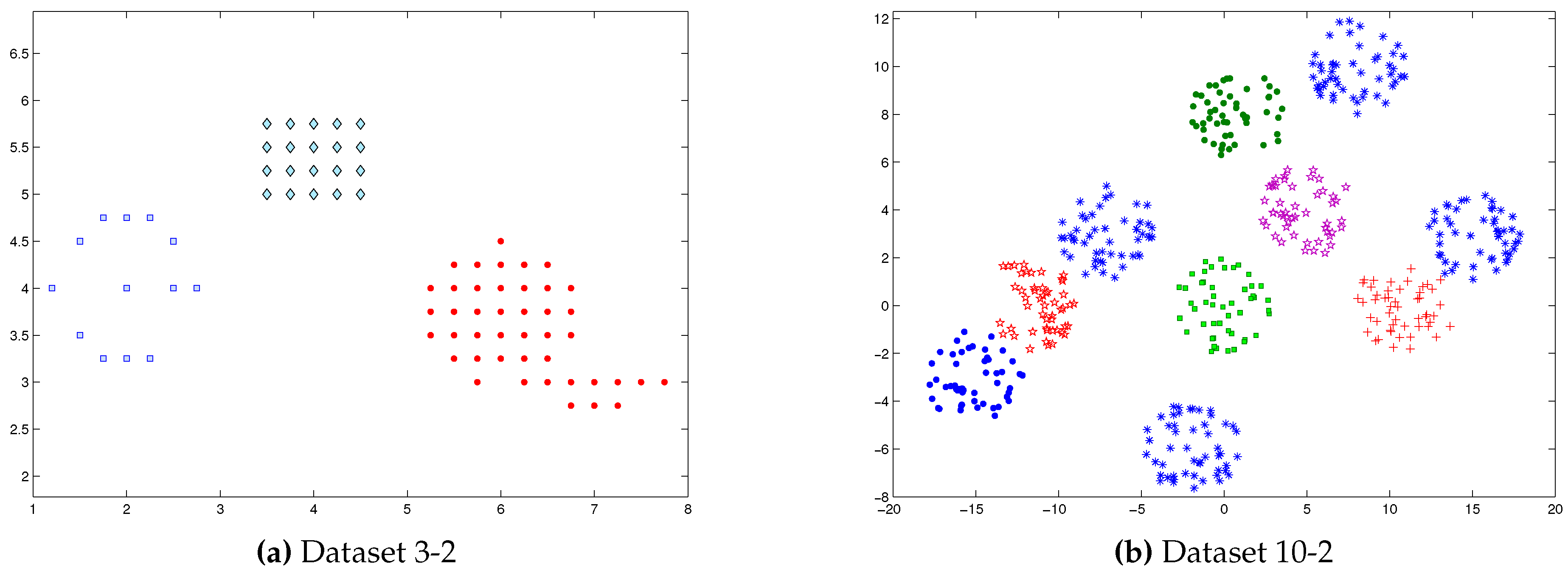
For further explanation, we used two synthetic datasets described as follows:
The adaption process to fix the number of clusters depends on three sub-processes; how to evaluate the current number of cluster, which cluster(s) should be split or merged, and how we perform the cluster splitting or merging. These sub-processes are discussed in the following.
2.3.1. Evaluating the Number of Clusters
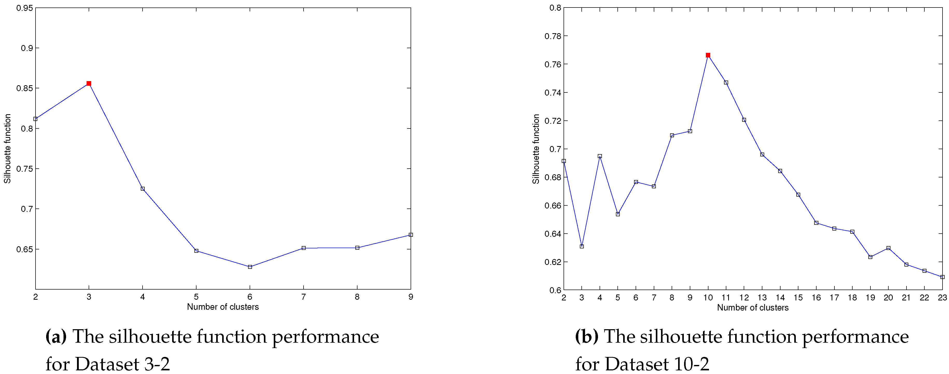
It is instructive to see how clustering objective function changes with respect to the change of K, the number of clusters. During our experiments, we discovered that the performance of measure moves towards the best solution (optimum number of clusters) smoothly. was sequentially applied to several dataset with the number of clusters ranging from 2 to . SA was run many times starting with initial fixed number , using Dataset 3-2 and Dataset 10-2. The best values obtained with maximum measure were stored. The final outcome of these calculations and the performance of are shown in Figure 2.
In Figure 2a the peak begin when and minimum , then starts increasing with the increase of the number of clusters and together for Dataset 3-2. continues to increase until it reaches the maximum value when the maximum peak is reached for = 0.856. Then, begin to decline with continued increase of the number of clusters. Similarly, the maximum peak for the Dataset 10-2 is reached when = 0.7664, as shown in Figure 2b.
These obtained values comply with the common sense evaluation of the data by visual inspection. Also the well-known Ruspini dataset [72], has been widely used as a benchmark for clustering algorithms, the maximum peaks are achieved when , see [71]. We need two values for the number of clusters, the initial number K and random with two values. By comparing the two values for two values of number clusters, the next step whether of merging or splitting process is determined. The following procedure illustrates this process.
Procedure 1.
K-Adaptation
- 1.
- Input: two clustering outputs and with and clusters, respectively, with .
- 2.
- If , then apply cluster merging (Procedure 2) or cluster splitting (Procedure 3) randomly in order to get different cluster numbers. Rename the obtained clusters to ensure that .
- 3.
- Evaluation: compute and .
- 4.
- Merging: if , then apply cluster merging (Procedure 2) on , to produce clusters. Set , and return.
- 5.
- Splitting: if , then apply cluster splitting (Procedure 3) on , to produce clusters. Set , and return.
- 6.
- Neutral: randomly apply the cluster merging or splitting procedure on or to produce new clusters, and return.
Accordingly, a decision is taken using SF by either merging two smaller clusters into a larger one or splitting a larger cluster into smaller ones.
2.3.2. Split/Merge Decision
A crucial step is how to select the next cluster(s) to split or merge. Our splitting and merging procedures issue criterion functions to select cluster(s) to be split or merged according to fitness assessments on the changing cluster structure. It is instructive to see how clustering objective functions change with respect to the change of the number of clusters K. The idea of performing split and merge procedures has been successfully applied to calculating the cluster silhouettes . If the decision was splitting, the cluster which has the minimum cluster silhouette is the one to be split into two sub-clusters. On the other hand, if the decision was merging, the two clusters with minimum cluster silhouettes are the two to be merged.
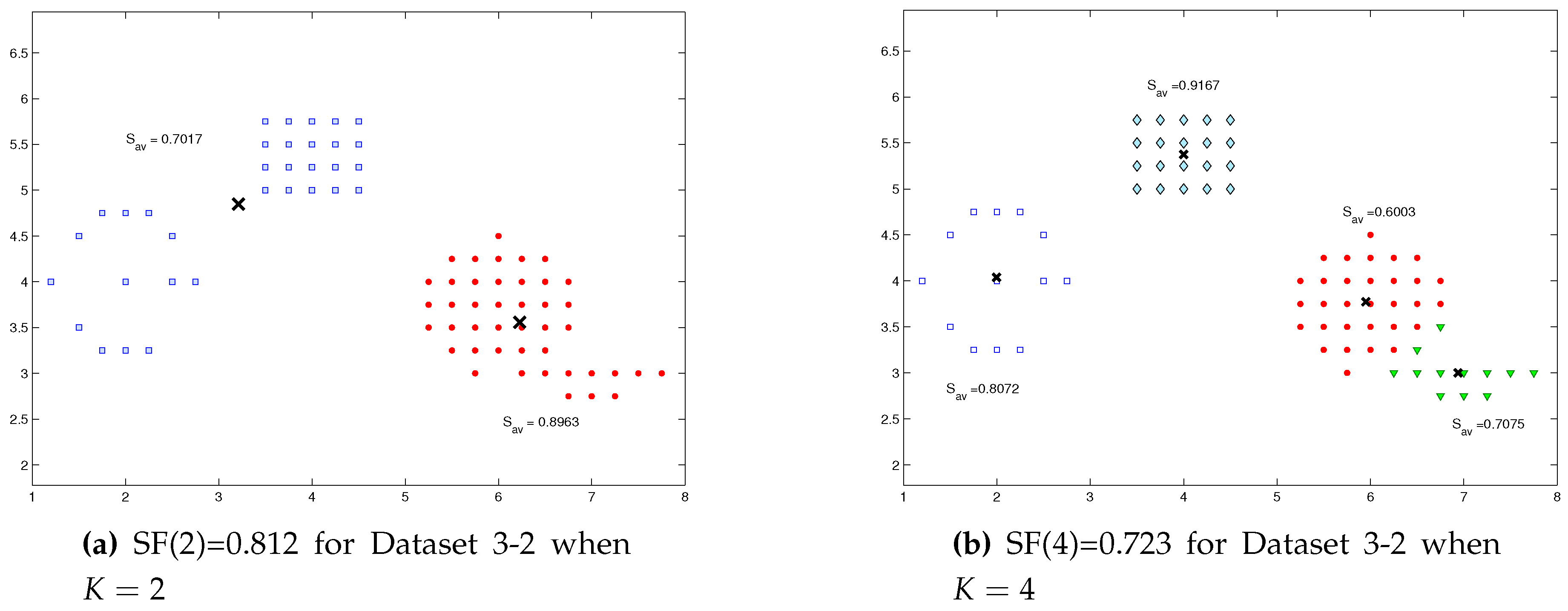
As an illustrative example, Dataset 3-2 in Figure 1a has the largest value of , with the optimal number of cluster , as also shown in Figure 2a. We computed two appropriate clusters for Dataset 3-2, which and , as shown in Figure 3a. Similarly, four appropriate clusters for the same Dataset 3-2, which are , , and , see Figure 3b. According to the K-Adaptation Procedure, if the comparison was between and and , then splitting procedure must be applied to the cluster which have the minimum dissimilarity , as shown in Figure 3a. In the case of which the comparison was between and and , merging procedure must be applied to the two clusters whose the minimum dissimilarities , as shown in Figure 3b.
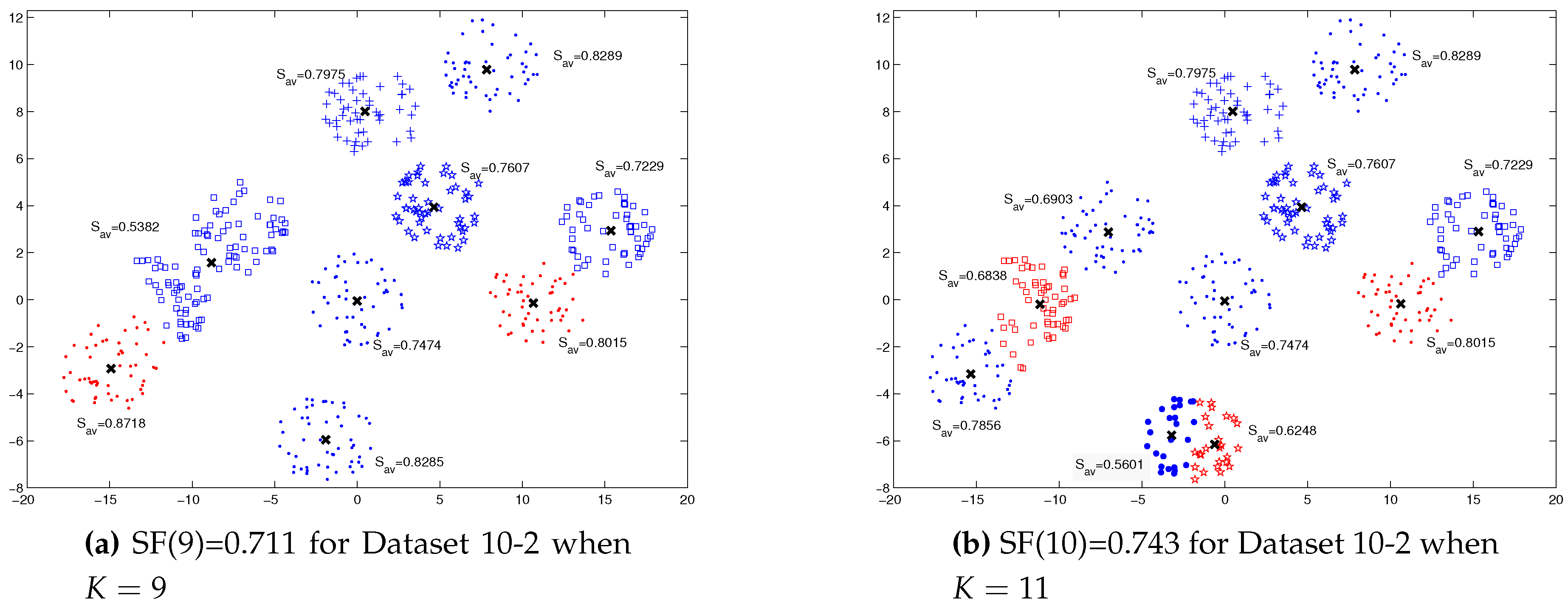
For Dataset 10-2, Figure 4 describes how the split/merge decision is taken for the clusters that need to be split are determined, as in Figure 4a, or merged, as in Figure 4b.
Many attempts were performed on other datasets and proved the veracity of this method and adoption of it as a cluster merging and splitting method to detection an appropriate clusters.
2.3.3. How to Split or Merge
K-means cloning is a continuous evolving process that is represented by split and merge of K-means clusters. Merging and Splitting Procedures 2, 3 show the cloning mechanism of merging two clusters into a larger one, and how a single cluster is split into two new clusters with new centers. When a cluster is split into two sub-clusters, new-alternative centers are generated.
Procedure 2.
Merging
- 1.
- Input: clustering outputs with clusters , and for each cluster is the number of objects in this cluster, and his center is .
- 2.
- Evaluate the cluster silhouettes .
- 3.
- Sort the cluster silhouettes to determine the two clusters with the minimum cluster silhouettes and .
- 4.
- Set a new center as,
- 5.
- Replace the centers and by , set .
- 6.
- Adjust the new generated centers based on K-means, and return with the adjusted clusters.
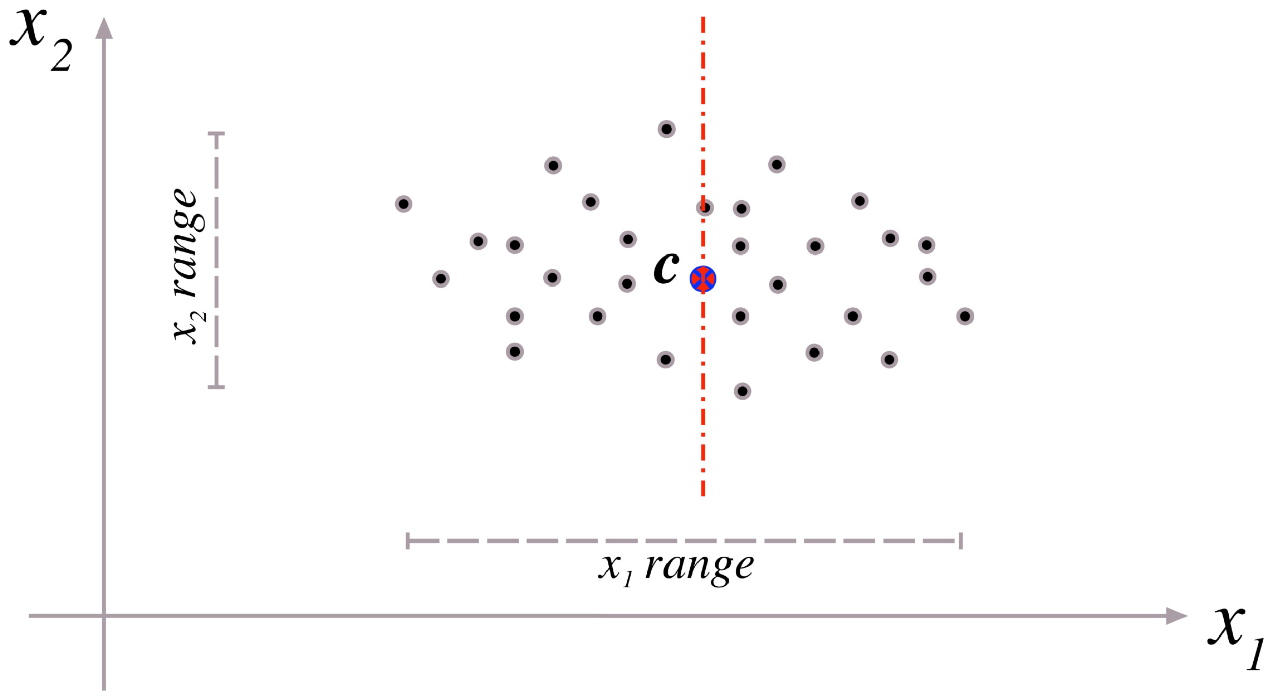
The splitting process is applied to the cluster with the minimum cluster silhouette value among all clusters. A hyperplane is generated to split this cluster objects in order to generate two new clusters. Coordinate-wise variances are computed over the data objects of the chosen cluster. Then, the separation hyperplane is generated passing through the cluster center and orthogonal to the coordinate axis corresponding to the highest variance component of the data objects. Figure 5 shows an example of cluster splitting in two dimensions. In this figure, it is clear that the data variance over -axis is higher than that over -axis. Therefore, the dashed hyperplane is generated passing through center c and orthogonal to -axis in order to separate the data objects into two clusters along the both sides of the hyperplane. Data objects which are located on the hyperplane can be added to any of the two clusters since new centers will be computed and all data objects will be adjusted as in the case of K-means.
Procedure 3.
Splitting
- 1.
- Input: clustering outputs with clusters , and for each cluster is the number of objects in this cluster, and his center is .
- 2.
- Evaluate the cluster silhouettes .
- 3.
- Sort the cluster silhouettes to determine the cluster with the minimum cluster silhouette.
- 4.
- Divide cluster into two sub-clusters with objects and by splitting the data objects in using a separation hyperplane passing through its center and orthogonal to the coordinate axis corresponding to the highest variance component of the data objects.
- 5.
- Compute the centers and of the new clusters and , respectively.
- 6.
- Replace with and , set .
- 7.
- Adjust the new generated centers based on K-means, and return with the adjusted clusters.
2.4. Diversification
In the proposed KMC method, we use a diversification generation method to generate a diverse solution. This diverse solution can help the search process to scape from local minima. The search space of the parameter K, which is the interval , is divided into equal sub-intervals. When a predefined consecutive number of iterations is reached without hitting any of these sub-intervals, a new diverse solution should be generated from the unvisited sub-intervals. In order to generate a new diverse solution, a new value of is randomly chosen from the unvisited sub-intervals and the K-means clustering process is implemented to compute new clusters , . Procedure 4 formally explains the steps of the diversification process.
Procedure 4.
Diversification
- 1.
- Input: the lower and upper bounds and of the number of clusters, respectively, the number of cluster number sub-intervals, and numbers of visiting each sub-interval.
- 2.
- Select an η from with a probability inversely proportional to its corresponding visiting number .
- 3.
- Choose a randomly from the selected sub-interval η.
- 4.
- Generate new centers.
- 5.
- Adjust the generated centers based on K-means, and return with the adjusted clusters.
3. KMC Algorithm
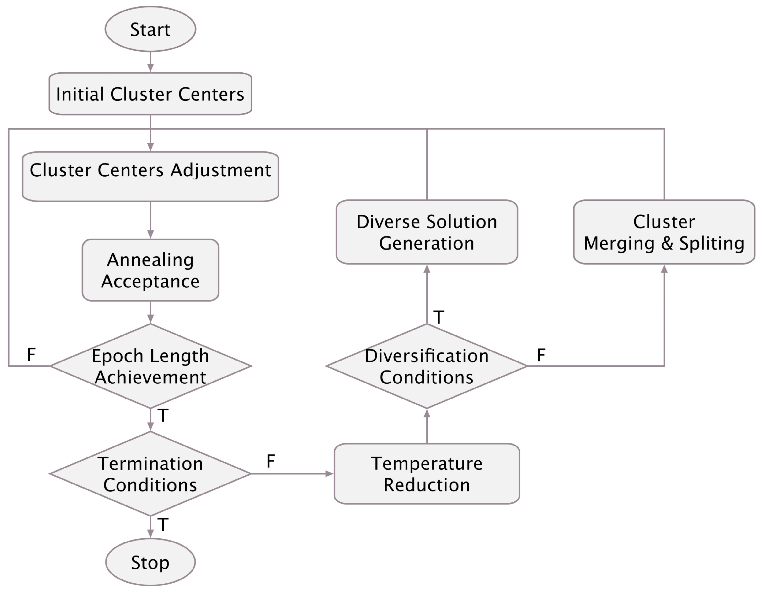
In this section, we outline the KMC algorithm. We show how the algorithm exploits the aforementioned cluster number determination, splitting, and merging procedures to perform K-means evolving cloning. The details of the proposed method is given in Algorithm 2. Moreover, a general layout of the algorithm is shown in Figure 6.
| Algorithm 2 KMC |
|
Using KMC, the accurate number of clusters can be found automatically with reasonable runtime and acceptable competing accuracy. The epoch length is responsible for determining the best centers for number of clusters, the split and merge procedure issues criterion functions to select clusters to be split or merged, and fitness assessments on cluster structure changes.
4. Experimental Setup
In this section, the comparison strategy of KMC algorithm is described. We describe how the parameters were set and the comparisons were conducted. Also, brief descriptions of the datasets and the algorithms used in comparisons are presented.
4.1. Test Bed
To evaluate the performance of the proposed algorithm, five synthetic and two real datasets. The real datasets extracted from UCI public data repository [75]. Table 1 presents the number of instances, attributes and the number of clusters of each dataset.
- Separate 3: This dataset was produced by sampling outputs with normal distributions from a cluster generator. It consists of 150 two dimensional data points distributed over three spherically-shaped clusters. The clusters are highly overlapping, each consists of 50 data points. This dataset is shown in Figure 7a.
- Overlap 3: It is similar to Separate3 except it is in three-dimensional space and distributed over four hyper-spherical disjoint clusters. Each cluster contains 50 data points. This dataset is shown in Figure 7b.
- Iris: This dataset consists of 150 data points distributed over three clusters [77]. Each cluster has 50 points. This dataset represents different categories of irises characterized by four feature values. It has three classes Setosa, Versicolor and Virginica. It is known that two classes (Versicolor and Virginica) have a large amount of overlap, while the class Setosa is linearly separable from the other two.
- Breast cancer: This Wisconsin Breast Cancer dataset consists of 683 sample points. Each pattern has nine features corresponding to clump thickness, cell size uniformity, cell shape uniformity, marginal adhesion, single epithelial cell size, bare nuclei, bland chromatin, normal nucleoli and mitoses. There are two categories in the data: malignant and benign. The two classes are known to be linearly separable.
4.2. Parameter Setting and Tuning
The KMC algorithm was programmed in MATLAB and its parameters are set according to their standard setting or our preliminary experiments. The details of setting these parameter are given as follows. The cooling schedule consists of the initial temperature , the cooling function, the epoch length M and the stopping condition. We choose the value of large enough to make the initial probability of accepting transition close to 1. We set the initial probability to 0.9. Then, is calculated from the equation . The temperature is reduced from , where is a parameter called cooling ratio. Epoch length M is the number of trials allowed at each temperature and we set it to 8. Initial number of clusters is chosen between , where number of points, and . We have observed that the diversification and intensification procedure is more effective when setting . The stopping condition is satisfied when a minimum allowed temperature is hit. The parameter setting values are summarized in Table 2.
4.3. Numerical Comparisons
We first provide the results obtained over the aforementioned three well-chosen synthetic datasets Overlap 5, Separate 6 and Separate 4, shown in Figure 7 and the real dataset breast cancer used on [17]. The performance of KMC has been compared with: the MEPSO [78] algorithm based on a modified the Particle Swarm Optimization (PSO) algorithm with improved convergence properties, the fuzzy c-means (FCM) [79] algorithm, which is the most popular algorithm in the field of fuzzy clustering. The later algorithm is referred in literature as Fuzzy clustering with Variable length Genetic Algorithm (FVGA) [17].
Then, we provide the results obtained over four synthetic datasets Separate 3, Overlap 3, Overlap 5 and Separate 6, shown in Figure 7, and iris dataset. The first two datasets are produced by sampling from normal distributions with a cluster generator, and the other two datasets used in previous performance shown in Figure 7c,d. We used ten instances of each of the dataset Overlap 3 in our evaluation and multiple runs were distributed evenly across the instances. We compare the performance of KMC with a cooperative co-evolutionary algorithm (CCEA) and a variable string-length GA (VGA) [17,80,81].
5. Results and Discussions
The clustering results of the KMC algorithm are shown in Table 3 and Table 4. Two major indicators of performance can be found in these tables: the average computed number of clusters and the average classification error, accompanied by the corresponding standard deviations.
In Table 3, we took twenty independent runs and provided the mean value and standard deviation evaluated over final clustering results for each algorithm. The number of classes evaluated and the number of misclassified items with respect to the known partitions and classification objects are reported. We can see from the results that are presented in this table, on synthetic and real datasets, all computed clusters that were obtained from the KMC algorithm exactly equals the ground truth classes without any deviation at all runs. Furthermore, KMC obtains misclassification error rates zero in two of datasets.
In Table 4, the results are averaged over 50 runs on each of the evaluation datasets. Specifically, we used ten instances of each of these datasets in our evaluation and multiple runs were distributed evenly across the instances. Table 4 shows the comparison results of KMC with CCEA and VGA using Overlap 3, 5 and Separate 3, 6 synthetic datasets, as well as the Iris real datasets. The class distribution is presented in Table 5. As it is seen from the table, the exact real number of classes have been obtained by KMC algorithm without any deviation. Both CCEA and VGA have deviations in the number of classes with or more datasets.
In most real datasets the number of clusters is not priori known. So, to illustrate the potential of KMC in accurate estimation of the number of clusters in non-obvious datasets, KMC was applied to ten well-known real datasets [75].
In order to test the performance of the proposed method in higher dimensional datasets, two datasets called “Hill-Valley” and “LSVT” are used [75]. The details of these datasets are given in Table 6. The KMC method could obtained the exact number of cluster for both datasets as stated in Table 6. Figure 8 shows the performance of the KMC method in improving the misclassification errors for these datasets. The average misclassification errors for Hill-Valley and LSVT datasets are 14.95% and 27.98%, respectively.
Finally, we present the cluster analysis figures to show how the proposed algorithm could distribute points over clusters. Figure 9 and Figure 10 show that for low dimensional datasets, while Figure 11 illustrates the point distributions for big datasets. Those figures show the efficiency of the proposed method in assigning the right clusters for the majority of points in different datasets.
6. Conclusions
In this paper, we have introduced K-Means Cloning (KMC) as an adaptive clustering approach that is based on K-means clustering. It is a reliable evolving clustering technique that comprises two novel merging and splitting procedures. KMC uses meta-heuristics global search that is based on the silhouette function. Experiments on synthetic and real datasets proved the potential of KMC in accurate estimation of the number of clusters and as an adaptive clustering method.
Author Contributions
Conceptualization, A.-R.H., A.-M.I., A.E.A.-H., A.A.S.; Methodology, A.-R.H., A.-M.I., A.E.A.-H., A.A.S.; Programming & Coding, A.-R.H., A.-M.I.; Writing-original Draft Preparation, A.-R.H., A.-M.I.; Writing-review & Editing, A.-R.H., A.E.A.-H., A.A.S.; Visualization, A.-R.H., A.E.A.-H.; Funding Acquisition, A.E.A.-H.
Funding
This work was supported by the Deanship of Scientific Research at Umm Al-Qura University, Grant No. 15-ENG-3-1-0012
Acknowledgments
The authors would like to thank the Deanship of Scientific Research at Umm Al-Qura University for the continuous support. This work was supported financially by the Deanship of Scientific Research at Umm Al-Qura University to Alaa E. Abdel-Hakim—(Grant Code: 15-ENG-3-1-0012).
Conflicts of Interest
The authors declare no conflict of interest.
References
- Berkhin, P. A survey of clustering data mining techniques. In Grouping Multidimensional Data; Springer: Berlin/Heidelberg, Germany, 2006; pp. 25–71. [Google Scholar]
- Xu, R.; Wunsch, D. Survey of clustering algorithms. IEEE Trans. Neural Netw. 2005, 16, 645–678. [Google Scholar] [CrossRef] [PubMed]
- Leung, Y.; Zhang, J.; Xu, Z. Clustering by scale-space filtering. IEEE Trans. Pattern Anal. Mach. Intell. 2000, 22, 1396–1410. [Google Scholar] [CrossRef]
- Ward, J. Hierarchical grouping to optimize an objective function. J. Am. Stat. Assoc. 1963, 58, 236–244. [Google Scholar] [CrossRef]
- Bagirov, A.M. Modified global K-means algorithm for minimum sum-of-squares clustering problems. Pattern Recognit. 2008, 41, 3192–3199. [Google Scholar] [CrossRef]
- Hammerly, G.; Elkan, C. Alternatives to the K-means algorithm that find better clusterings. In Proceedings of the Eleventh International Conference on Information and Knowledge Management, McLean, VA, USA, 4–9 November 2002; pp. 600–607. [Google Scholar]
- Jain, A.K. Data clustering: 50 years beyond K-means. Pattern Recognit. Lett. 2010, 31, 651–666. [Google Scholar] [CrossRef] [Green Version]
- Bhatia, S.K. Adaptive K-Means Clustering. In Proceedings of the FLAIRS Conference, Miami Beach, FL, USA, 2004; pp. 695–699. [Google Scholar]
- Agard, B.; Penz, B. A simulated annealing method based on a clustering approach to determine bills of materials for a large product family. Int. J. Prod. Econ. 2009, 117, 389–401. [Google Scholar] [CrossRef]
- Al-Harbi, S.H.; Rayward-Smith, V.J. Adapting k-means for supervised clustering. Appl. Intell. 2006, 24, 219–226. [Google Scholar] [CrossRef]
- Das, S.; Abraham, A.; Konar, A. Metaheuristic Clustering; Springer: Berlin/Heidelberg, Germany, 2012. [Google Scholar]
- Laarhoven, P. Theoretical and Computational Aspects of Simulated Annealing; Stichting Mathematisch Centrum: Amsterdam, The Netherlands, 1988. [Google Scholar]
- Laarhoven, P.; Aarts, E. Simulated Annealing: Theory and Applications; Mathematics and Its Applications; Springer: Dordrecht, The Netherlands, 2010. [Google Scholar]
- Mohamadi, H.; Habibi, J.; Abadeh, M. Data mining with a simulated annealing based fuzzy classification system. Pattern Recognit. 2008, 41, 1824–1833. [Google Scholar] [CrossRef]
- Liu, Y.; Yi, Z.; Wu, H.; Ye, M.; Chen, K. A tabu search approach for the minimum sum-of-squares clustering problem. Inf. Sci. 2008, 178, 2680–2704. [Google Scholar] [CrossRef]
- Turkensteen, M.; Andersen, K. A Tabu Search Approach to Clustering. In Operations Research Proceedings 2008; Springer: Berlin/Heidelberg, Germany, 2009; pp. 475–480. [Google Scholar]
- Pakhira, M.K.; Bandyopadhyay, S.; Maulik, U. A Study of Some Fuzzy Cluster Validity Indices, Genetic clustering And Application to Pixel Classification. Fuzzy Sets Syst. 2005, 155, 191–214. [Google Scholar] [CrossRef]
- Güngör, Z.; Ünler, A. K-harmonic means data clustering with simulated annealing heuristic. Appl. Math. Comput. 2007, 184, 199–209. [Google Scholar] [CrossRef]
- Abudalfa, S. Metaheuristic Clustering Algorithm: Recent Advances in Data Clustering; LAP Lambert Academic Publishing: Saarbruecken, Germany, 2011. [Google Scholar]
- Cornuéjols, A.; Wemmert, C.; Gançarski, P.; Bennani, Y. Collaborative clustering: Why, when, what and how. Inf. Fusion 2018, 39, 81–95. [Google Scholar] [CrossRef]
- Hung, C.H.; Chiou, H.M.; Yang, W.N. Candidate groups search for K-harmonic means data clustering. Appl. Math. Model. 2013, 37, 10123–10128. [Google Scholar] [CrossRef]
- Omran, M.G.; Engelbrecht, A.P.; Salman, A. An overview of clustering methods. Intell. Data Anal. 2007, 11, 583–605. [Google Scholar]
- Pham, D.T.; Dimov, S.S.; Nguyen, C.D. Selection of K in K-means clustering. Proc. Inst. Mech. Eng. Part C J. Mech. Eng. Sci. 2005, 219, 103–119. [Google Scholar] [CrossRef]
- Sohler, C. Theoretical Analysis of the k-Means Algorithm–A Survey. Algorithm Eng. Sel. Res. Surv. 2016, 9220, 81. [Google Scholar]
- Yu, S.S.; Chu, S.W.; Wang, C.M.; Chan, Y.K.; Chang, T.C. Two Improved k-means Algorithms. Appl. Soft Comput. 2017, 68, 747–755. [Google Scholar] [CrossRef]
- Yang, M.S.; Nataliani, Y. Robust-learning fuzzy c-means clustering algorithm with unknown number of clusters. Pattern Recognit. 2017, 74, 45–59. [Google Scholar] [CrossRef]
- Kuo, R.; Syu, Y.; Chen, Z.Y.; Tien, F.C. Integration of particle swarm optimization and genetic algorithm for dynamic clustering. Inf. Sci. 2012, 195, 124–140. [Google Scholar] [CrossRef]
- Chiang, M.M.T.; Mirkin, B. Intelligent choice of the number of clusters in k-means clustering: An experimental study with different cluster spreads. J. Classif. 2010, 27, 3–40. [Google Scholar] [CrossRef]
- Hamerly, G.; Elkan, C. Learning the k in k-means. In Advances in Neural Information Processing Systems; the MIT Press: Cambridge, MA, USA, 2004; pp. 281–288. [Google Scholar]
- Feng, Y.; Hamerly, G. PG-means: Learning the number of clusters in data. In Advances in Neural Information Processing Systems; the MIT Press: Cambridge, MA, USA, 2007; pp. 393–400. [Google Scholar]
- Tibshirani, R.; Walther, G.; Hastie, T. Estimating the number of clusters in a data set via the gap statistic. J. R. Stat. Soc. Ser. B Stat. Methodol. 2001, 63, 411–423. [Google Scholar] [CrossRef] [Green Version]
- Kurihara, K.; Welling, M. Bayesian k-means as a “Maximization-Expectation” algorithm. Neural Comput. 2009, 21, 1145–1172. [Google Scholar] [CrossRef] [PubMed]
- Pelleg, D.; Moore, A.W. X-means: Extending K-means with Efficient Estimation of the Number of Clusters. In Proceedings of the ICML 2000, Stanford, CA, USA, 29 June–2 July 2000; Volume 1, pp. 727–734. [Google Scholar]
- Ishioka, T. An expansion of X-means for automatically determining the optimal number of clusters. In Proceedings of the International Conference on Computational Intelligence, Calgary, AB, Canada, 4–6 July 2005; Volume 2, pp. 91–95. [Google Scholar]
- Thompson, B.; Yao, D. The union-split algorithm and cluster-based anonymization of social networks. In Proceedings of the 4th International Symposium on Information, Computer, and Communications Security, Sydney, Australia, 10–12 March 2009; pp. 218–227. [Google Scholar]
- Fred, A.L.N.; Jain, A.K. Combining multiple clusterings using evidence accumulation. IEEE Trans. Pattern Anal. Mach. Intell. 2005, 27, 835–850. [Google Scholar] [CrossRef] [PubMed]
- Guan, Y.; Ghorbani, A.A.; Belacel, N. Y-means: A clustering method for intrusion detection. In Proceedings of the 2003 CCECE Canadian Conference on Electrical and Computer Engineering, Montreal, QC, Canada, 4–7 May 2003; Volume 2, pp. 1083–1086. [Google Scholar]
- Masoud, H.; Jalili, S.; Hasheminejad, S.M.H. Dynamic clustering using combinatorial particle swarm optimization. Appl. Intell. 2013, 38, 289–314. [Google Scholar] [CrossRef]
- Sharmilarani, D.; Kousika, N.; Komarasamy, G. Modified K-means algorithm for automatic stimation of number of clusters using advanced visual assessment of cluster tendency. In Proceedings of the 2014 IEEE 8th International Conference on Intelligent Systems and Control (ISCO), Coimbatore, India, 10–11 January 2014; pp. 236–239. [Google Scholar]
- Glover, F.W.; Kochenberger, G.A. Handbook of Metaheuristics; Springer Science & Business Media: Berlin, Germany, 2006; Volume 57. [Google Scholar]
- Gendreau, M.; Potvin, J.Y. Handbook of Metaheuristics; Springer: Berlin, Germany, 2010; Volume 2. [Google Scholar]
- Bilbao, M.N.; Gil-López, S.; Del Ser, J.; Salcedo-Sanz, S.; Sánchez-Ponte, M.; Arana-Castro, A. Novel hybrid heuristics for an extension of the dynamic relay deployment problem over disaster areas. Top 2014, 22, 997–1016. [Google Scholar] [CrossRef]
- Das, S.; Abraham, A.; Konar, A. Metaheuristic Clustering; Springer: Berlin/Heidelberg, Germany, 2009; Volume 178. [Google Scholar]
- Nanda, S.J.; Panda, G. A survey on nature inspired metaheuristic algorithms for partitional clustering. Swarm Evol. Comput. 2014, 16, 1–18. [Google Scholar] [CrossRef]
- Agustı, L.; Salcedo-Sanz, S.; Jiménez-Fernández, S.; Carro-Calvo, L.; Del Ser, J.; Portilla-Figueras, J.A. A new grouping genetic algorithm for clustering problems. Expert Syst. Appl. 2012, 39, 9695–9703. [Google Scholar] [CrossRef]
- Deng, S.; He, Z.; Xu, X. G-ANMI: A mutual information based genetic clustering algorithm for categorical data. Knowl.-Based Syst. 2010, 23, 144–149. [Google Scholar] [CrossRef]
- Festa, P. A biased random-key genetic algorithm for data clustering. Math. Biosci. 2013, 245, 76–85. [Google Scholar] [CrossRef] [PubMed]
- Hong, Y.; Kwong, S. To combine steady-state genetic algorithm and ensemble learning for data clustering. Pattern Recognit. Lett. 2008, 29, 1416–1423. [Google Scholar] [CrossRef] [Green Version]
- Li, D.; Gu, H.; Zhang, L. A hybrid genetic algorithm–fuzzy c-means approach for incomplete data clustering based on nearest-neighbor intervals. Soft Comput. 2013, 17, 1787–1796. [Google Scholar] [CrossRef]
- Salcedo-Sanz, S.; Del Ser, J.; Geem, Z. An island grouping genetic algorithm for fuzzy partitioning problems. Sci. World J. 2014, 2014, 916371. [Google Scholar] [CrossRef] [PubMed]
- Wikaisuksakul, S. A multi-objective genetic algorithm with fuzzy c-means for automatic data clustering. Appl. Soft Comput. 2014, 24, 679–691. [Google Scholar] [CrossRef]
- Maulik, U.; Mukhopadhyay, A. Simulated annealing based automatic fuzzy clustering combined with ANN classification for analyzing microarray data. Comput. Oper. Res. 2010, 37, 1369–1380. [Google Scholar] [CrossRef]
- Torshizi, A.D.; Zarandi, M.H.F. Alpha-plane based automatic general type-2 fuzzy clustering based on simulated annealing meta-heuristic algorithm for analyzing gene expression data. Comput. Biol. Med. 2015, 64, 347–359. [Google Scholar] [CrossRef] [PubMed]
- Aghdasi, T.; Vahidi, J.; Motameni, H.; Inallou, M.M. K-harmonic means Data Clustering using Combination of Particle Swarm Optimization and Tabu Search. Int. J. Mechatron. Electr. Comput. Technol. 2014, 4, 485–501. [Google Scholar]
- Güngör, Z.; Ünler, A. K-harmonic means data clustering with tabu-search method. Appl. Math. Model. 2008, 32, 1115–1125. [Google Scholar] [CrossRef]
- Chuang, L.Y.; Hsiao, C.J.; Yang, C.H. Chaotic particle swarm optimization for data clustering. Expert Syst. Appl. 2011, 38, 14555–14563. [Google Scholar] [CrossRef]
- Rana, S.; Jasola, S.; Kumar, R. A review on particle swarm optimization algorithms and their applications to data clustering. Artif. Intell. Rev. 2011, 35, 211–222. [Google Scholar] [CrossRef]
- Tsai, C.Y.; Kao, I.W. Particle swarm optimization with selective particle regeneration for data clustering. Expert Syst. Appl. 2011, 38, 6565–6576. [Google Scholar] [CrossRef]
- Yang, F.; Sun, T.; Zhang, C. An efficient hybrid data clustering method based on K-harmonic means and Particle Swarm Optimization. Expert Syst. Appl. 2009, 36, 9847–9852. [Google Scholar] [CrossRef]
- Ayvaz, M.T. Simultaneous determination of aquifer parameters and zone structures with fuzzy c-means clustering and meta-heuristic harmony search algorithm. Adv. Water Resour. 2007, 30, 2326–2338. [Google Scholar] [CrossRef]
- Chandrasekhar, U.; Naga, P.R.P. Recent trends in ant colony optimization and data clustering: A brief survey. In Proceedings of the 2011 2nd International Conference on Intelligent Agent and Multi-Agent Systems (IAMA), Chennai, India, 7–9 September 2011; pp. 32–36. [Google Scholar]
- Huang, C.L.; Huang, W.C.; Chang, H.Y.; Yeh, Y.C.; Tsai, C.Y. Hybridization strategies for continuous ant colony optimization and particle swarm optimization applied to data clustering. Appl. Soft Comput. 2013, 13, 3864–3872. [Google Scholar] [CrossRef]
- Nath Sinha, A.; Das, N.; Sahoo, G. Ant colony based hybrid optimization for data clustering. Kybernetes 2007, 36, 175–191. [Google Scholar] [CrossRef]
- Landa-Torres, I.; Manjarres, D.; Gil-López, S.; Del Ser, J.; Salcedo-Sanz, S. A Novel Grouping Harmony Search Algorithm for Clustering Problems. In Proceedings of the 2017 International Conference on Harmony Search Algorithm, Bilbao, Spain, 22–24 February 2017; pp. 78–90. [Google Scholar]
- Moh’d Alia, O.; Al-Betar, M.A.; Mandava, R.; Khader, A.T. Data clustering using harmony search algorithm. In Proceedings of the 2011 International Conference on Swarm, Evolutionary, and Memetic Computing. Springer, Visakhapatnam, India, 19–21 December 2011; pp. 79–88. [Google Scholar]
- Del Ser, J.; Lobo, J.L.; Villar-Rodriguez, E.; Bilbao, M.N.; Perfecto, C. Community detection in graphs based on surprise maximization using firefly heuristics. In Proceedings of the 2016 IEEE Congress on Evolutionary Computation (CEC), Vancouver, BC, Canada, 24–29 July 2016; pp. 2233–2239. [Google Scholar]
- Nayak, J.; Nanda, M.; Nayak, K.; Naik, B.; Behera, H.S. An improved firefly fuzzy c-means (FAFCM) algorithm for clustering real world data sets. In Advanced Computing, Networking and Informatics-Volume 1; Springer: Basel, Switzerland, 2014; pp. 339–348. [Google Scholar]
- Kirkpatrick, S.; Gerlatt, C.; Vecchi, M. Optimization by simulated annealing. Science 1983, 220, 671–680. [Google Scholar] [CrossRef] [PubMed]
- Saha, S.; Bandyopadhyay, S. A new multiobjective simulated annealing based clustering technique using symmetry. Pattern Recognit. Lett. 2009, 30, 1392–1403. [Google Scholar] [CrossRef]
- Borges, E.; Ferrari, D.; Castro, L. Silhouette-based clustering using an immune network. In Proceedings of the 2012 IEEE Congress on Evolutionary Computation (CEC), Brisbane, Australia, 10–15 June 2012; pp. 1–9. [Google Scholar]
- Campello, R.; Hruschka, E. A fuzzy extension of the silhouette width criterion for cluster analysis. Fuzzy Sets Syst. 2006, 157, 2858–2875. [Google Scholar] [CrossRef]
- Kaufman, L.; Rousseeuw, P. Finding Groups in Data: An Introduction to Cluster Analysis; John Wiley & Sons: Mississauga, ON, Canada, 2005. [Google Scholar]
- Rousseeuw, P.J. Silhouettes: A graphical aid to the interpretation and validation of cluster analysis. J. Comput. Appl. Math. 1987, 20, 53–65. [Google Scholar] [CrossRef]
- Bandyopadhyay, S.; Saha, S. GAPS: A clustering method using a new point symmetry-based distance measure. Pattern Recognit. 2007, 40, 3430–3451. [Google Scholar] [CrossRef]
- Asuncion, A.; Newman, D. University of California at Irvine Repository of Machine Learning Databases. 2007. Available online: http://archive.ics.uci.edu/ml/ (accessed on 1 March 2018).
- Bandyopadhyay, S.; Saha, S.; Pedrycz, W. Use of a fuzzy granulation–degranulation criterion for assessing cluster validity. Fuzzy Sets Syst. 2011, 170, 22–42. [Google Scholar] [CrossRef]
- Fisher, R. The use of multiple measurements in taxonomic problems. Ann. Hum. Genet. 1936, 3, 179–188. [Google Scholar] [CrossRef]
- Abraham, A.; Das, S.; Roy, S. Swarm intelligence algorithms for data clustering. In Soft Computing for Knowledge Discovery and Data Mining; Springer: Boston, MA, USA, 2008; pp. 279–313. [Google Scholar]
- Bezdek, J. Pattern Recognition with Fuzzy Objective Function Algorithms; Plenum: New York, NY, USA, 1981. [Google Scholar]
- Maulik, U.; Bandyopadhyay, S. Fuzzy partitioning using real-coded variable-length genetic algorithm for pixel classification. IEEE Trans. Geosci. Remote Sens. 2003, 41, 1075–1081. [Google Scholar] [CrossRef]
- Potter, M.; Couldrey, C. A Cooperative Coevolutionary Approach to Partitional Clustering. In Proceedings of the 11th International Conference Parallel Problem Solving from Nature, PPSN XI, Part I, Krakow, Poland, 11–15 September 2010; Volume 6238, pp. 374–383. [Google Scholar]
Figure 1.
Two synthetic datasets, (a) Dataset 3-2 with three clusters and (b) Dataset 10-2 with ten clusters.
Figure 1.
Two synthetic datasets, (a) Dataset 3-2 with three clusters and (b) Dataset 10-2 with ten clusters.

Figure 2.
The silhouette function performance to (a) Dataset 3-2 and (b) Dataset 10-2, when the number of clusters changes from 2 to .
Figure 2.
The silhouette function performance to (a) Dataset 3-2 and (b) Dataset 10-2, when the number of clusters changes from 2 to .

Figure 3.
The cluster silhouettes for Dataset 3-2 to determine clusters must be split or merge for Dataset 3-2.
Figure 3.
The cluster silhouettes for Dataset 3-2 to determine clusters must be split or merge for Dataset 3-2.

Figure 4.
The cluster silhouettes for Dataset 10-2 to determine clusters must be split or merge for Dataset 10-2.
Figure 4.
The cluster silhouettes for Dataset 10-2 to determine clusters must be split or merge for Dataset 10-2.

Figure 5.
An example of cluster splitting in two dimensions.

Figure 6.
KMC flowchart.

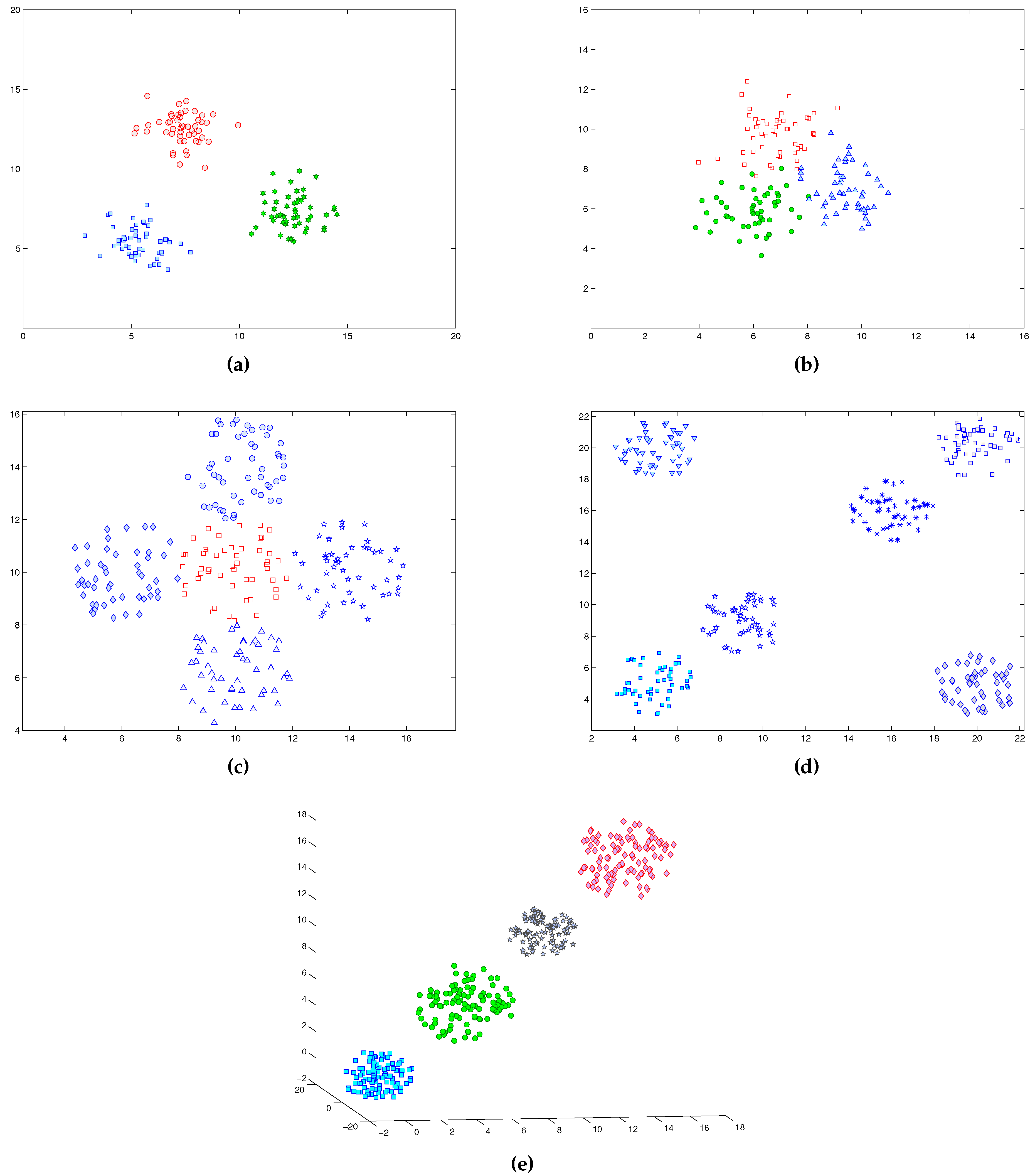
Figure 7.
Synthetic datasets used in comparison, (a) Separate 3, (b) Overlap 3, (c) Overlap 5, (d) Separate 6 and (e) Separate 4.
Figure 7.
Synthetic datasets used in comparison, (a) Separate 3, (b) Overlap 3, (c) Overlap 5, (d) Separate 6 and (e) Separate 4.

Figure 8.
Big datasets results.

Figure 9.
Cluster analysis for 3 datasets.

Figure 10.
Cluster analysis for 2 datasets.

Figure 11.
Cluster analysis for 2 big datasets.


Table 1.
Description of the datasets.
| Name | Points | Dimensions | Actual Clusters | Type (Synthetic/Real) |
|---|---|---|---|---|
| Overlap 3 | 150 | 2 | 3 | S |
| Separate 3 | 150 | 2 | 3 | S |
| Separate 4 | 400 | 2 | 4 | S |
| Overlap 5 | 250 | 2 | 5 | S |
| Separate 6 | 300 | 2 | 6 | S |
| Iris | 150 | 4 | 3 | R |
| Breast cancer | 683 | 9 | 2 | R |
Table 2.
Parameter Setting.
| Parameter | Definition | Value |
|---|---|---|
| Initial temperature | ||
| Final temperature | ||
| Cooling ratio | 0.9 | |
| M | Annealing epoch length | 8 |
| Max. number of clusters | ||
| Min. number of clusters | 2 | |
| Diversification parameter |
Table 3.
Performance of FCM, FVGA, MEPSO and KMC.
| Data Sets | Algorithm | Clusters | Misclass |
|---|---|---|---|
| Overlap 5 | KMC | 5.00 ± 0.00 | 12.70 ± 2.2965 |
| MEPSO | 5.05 ± 0.0931 | 5.25 ± 0.096 | |
| FVGA | 8.15 ± 0.0024 | 15.75 ± 0.154 | |
| FCM | NA | 19.50 ± 1.342 | |
| Separate 6 | KMC | 6.00 ± 0.00 | 0.00 ± 0.00 |
| MEPSO | 6.45 ± 0.0563 | 4.50 ± 0.023 | |
| FVGA | 6.95 ± 0.021 | 10.25 ± 0.373 | |
| FCM | NA | 26.50 ± 0.433 | |
| Separate 4 | KMC | 4.00 ± 0.00 | 0.00 ± 0.00 |
| MEPSO | 4.00 ± 0.00 | 1.50 ± 0.035 | |
| FVGA | 4.75 ± 0.0193 | 4.55 ± 0.05 | |
| FCM | NA | 8.95 ± 0.15 | |
| Breast cancer | KMC | 2.00 ± 0.00 | 34.65 ± 3.2971 |
| MEPSO | 2.05 ± 0.0563 | 25.00 ± 0.09 | |
| FVGA | 2.50 ± 0.0621 | 26.50 ± 0.80 | |
| FCM | NA | 30.23 ± 0.46 |
Table 4.
Performance of FCM, VGA and CCEA.
| Data sets | Algorithm | Clusters | Misclass |
|---|---|---|---|
| Separate 3 | KMC | 3.00 ± 0.00 | 0.00 ± 0.00 |
| CCEA | 3.00 ± 0.00 | 0.00 ± 0.00 | |
| VGA | 3.06 ± 0.07 | 0.34 ± 0.40 | |
| Overlap 3 | KMC | 3.00 ± 0.00 | 8.624 ± 0.41 |
| CCEA | 3.48 ± 0.21 | 16.22 ± 5.21 | |
| VGA | 4.22 ± 0.28 | 26.56 ± 5.11 | |
| Overlap 5 | KMC | 5.00 ± 0.00 | 12.68 ± 2.55 |
| CCEA | 5.00 ± 0.00 | 9.90 ± 0.62 | |
| VGA | 5.16 ± 0.13 | 16.82 ± 3.78 | |
| Separate 6 | KMC | 6.00 ± 0.00 | 0.00 ± 0.00 |
| CCEA | 6.00 ± 0.00 | 0.30 ± 0.13 | |
| VGA | 6.12 ± 0.11 | 3.08 ± 2.52 | |
| Iris | KMC | 2.00 ± 0.00 | 50.00 ± 0.00 |
| CCEA | 3.00 ± 0.00 | 27.96 ± 2.39 | |
| VGA | 3.00 ± 0.00 | 16.76 ± 0.12 |
Table 5.
Results of clustering in real world datasets with known classes.
| Name | Points | Dimensions | Actual Clusters | Computed Clusters |
|---|---|---|---|---|
| LiverDisorder | 345 | 6 | 2 | 2 |
| Heart | 297 | 13 | 2 | 2 |
| Sonar | 208 | 60 | 2 | 2 |
| Wine | 178 | 13 | 3 | 3 |
| Diabetes | 768 | 8 | 2 | 2 |
| Voting | 435 | 16 | 2 | 2 |
| Ionosphere | 351 | 34 | 2 | 2 |
| Bavaria1 | 89 | 3 | 2 | 2 |
| Bavaria2 | 89 | 4 | 2 | 2 |
| German_towns | 59 | 2 | 2 | 2 |
Table 6.
Datasets with big numbers of attributes.
| Name | Points | Dimensions | Actual Clusters | Computed Clusters |
|---|---|---|---|---|
| Hill-Valley | 606 | 100 | 2 | 2 |
| LSVT | 126 | 309 | 2 | 2 |
© 2018 by the authors. Licensee MDPI, Basel, Switzerland. This article is an open access article distributed under the terms and conditions of the Creative Commons Attribution (CC BY) license (http://creativecommons.org/licenses/by/4.0/).
Share and Cite
MDPI and ACS Style
Hedar, A.-R.; Ibrahim, A.-M.M.; Abdel-Hakim, A.E.; Sewisy, A.A. K-Means Cloning: Adaptive Spherical K-Means Clustering. Algorithms 2018, 11, 151. https://doi.org/10.3390/a11100151
AMA Style
Hedar A-R, Ibrahim A-MM, Abdel-Hakim AE, Sewisy AA. K-Means Cloning: Adaptive Spherical K-Means Clustering. Algorithms. 2018; 11(10):151. https://doi.org/10.3390/a11100151
Chicago/Turabian StyleHedar, Abdel-Rahman, Abdel-Monem M. Ibrahim, Alaa E. Abdel-Hakim, and Adel A. Sewisy. 2018. "K-Means Cloning: Adaptive Spherical K-Means Clustering" Algorithms 11, no. 10: 151. https://doi.org/10.3390/a11100151
Note that from the first issue of 2016, this journal uses article numbers instead of page numbers. See further details here.