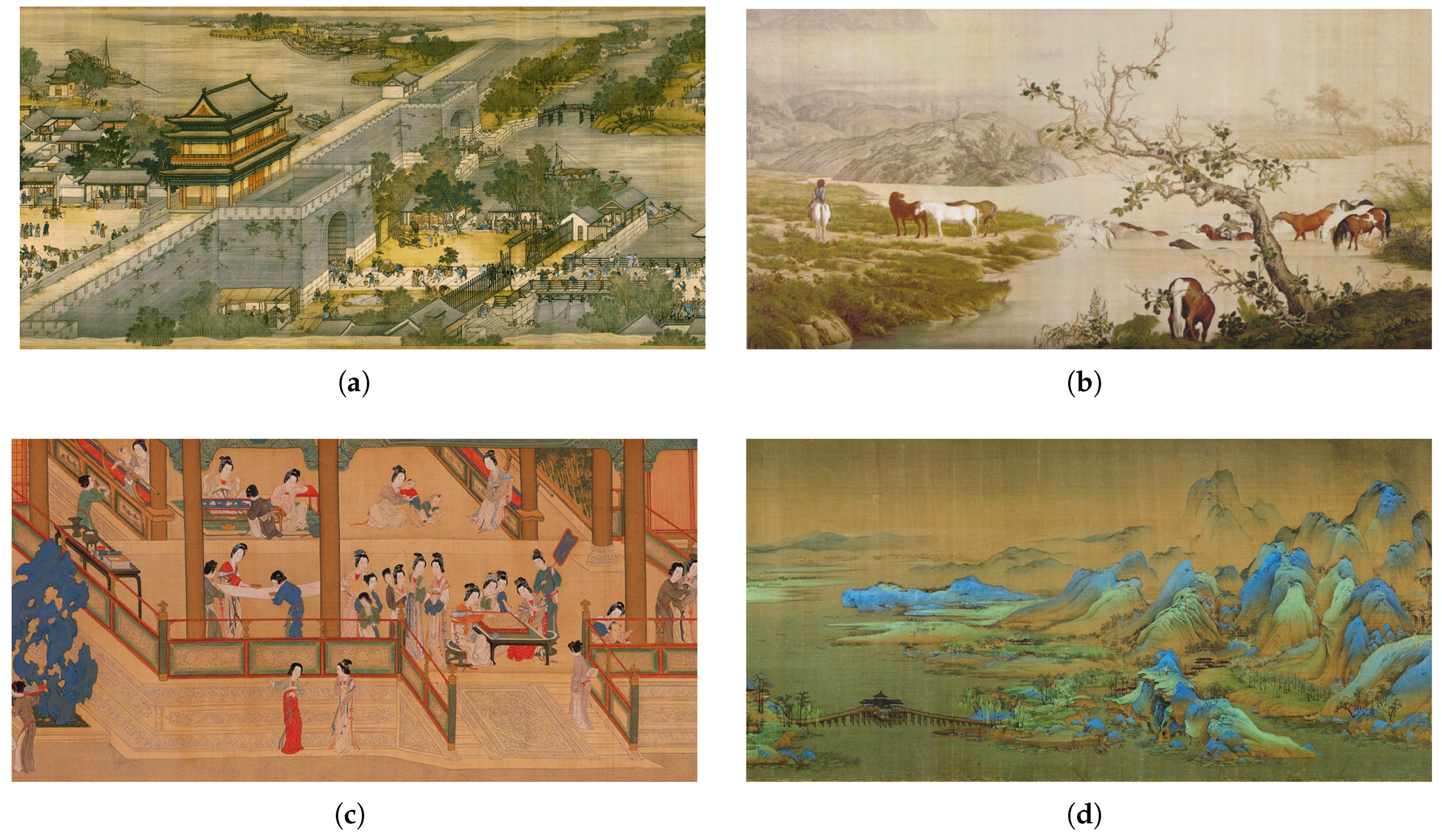
Figure 1.
(a) Part of Along the River during the Qingming Festival (original size: 38,414 × 1800); (b) part of One Hundred Horses (original size: 16,560 × 2022); (c) part of Spring Morning in the Han Palace (original size: 102,955 × 5228); (d) part of A Thousand Li of Rivers and Mountains (original size: 150,000 × 6004).
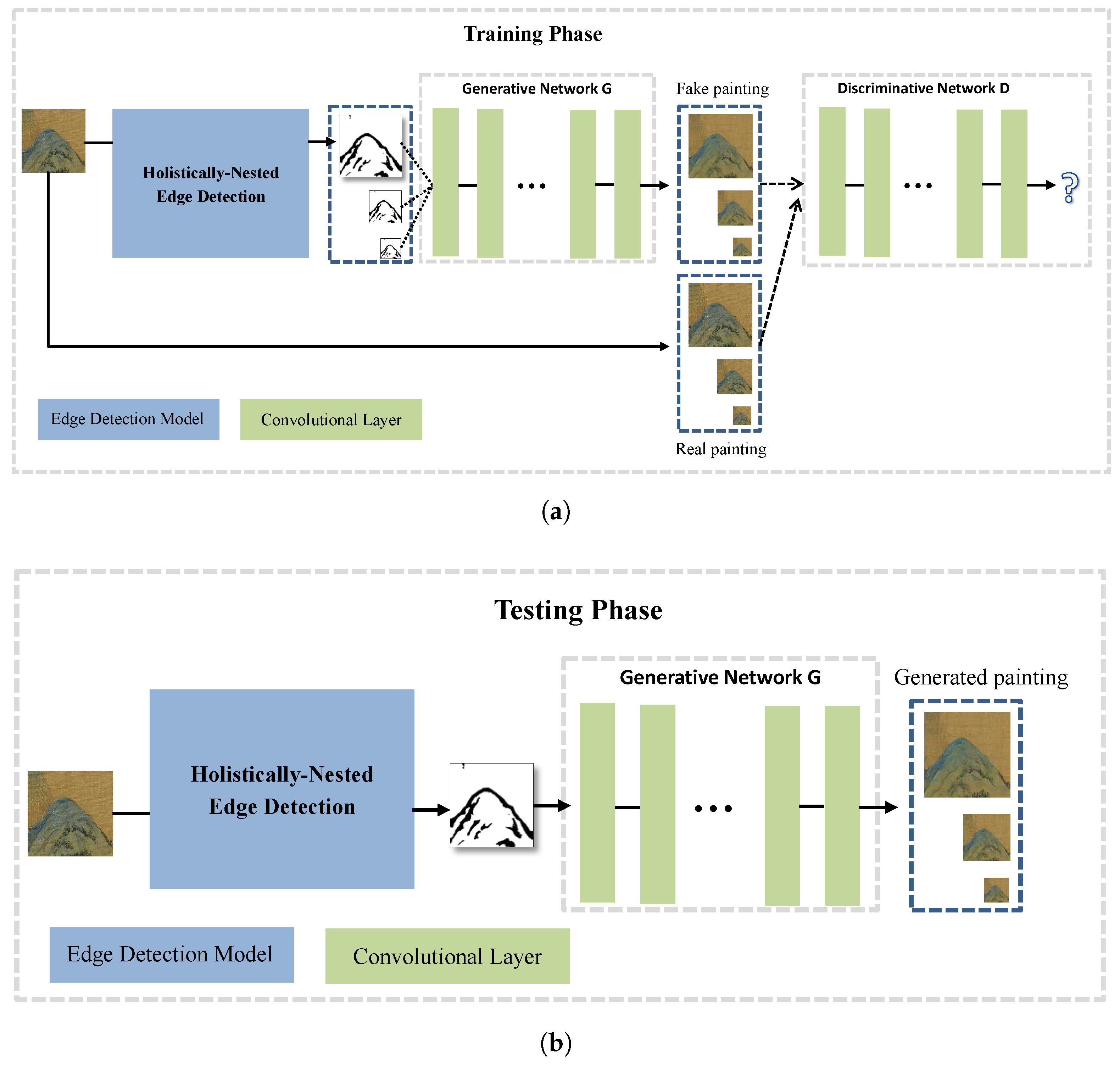
Figure 2.
Overview of the proposed approach. Training a multiscale deep neural network that can generate a Chinese painting from a sketch. We use an edge detection model to produce the input sketch. (a) By training, the discriminative network can make a distinction between the real and fake paintings, and the generative network aims at fooling the discriminative network by training; (b) after training, the generator can create realistic paintings.
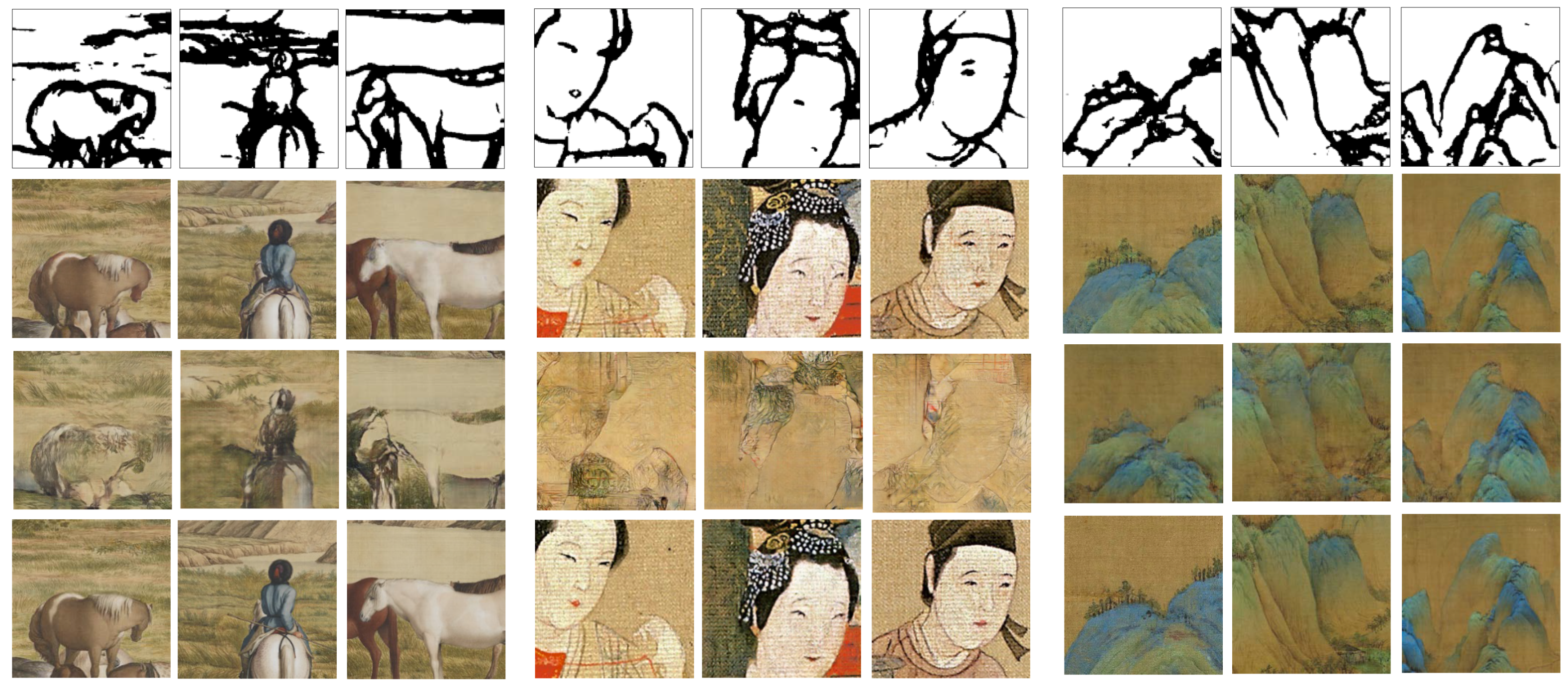
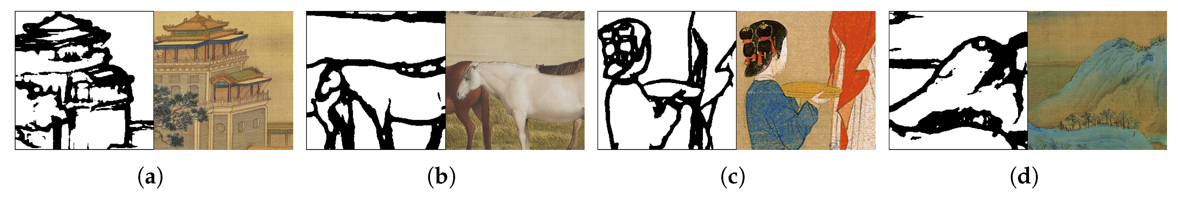
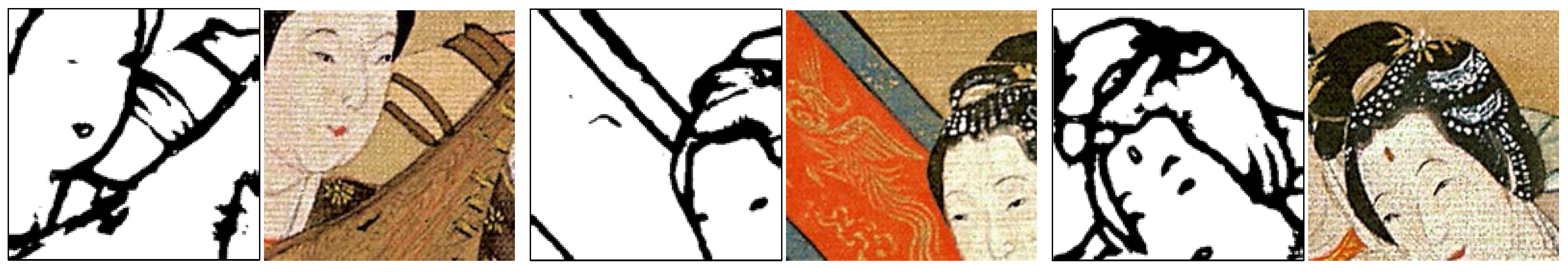
Figure 3.
Exemplary pairs from our training data, sketches (left) and paintings (right). (a) Along the River during the Qingming Festival; (b) One Hundred Horses; (c) Spring Morning in the Han Palace; (d) A Thousand Li of Rivers and Mountains.
Figure 3.
Exemplary pairs from our training data, sketches (left) and paintings (right). (a) Along the River during the Qingming Festival; (b) One Hundred Horses; (c) Spring Morning in the Han Palace; (d) A Thousand Li of Rivers and Mountains.
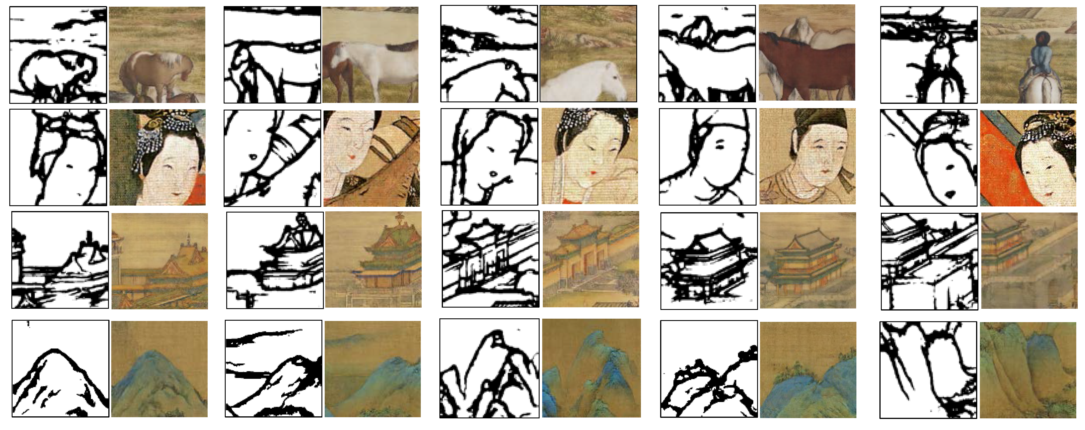
Figure 4.
Our deep network takes user sketches to synthesize Chinese paintings. The input sketch can be any size, and our deep network can synthesize the Chinese painting with fine details in real time. Despite the diverse sketch styles, our network can produce high quality and diverse results. (Left) Input sketch; (right) generated Chinese painting.
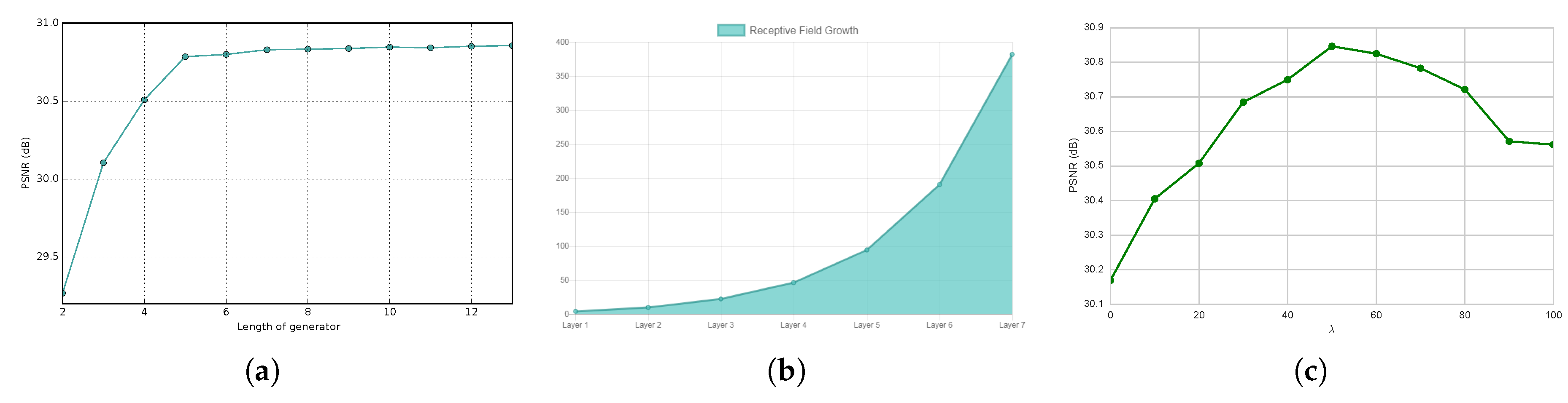
Figure 5.
(a) Length of the generator vs. the PSNR of generated testing painting; (b) length of the discriminator vs. the size of the recptive field; (c) vs. the PSNR of the generated testing painting.
Figure 5.
(a) Length of the generator vs. the PSNR of generated testing painting; (b) length of the discriminator vs. the size of the recptive field; (c) vs. the PSNR of the generated testing painting.
Figure 6.
Comparison of experimental results to Pix2pix. From top to bottom: input sketch, our deep network, Pix2pix and the ground truth.
Figure 6.
Comparison of experimental results to Pix2pix. From top to bottom: input sketch, our deep network, Pix2pix and the ground truth.
Figure 7.
Some facial images in the training data.
Figure 7.
Some facial images in the training data.
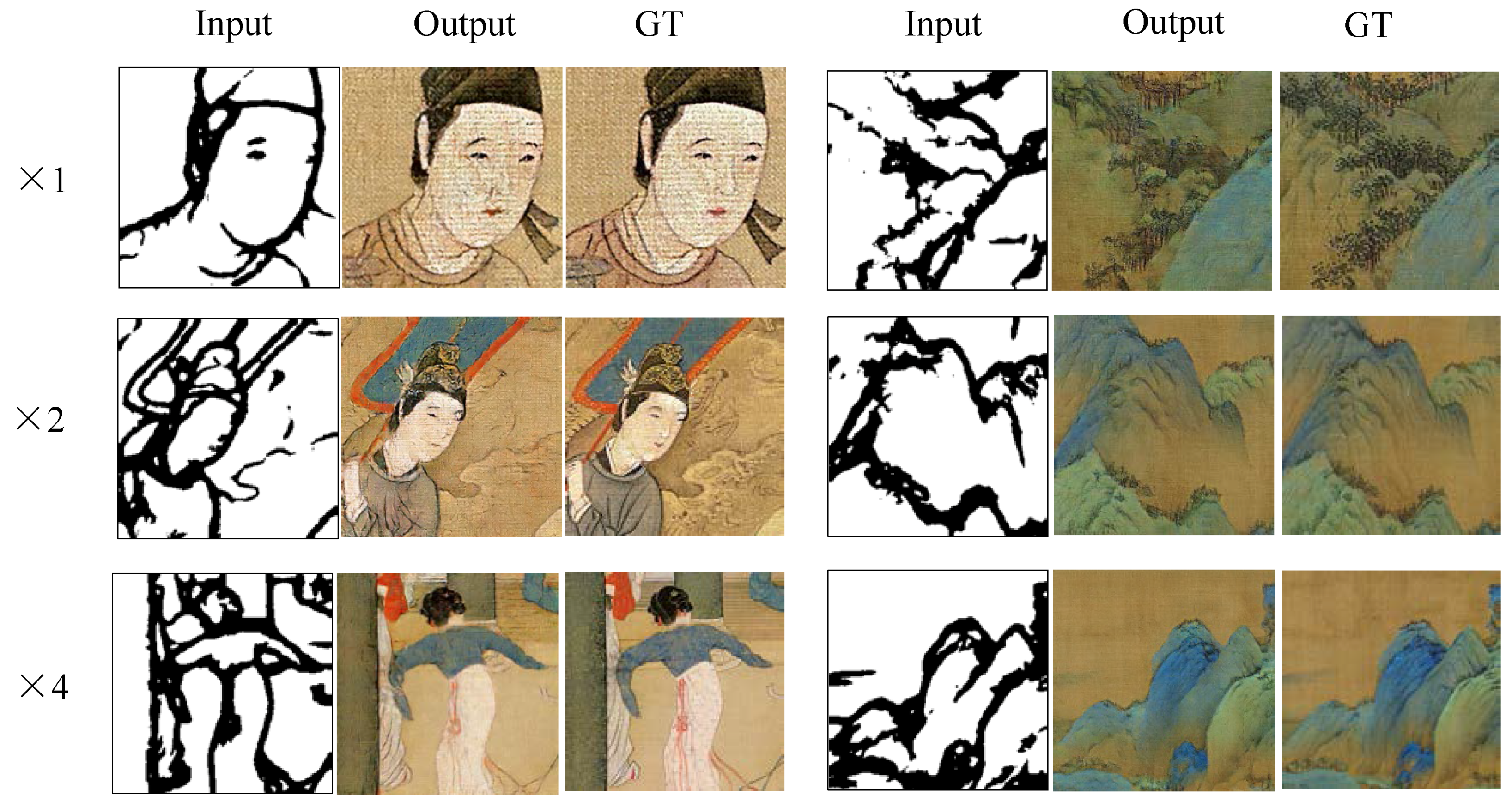
Figure 8.
Multi-scale input and its corresponding output. We reduce the original image to 1/2 and 1/4 of the original size by bilinear interpolation to generate multiscale images. (Top) The small level scale input sketch; (middle) the middle-level scale input sketch; (bottom) the large level scale input sketch.
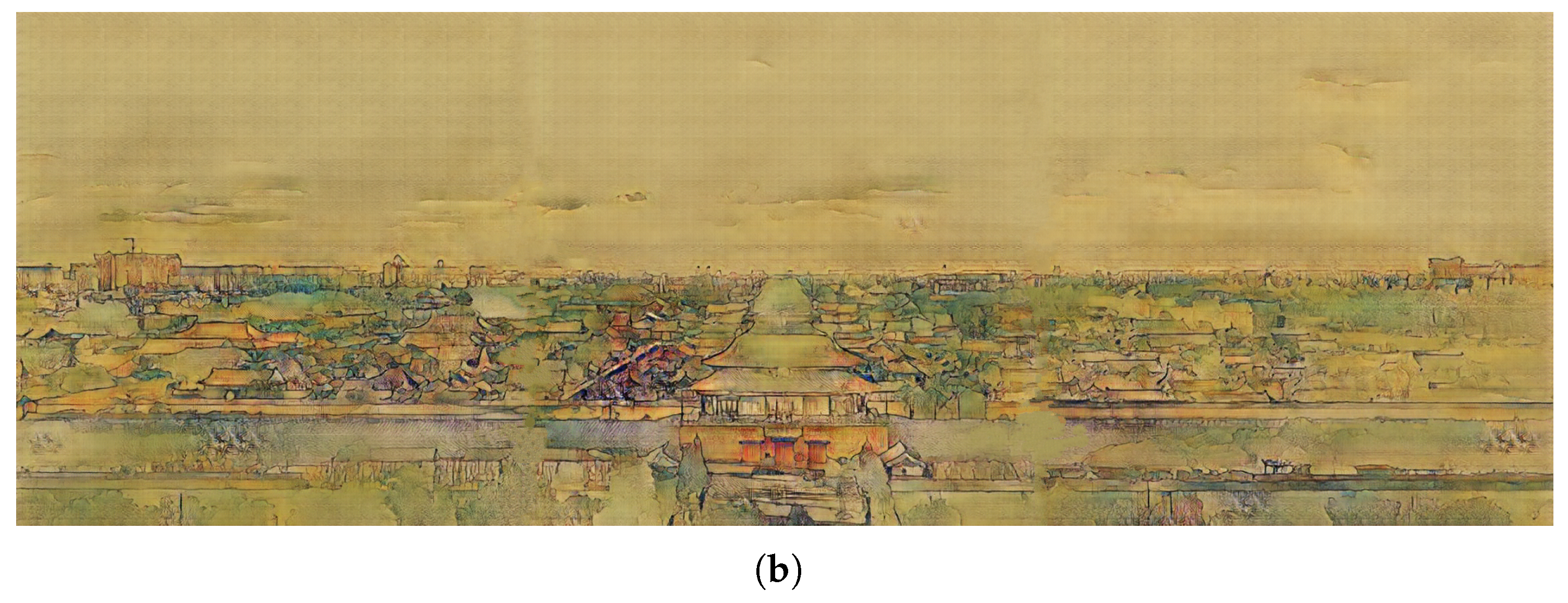
Figure 9.
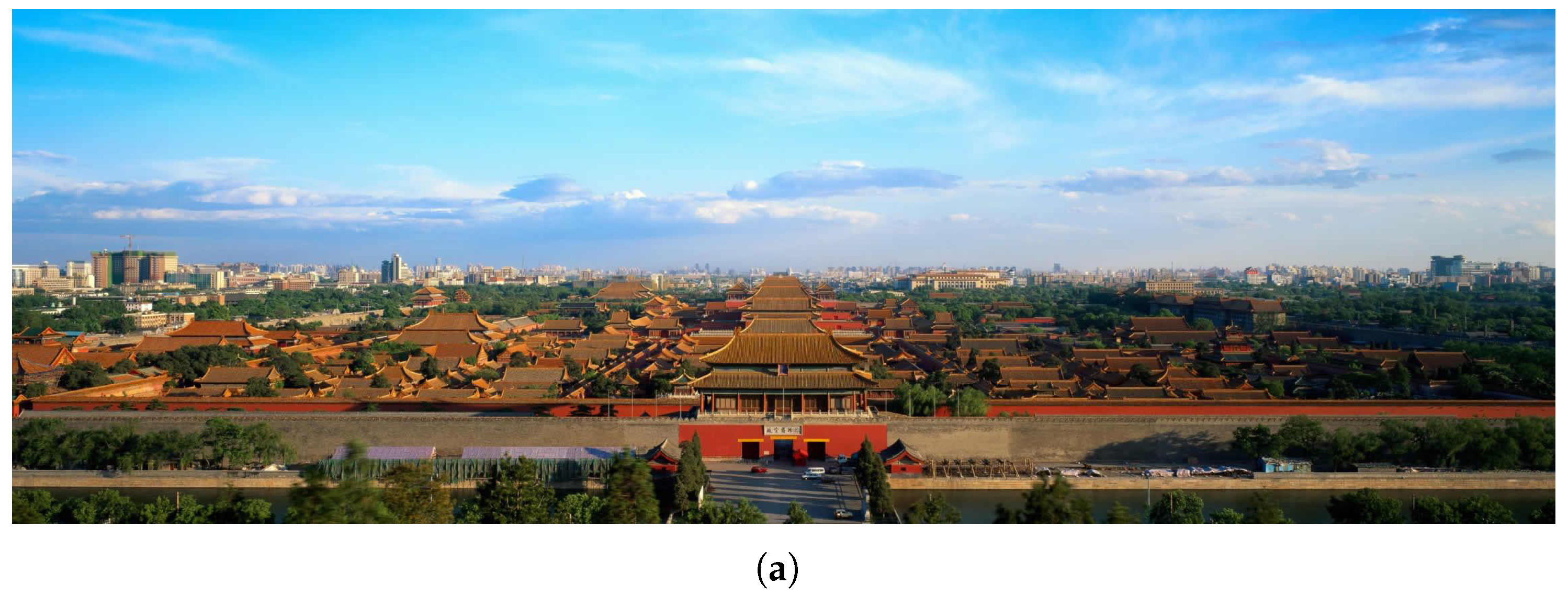
Transforming a real image into a Chinese painting. Our network can handle any size of images. (a) Input image; (b) Chinese painting produced by our network. The input image has an enormous size of (2300, 768); because of the graphics memory constraints, we divided this huge images into three parts to process.
Figure 9.
Transforming a real image into a Chinese painting. Our network can handle any size of images. (a) Input image; (b) Chinese painting produced by our network. The input image has an enormous size of (2300, 768); because of the graphics memory constraints, we divided this huge images into three parts to process.
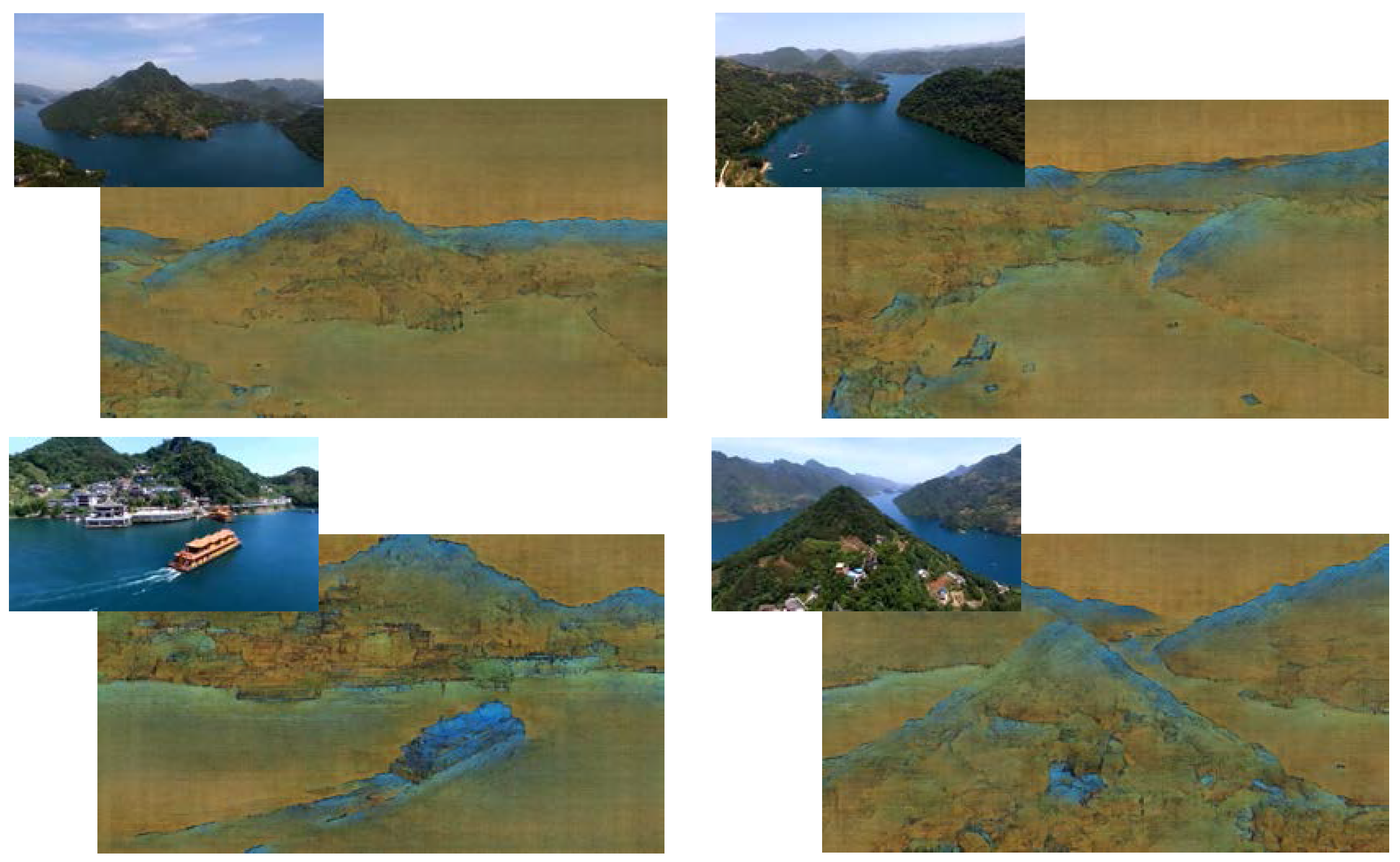
Figure 10.
Transforming an aerial photograph into the Chinese painting style video. For the whole video, please see the additional files.
Figure 10.
Transforming an aerial photograph into the Chinese painting style video. For the whole video, please see the additional files.
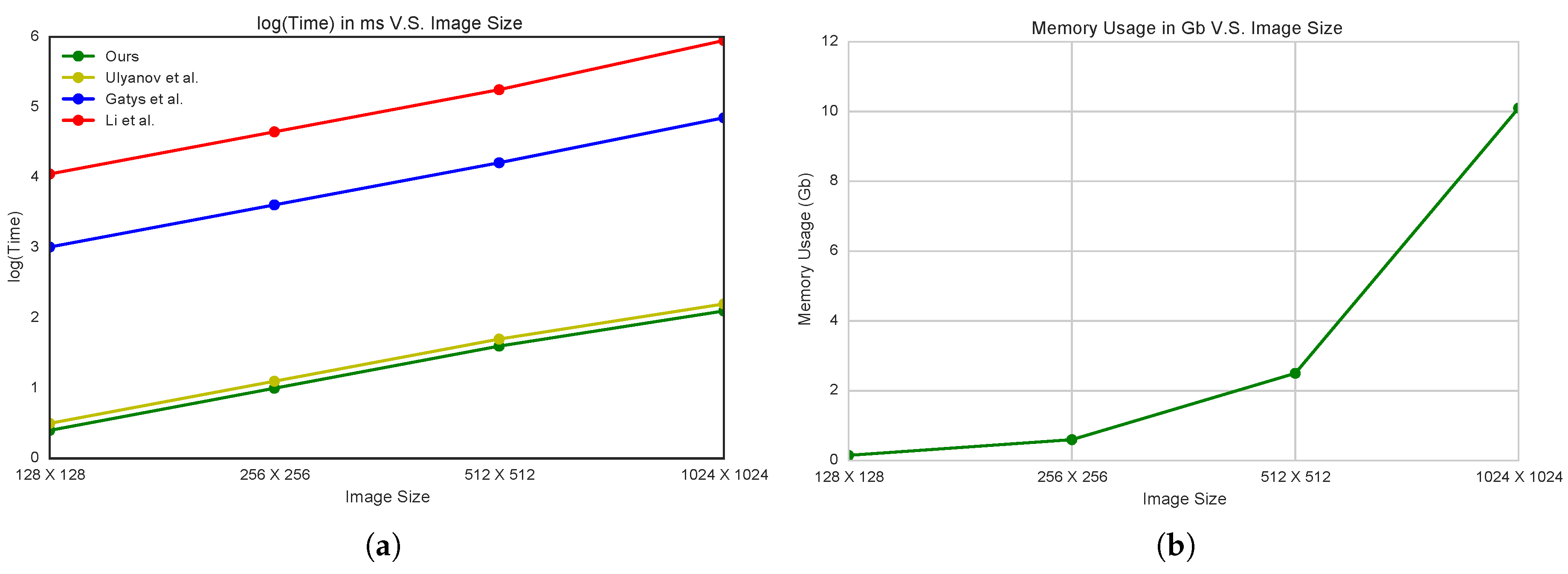
Figure 11.
(
a) Speed comparison (in log space) between our method and Gatys et al. [
2], Li et al. [
38] and Ulyanov et al. [
39]. The feed-forward methods (ours and Ulyanov et al. [
39]) are significantly faster than Gatys et al. [
2] (500-times speed up) and Li et al. [
38] (5000-times speed up). (
b) Memory usage vs. image size, the required memory is linearly related to the size of input image.
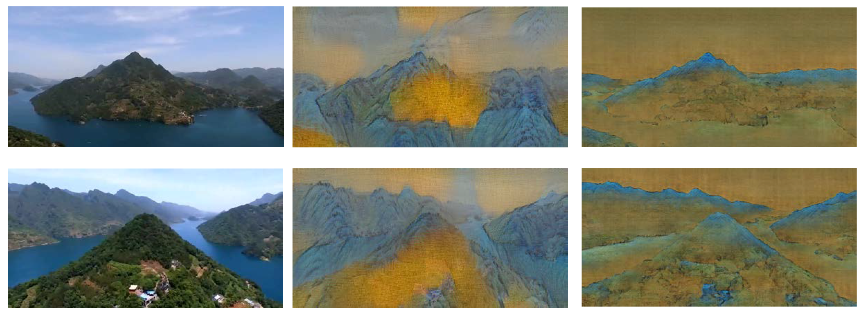
Figure 12.
Example results of style transfer using our image transformation networks. (left) Input image; (middle) results of Ulyanov et al. [
39]; (right) ours.
Figure 12.
Example results of style transfer using our image transformation networks. (left) Input image; (middle) results of Ulyanov et al. [
39]; (right) ours.
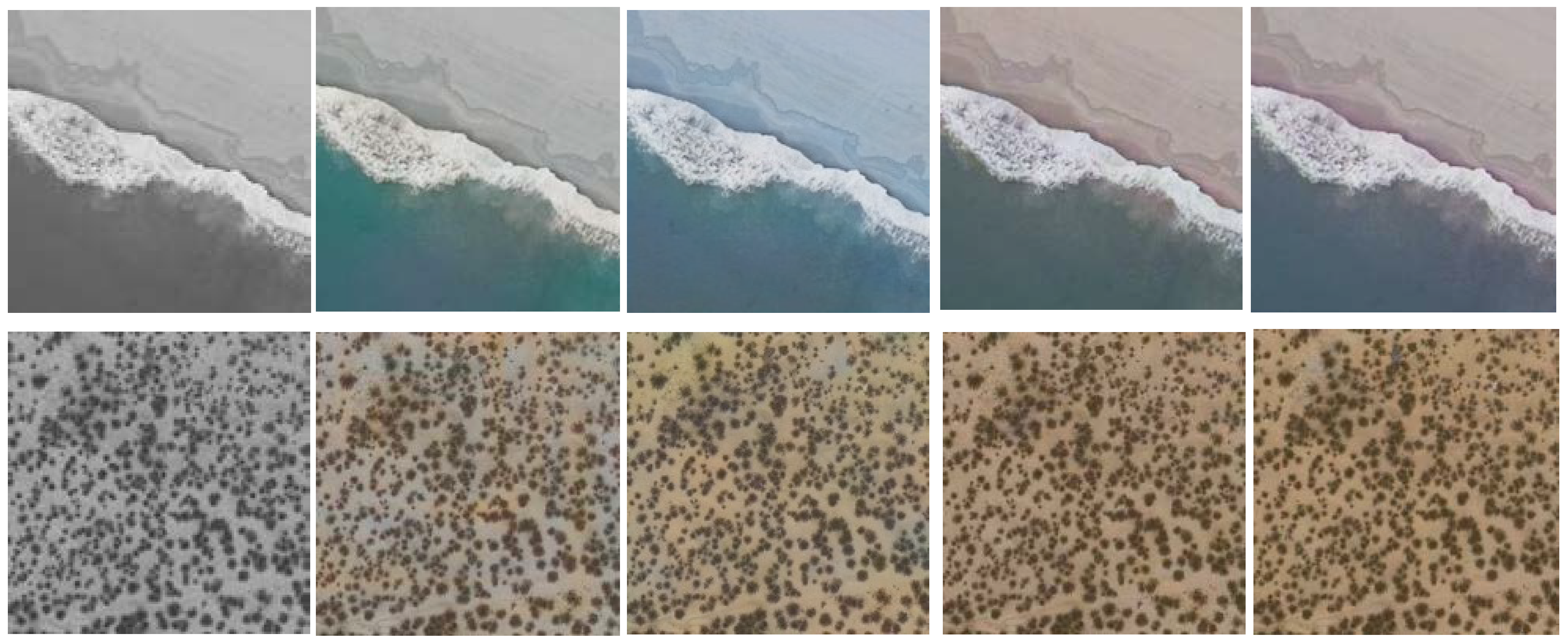
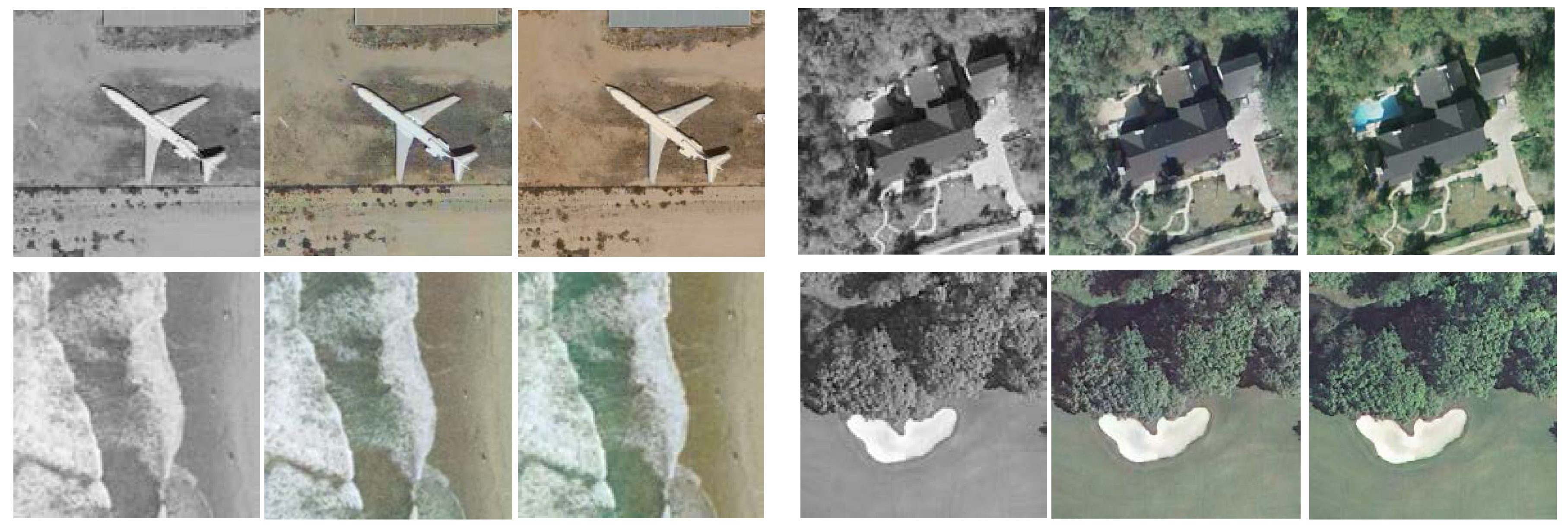
Figure 13.
Example artificial colorization of satellite images: grayscale images (left), colorful images (middle) and ground truth (right).
Figure 13.
Example artificial colorization of satellite images: grayscale images (left), colorful images (middle) and ground truth (right).
Figure 14.
We compare against the other methods. The first column contains the input image; the second column is the result of [
25]; the third column is the result of [
41]; the fourth column is our result; and the last row is the ground truth.
Figure 14.
We compare against the other methods. The first column contains the input image; the second column is the result of [
25]; the third column is the result of [
41]; the fourth column is our result; and the last row is the ground truth.
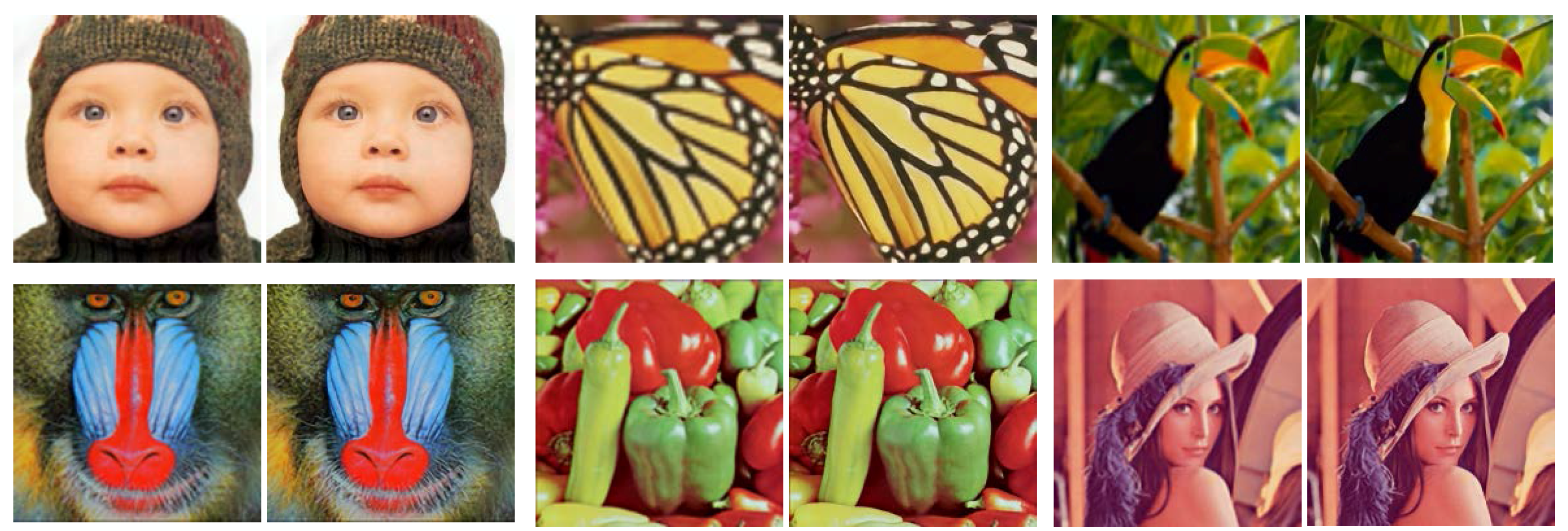
Figure 15.
Super-resolution results of images in Set5 [
47] and Set14 [
46]. Our method takes the bicubic interpolation of low-resolution images (
left) as input and high-resolution images (
right,
) as output.
Figure 15.
Super-resolution results of images in Set5 [
47] and Set14 [
46]. Our method takes the bicubic interpolation of low-resolution images (
left) as input and high-resolution images (
right,
) as output.
Figure 16.
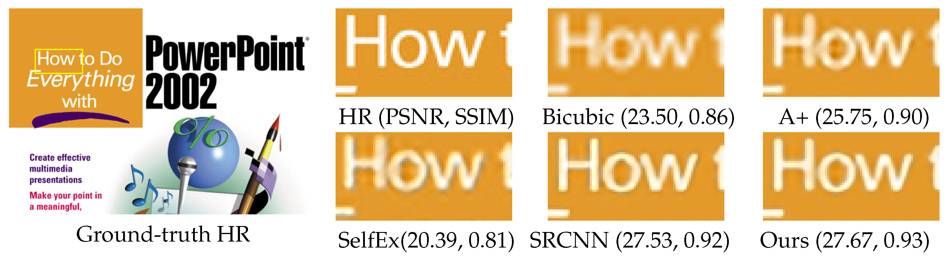
Image “ppt3” (Set14, ): there are sharper edges between “H”, “o” and “w” in our result; while in other works, the text is blurry. SR, Super-Resolution.
Figure 16.
Image “ppt3” (Set14, ): there are sharper edges between “H”, “o” and “w” in our result; while in other works, the text is blurry. SR, Super-Resolution.
Table 1.
Generative model network architectures. Conv means convolutional layer; BN means batch normalization; ReLU means rectified linear unit.
Table 1.
Generative model network architectures. Conv means convolutional layer; BN means batch normalization; ReLU means rectified linear unit.
| Generative Model |
|---|
| Name | Kernel Size | Stride | Pad | Norm | Activation |
|---|
| Conv1 | 3 × 3 × 3 × 64 | 1 | 1 | - | ReLU |
| Conv2 | 3 × 3 × 64 × 64 | 1 | 1 | BN | ReLU |
| Conv3 | 3 × 3 × 64 × 64 | 1 | 1 | BN | ReLU |
| Conv4 | 3 × 3 × 64 × 64 | 1 | 1 | BN | ReLU |
| Conv5 | 3 × 3 × 64 × 64 | 1 | 1 | BN | ReLU |
| Conv6 | 3 × 3 × 64 × 64 | 1 | 1 | BN | ReLU |
| Conv7 | 3 × 3 × 64 × 64 | 1 | 1 | BN | ReLU |
| Conv8 | 3 × 3 × 64 × 64 | 1 | 1 | BN | ReLU |
| Conv9 | 3 × 3 × 64 × 64 | 1 | 1 | BN | ReLU |
| Conv10 | 3 × 3 × 64 × 3 | 1 | 1 | - | ReLU |
Table 2.
Discriminative model network architectures. Conv means Convolutional layer; BN means Batch Normalization; Leaky means leaky rectified linear unit.
Table 2.
Discriminative model network architectures. Conv means Convolutional layer; BN means Batch Normalization; Leaky means leaky rectified linear unit.
| Discriminative Model |
|---|
| Name | Kernel Size | Stride | Pad | Norm | Activation |
|---|
| Conv1 | 4 × 4 × 3 × 64 | 2 | 1 | - | Leaky |
| Conv2 | 4 × 4 × 64 × 128 | 2 | 1 | BN | Leaky |
| Conv3 | 4 × 4 × 128 × 256 | 2 | 1 | BN | Leaky |
| Conv4 | 4 × 4 × 256 × 512 | 2 | 1 | BN | Leaky |
| Conv5 | 4 × 4 × 512 × 512 | 2 | 1 | BN | Leaky |
| Conv6 | 4 × 4 × 512 × 512 | 2 | 1 | BN | Leaky |
| Conv7 | 4 × 4 × 512 × 1 | 2 | 1 | BN | - |
Table 3.
We evaluate the trade-off between performance and speed in networks with different depths.
Table 3.
We evaluate the trade-off between performance and speed in networks with different depths.
| Length of Generator | 7 | 8 | 9 | 10 | 11 | 12 | 13 |
|---|
| PSNR (dB) | 30.829 | 30.832 | 30.837 | 30.846 | 30.842 | 30.852 | 30.856 |
| Times () | 0.023 s | 0.027 s | 0.029 s | 0.032 s | 0.035 s | 0.039 s | 0.044 s |
Table 4.
Quantitative evaluation of Pix2pix and our work. We evaluated average PSNR/SSIM for images in
Figure 6.
Table 4.
Quantitative evaluation of Pix2pix and our work. We evaluated average PSNR/SSIM for images in
Figure 6.
| | Images | Column 1 to 3 | Column 4–6 | Column 7–9 |
|---|
| Methods | |
|---|
| Pix2Pix (PSNR/SSIM) | 28.38/0.4534 | 28.08/0.3421 | 28.85/0.5312 |
| Ours (PSNR/SSIM) | 30.95/0.7282 | 28.76/0.5854 | 31.84/0.6863 |
Table 5.
Speed (in seconds) for our style transfer network vs. the optimization-based baseline for varying numbers of iterations and image resolutions. Both methods are benchmarked on a GTX 1080 GPU.
Table 5.
Speed (in seconds) for our style transfer network vs. the optimization-based baseline for varying numbers of iterations and image resolutions. Both methods are benchmarked on a GTX 1080 GPU.
| | Methods | Gatys et al. [2] | Ulyanov et al. [39] | Ours |
|---|
| Image Size | |
|---|
| 1.542 s | 0.004 s | 0.002 s |
| 6.483 s | 0.015 s | 0.008 s |
| 25.23 s | 0.051 s | 0.032 s |
| 106.2 s | 0.212 s | 0.122 s |
Table 6.
Results of our user study evaluating the naturalness of the colorizations.
Table 6.
Results of our user study evaluating the naturalness of the colorizations.
| Approach | Iizuka et al. [25] | Zhang et al. [41] | Ours | Ground Truth |
|---|
| Naturalness | 78.20% | 80.80% | 93.80% | 96.6% |
Table 7.
Quantitative evaluation of state-of-the-art SR methods. We evaluated average PSNR/SSIM for scale factors , and on datasets Set5, Set14.
Table 7.
Quantitative evaluation of state-of-the-art SR methods. We evaluated average PSNR/SSIM for scale factors , and on datasets Set5, Set14.
| Dataset | Scale | Bicubic | A+ | SelfEx | SRCNN | Ours |
|---|
| PSNR/SSIM | PSNR/SSIM | PSNR/SSIM | PSNR/SSIM | PSNR/SSIM |
|---|
| Set5 | ×2 | 33.66/0.9299 | 36.54/0.9544 | 36.54/0.9537 | 36.49/0.9537 | 36.66/0.9542 |
| ×3 | 30.39/0.8682 | 32.58/0.9088 | 32.43/0.9057 | 32.58/0.9093 | 32.75/0.9090 |
| ×4 | 28.42/0.8104 | 30.28/0.8603 | 30.14/0.8548 | 30.31/0.8619 | 30.48/0.8628 |
| Set14 | ×2 | 30.24/0.8688 | 32.28/0.9056 | 32.26/0.9040 | 32.22/0.9034 | 32.42/0.9063 |
| ×3 | 27.55/0.7742 | 29.13/0.8188 | 29.05/0.8164 | 29.16/0.8196 | 29.28/0.8209 |
| ×4 | 26.00/0.7027 | 27.32/0.7491 | 27.24/0.7451 | 27.40/0.7518 | 27.49/0.7503 |


