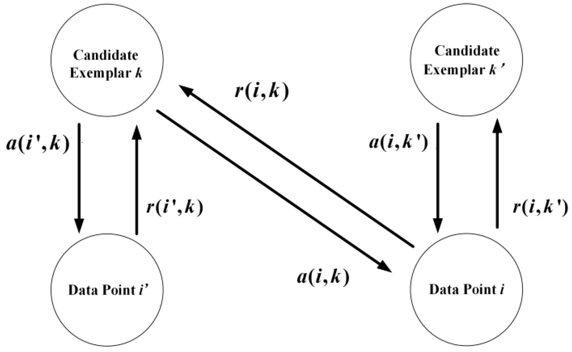
Figure 1.
Two messages, responsibility (, , and ), and availability (, , and ), are passing in an affinity propagation network. The responsibility and reflect how well the point acts as an exemplar to the point and , respectively. The availability and reflect how well the point and belong to a class centered on point . The responsibility reflects how well the point acts as an exemplar to the point . The availability reflects how well the point belongs to a class centered on point .
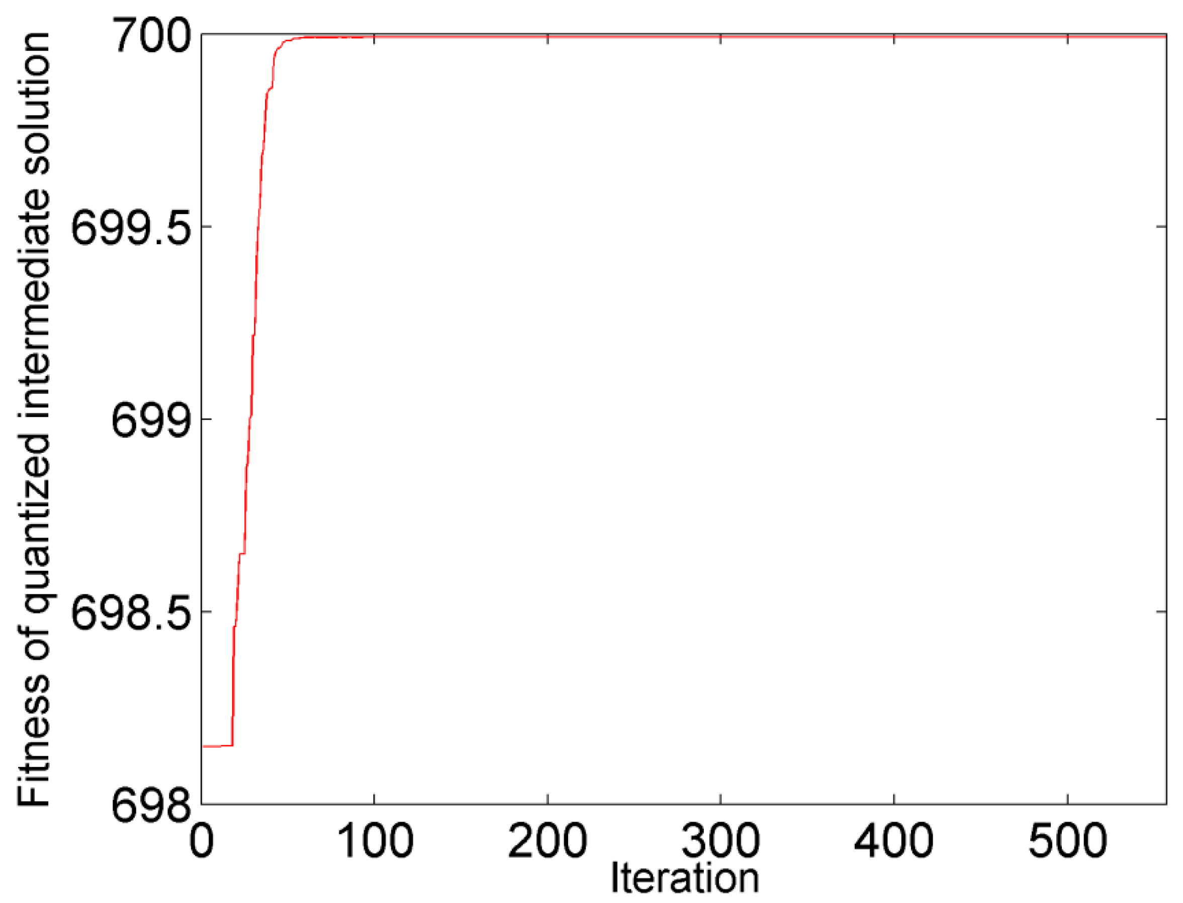
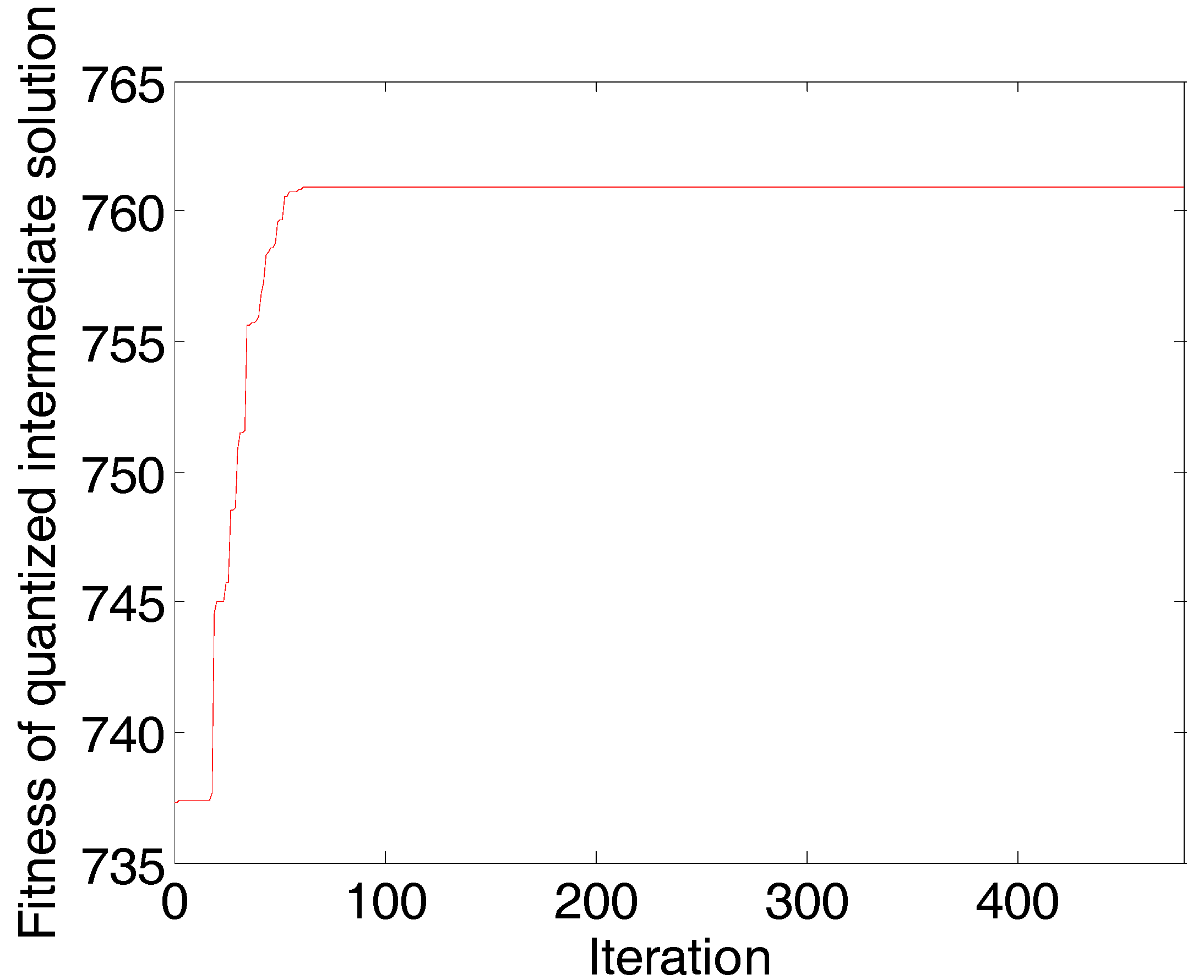
Figure 2.
The convergence diagram of the affinity propagation (AP) algorithm (corn data) in the first round: Iterations vs. Fitness (net similarity) of quantized intermediate solutions. When the iteration is 562, the network is converged.
Figure 2.
The convergence diagram of the affinity propagation (AP) algorithm (corn data) in the first round: Iterations vs. Fitness (net similarity) of quantized intermediate solutions. When the iteration is 562, the network is converged.
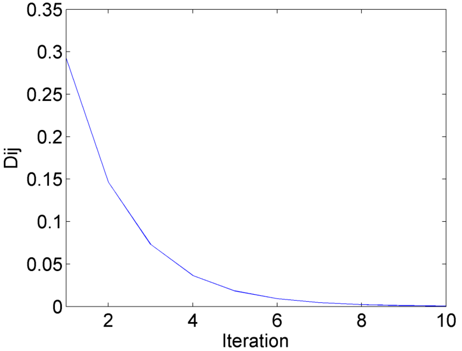
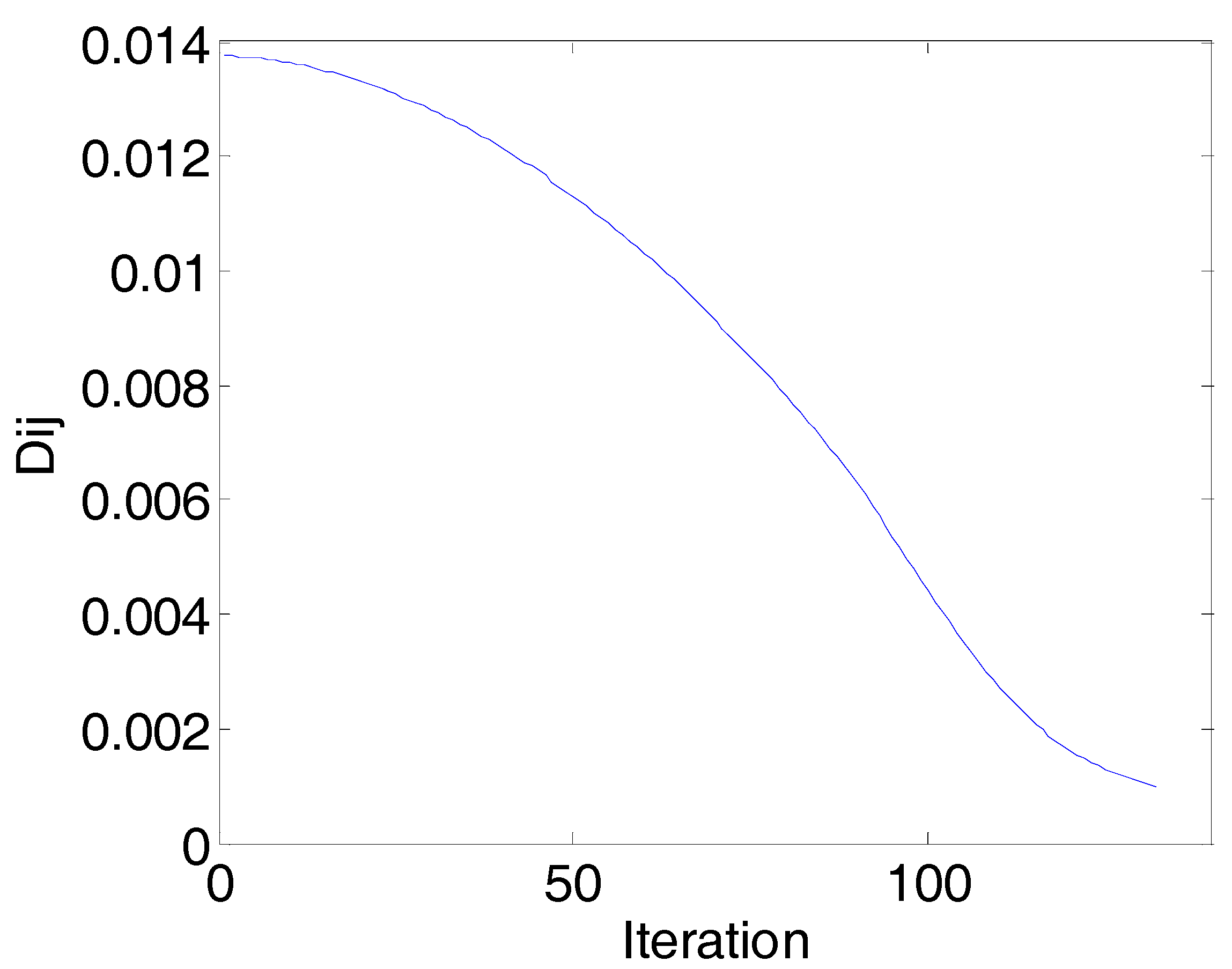
Figure 3.
The convergence diagram of the physarum network (PN) algorithm (corn data) in the first round: Iterations vs. (Dij is the rate of change of the network continuity). When the iteration is 10, all the Dij are smaller than the threshold of stop, and the network converges.
Figure 3.
The convergence diagram of the physarum network (PN) algorithm (corn data) in the first round: Iterations vs. (Dij is the rate of change of the network continuity). When the iteration is 10, all the Dij are smaller than the threshold of stop, and the network converges.
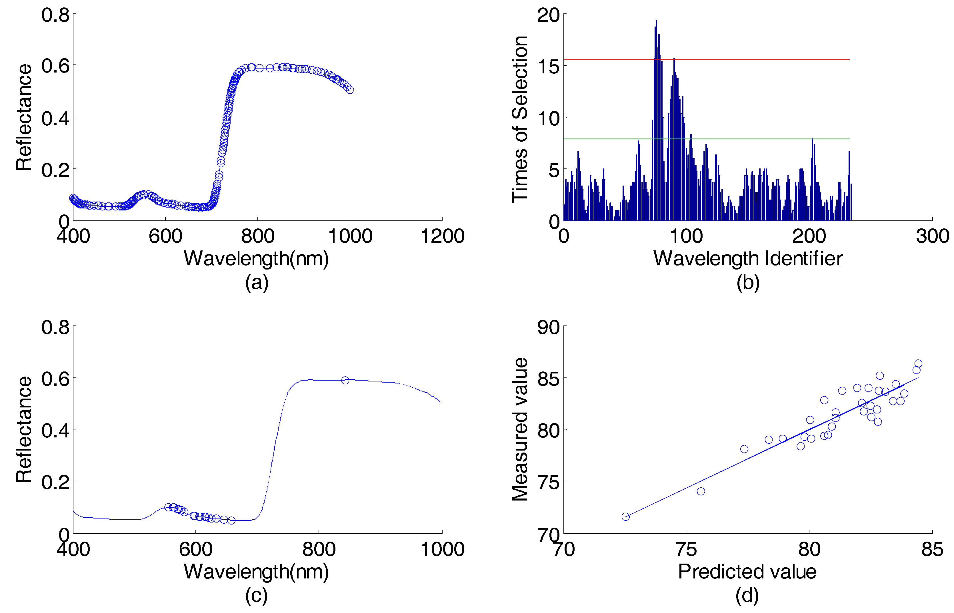
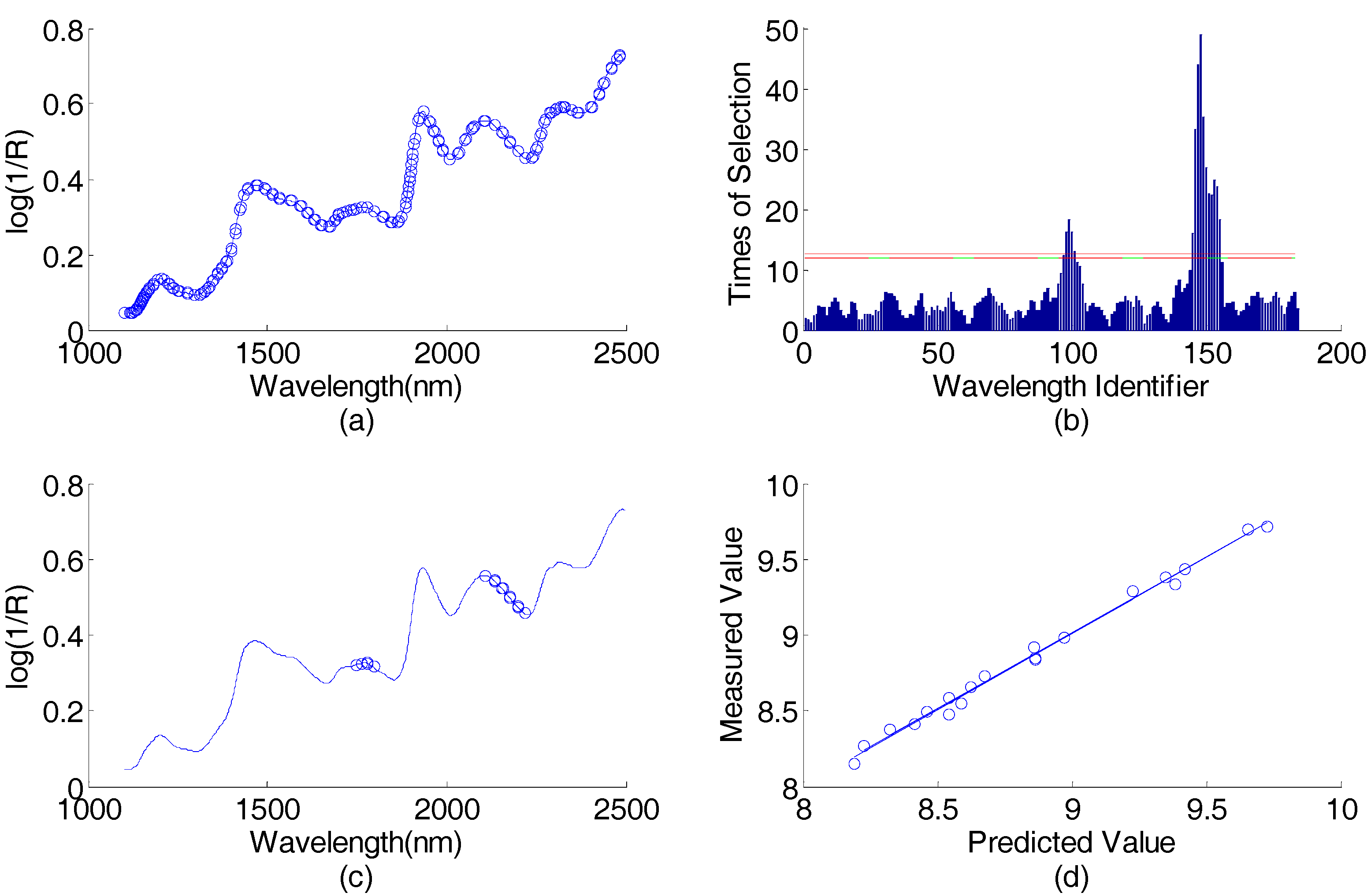
Figure 4.
Corn data (predicting protein content) wavelength selection result by using AP-PN-GA-PLS in the first round: (a) spectral responses vs. wavelengths, the 184 wavelengths selected by AP-PN are marked with circles; (b) times of selection (by GA-PLS) vs. wavelength identifier (1–184), the wavelengths above the lower line were selected; (c) spectral response vs. wavelengths, the 16 wavelengths selected by AP-PN-GA-PLS are marked with circles; (d) scatter plot of predicted values vs. the measured values. PLS = partial least square; GA = genetic algorithm.
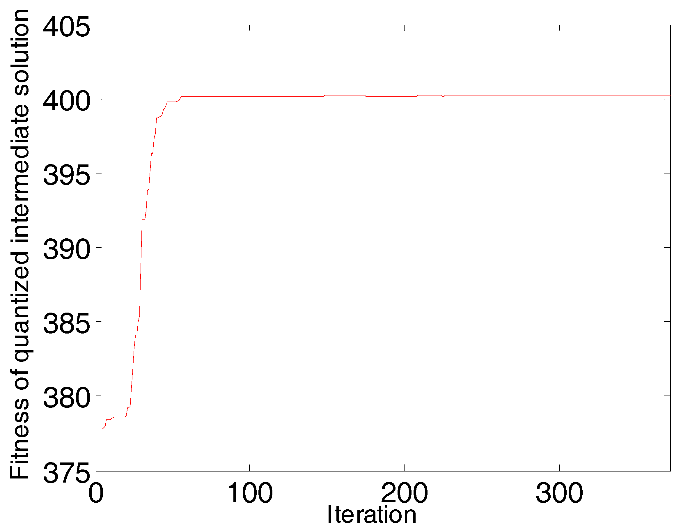
Figure 5.
The convergence diagram of the AP algorithm (diesel data): Iterations vs. Fitness (net similarity) of quantized intermediate solution in the first round. When the iteration is 386, the network is converged.
Figure 5.
The convergence diagram of the AP algorithm (diesel data): Iterations vs. Fitness (net similarity) of quantized intermediate solution in the first round. When the iteration is 386, the network is converged.
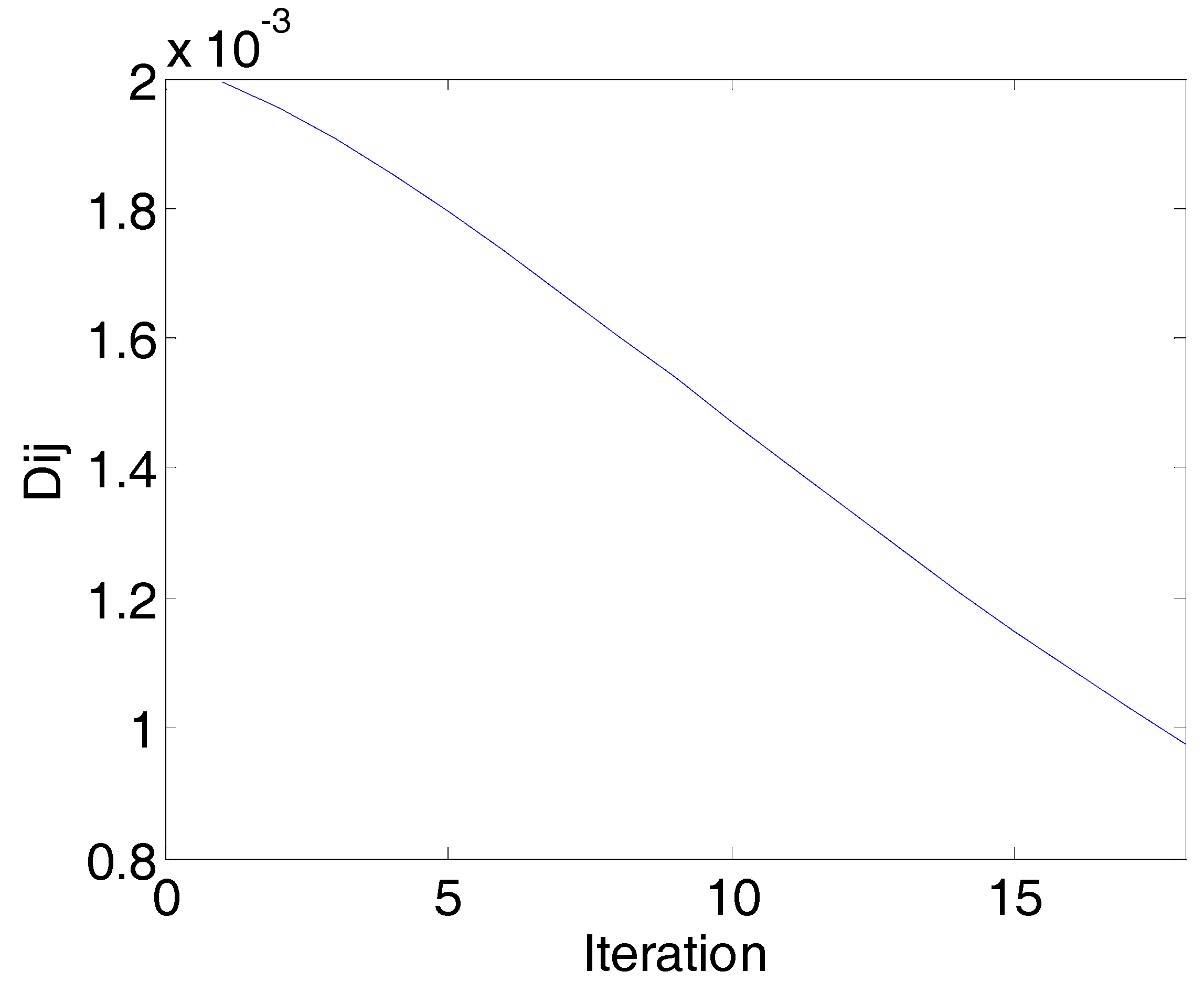
Figure 6.
The convergence diagram of the PN algorithm (corn data): Iterations vs. (Dij is the rate of change of the network continuity). When the iteration is 18, all the Dij are smaller than the threshold of stop, and the network is converged.
Figure 6.
The convergence diagram of the PN algorithm (corn data): Iterations vs. (Dij is the rate of change of the network continuity). When the iteration is 18, all the Dij are smaller than the threshold of stop, and the network is converged.
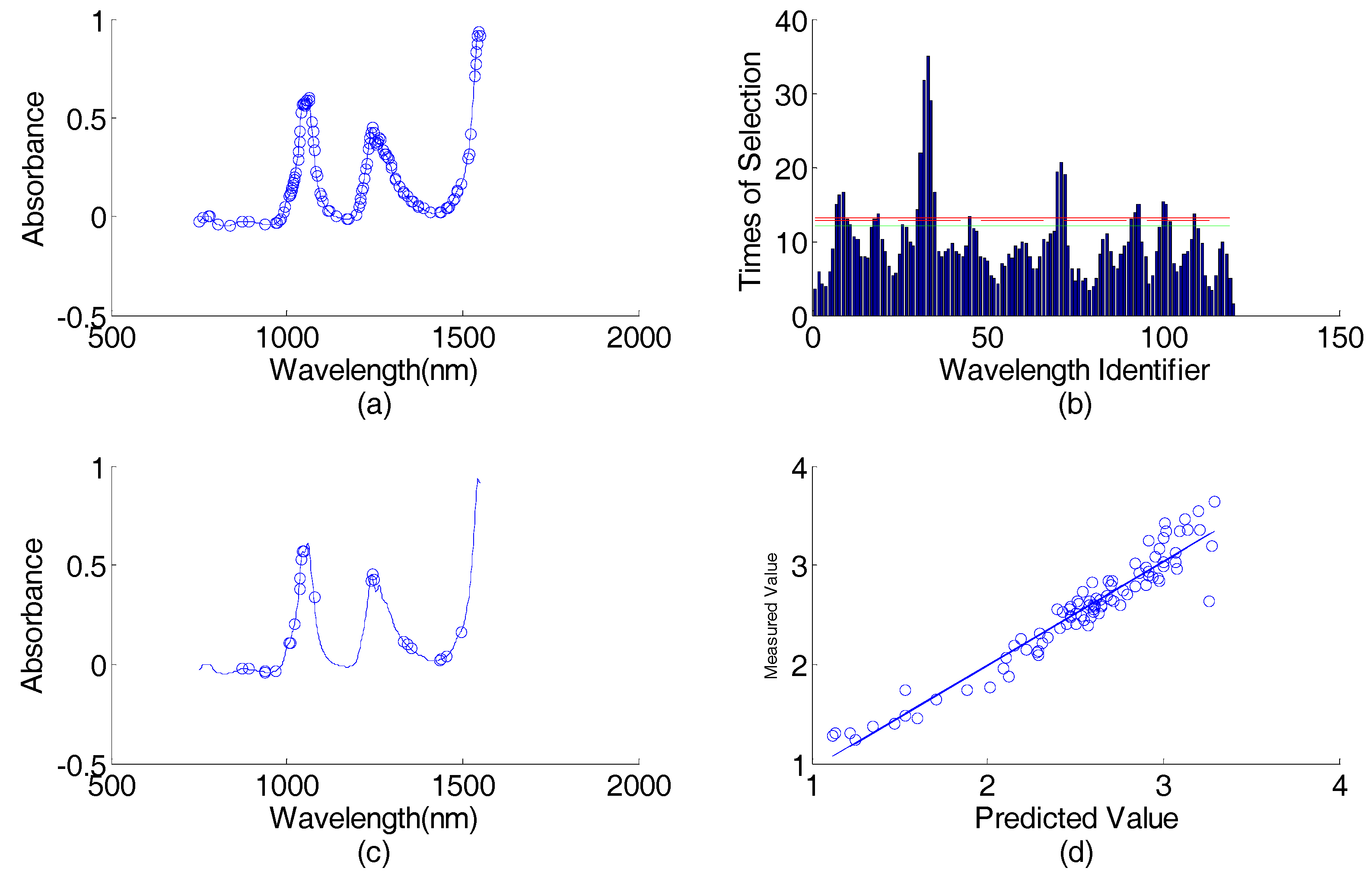
Figure 7.
Diesel data (predicting viscosity content) wavelength selection result in the first round: (a) spectral responses vs. wavelengths, the 120 wavelengths selected by AP-PN are marked with circles; (b) times of selection (by GA-PLS) vs. wavelength identifier (1–120); (c) spectral response vs. wavelengths, the 25 wavelengths selected by AP-PN-GA-PLS are marked with circles; (d) scatter plot of predicted values vs. the measured values.
Figure 8.
The convergence diagram of the AP algorithm (sweet orange leaves data) in the first round: Iterations vs. Fitness (net similarity) of quantized intermediate solutions. When the iteration is 486, the network is converged.
Figure 8.
The convergence diagram of the AP algorithm (sweet orange leaves data) in the first round: Iterations vs. Fitness (net similarity) of quantized intermediate solutions. When the iteration is 486, the network is converged.
Figure 9.
The convergence diagram of the PN algorithm (corn data) in the first round: Iterations vs. (Dij is the rate of change of the network continuity). When the iteration is 132, all the Dij are smaller than the threshold of stop, and the network is converged.
Figure 9.
The convergence diagram of the PN algorithm (corn data) in the first round: Iterations vs. (Dij is the rate of change of the network continuity). When the iteration is 132, all the Dij are smaller than the threshold of stop, and the network is converged.
Figure 10.
Sweet orange leaves data (predicting viscosity content) wavelength selection results in the first round: (a) spectral responses vs. wavelengths, the 234 wavelengths selected by AP-PN are marked with circles; (b) times of selection (by GA-PLS) vs. wavelength identifier (1–234); (c) spectral response vs. wavelengths, the 25 wavelengths selected by AP-PN-GA-PLS are marked with circles; (d) scatter plot of predicted values vs. the measured values.
Table 1.
The relationship between and the number of groups (corn data).
Table 1.
The relationship between and the number of groups (corn data).
| 0.5 | 0.6 | 0.7 | 0.8 | 0.9 |
| Number of groups | 184 | 184 | 184 | 184 | 184 |
Table 2.
The relationship between and the number of groups (diesel data).
Table 2.
The relationship between and the number of groups (diesel data).
| 0.5 | 0.6 | 0.7 | 0.8 | 0.9 |
| Number of groups | 120 | 120 | 120 | 120 | 120 |
Table 3.
The relationship between and the number of groups (orange leaves data).
Table 3.
The relationship between and the number of groups (orange leaves data).
| 0.5 | 0.6 | 0.7 | 0.8 | 0.9 |
| Number of groups | 234 | 234 | 234 | 234 | 234 |
Table 4.
The average values of the number of selected wavelengths, correlation coefficient (R), and predicted root mean square error (RMSEP) using PLS, GA-PLS, PN-GA-PLS, AP-GA-PLS, and AP-PN-GA-PLS (corn data).
Table 4.
The average values of the number of selected wavelengths, correlation coefficient (R), and predicted root mean square error (RMSEP) using PLS, GA-PLS, PN-GA-PLS, AP-GA-PLS, and AP-PN-GA-PLS (corn data).
| Method | Number of Input Wavelengths | Number of Selected Wavelengths | R | RMSEP(%) |
|---|
| PLS | 700 | 700 | 0.9832 | 0.0902 |
| GA-PLS | 700 | 67 | 0.9989 | 0.0431 |
| PN-GA-PLS | 700 | 35 | 0.9960 | 0.0597 |
| AP-GA-PLS | 700 | 39 | 0.9941 | 0.0643 |
| AP-PN-GA-PLS | 700 | 25 | 0.9970 | 0.0397 |
Table 5.
The average values of the number of selected wavelengths, R, and RMSEP using PLS, GA-PLS, PN-GA-PLS, AP-GA-PLS, and AP-PN-GA-PLS (diesel data).
Table 5.
The average values of the number of selected wavelengths, R, and RMSEP using PLS, GA-PLS, PN-GA-PLS, AP-GA-PLS, and AP-PN-GA-PLS (diesel data).
| Method | Number of Input Wavelengths | Number of Selected Wavelengths | R | RMSEP(%) |
|---|
| PLS | 401 | 401 | 0.9716 | 0.1370 |
| GA-PLS | 401 | 142 | 0.9739 | 0.1203 |
| PN-GA-PLS | 401 | 40 | 0.9727 | 0.1404 |
| AP-GA-PLS | 401 | 66 | 0.9722 | 0.1356 |
| AP-PN-GA-PLS | 401 | 26 | 0.9744 | 0.1167 |
Table 6.
The average values of the number of selected wavelengths, R, and RMSEP using PLS, GA-PLS, PN-GA-PLS, AP-GA-PLS, and AP-PN-GA-PLS (orange leaves data).
Table 6.
The average values of the number of selected wavelengths, R, and RMSEP using PLS, GA-PLS, PN-GA-PLS, AP-GA-PLS, and AP-PN-GA-PLS (orange leaves data).
| Method | Number of Input Wavelengths | Number of Selected Wavelengths | R | RMSEP (%) |
|---|
| PLS | 761 | 761 | 0.9025 | 1.4124 |
| GA-PLS | 761 | 125 | 0.9069 | 1.4998 |
| PN-GA-PLS | 761 | 49 | 0.9110 | 1.3206 |
| AP-GA-PLS | 761 | 56 | 0.9034 | 1.4226 |
| AP-PN-GA-PLS | 761 | 27 | 0.9220 | 1.2436 |


