
Hierarchical Parallel Evaluation of a Hamming Code


1
Department of Computer Science, Bar Ilan University, Ramat Gan 52900, Israel
2
Department of Computer Science and Mathematics, Ariel University, Ariel 40700, Israel
*
Author to whom correspondence should be addressed.
Algorithms 2017, 10(2), 50; https://doi.org/10.3390/a10020050
Submission received: 29 March 2017
/
Revised: 20 April 2017
/
Accepted: 27 April 2017
/
Published: 30 April 2017
Abstract
:The Hamming code is a well-known error correction code and can correct a single error in an input vector of size n bits by adding parity checks. A new parallel implementation of the code is presented, using a hierarchical structure of n processors in layers. All the processors perform similar simple tasks, and need only a few bytes of internal memory.
1. Introduction and Background
The present work concentrates on the Hamming code [1], one of the best known error correction codes, which is able to correct any single bit error in a block of size bits of which carry information, for . We show how to exploit a hierarchical structure of connected processors to parallelize—and thereby accelerate—the evaluation of a Hamming code. We use the term evaluation to stand for both encoding and decoding, as the same structure proposed hereafter can be used for both, as well as for error detection. This research was inspired by the work of Hirsch et al. [2] on the parallelization of remainder calculations that are needed for the fast evaluation of hash functions in large de-duplication systems.
Parallel implementations of Hamming codes have been considered before [3,4]. Mitarai and McCluskey [3] refer to a hardware architecture in which several input bits are transformed simultaneously into a number of output bits using some integrated circuit logic. The authors show how to substitute these circuits by ROM modules. Our model of parallelism is different: we assume the availability of a number of processors that do not all work in parallel, but are rather partitioned into a number of layers. Within each layer, all the processors work simultaneously, but between layers, the work is sequential, as the output of one layer is the input of the next. The assumption is that each of the processors has a limited amount of internal memory, and that they all perform essentially the same task, similarly to graphics processing units (GPUs) and their general-purpose variants (GPGPU).
Islam et al. [5] present a parallel implementation of a Hamming code on a GPU, but rather focus on decoding. The identification of the redundancy bits as well as error detection and correction and redundancy removal are all done in parallel. A preprocessing stage is applied to the bit stream in order to rearrange the data into clusters of adjacent bits. Not only does our proposed method work with no preprocessing stage, but it also uses the same mechanism to compute the Hamming encoding, rather than concentrating on decoding only.
The paper is organized as follows: In the next section, we recall the necessary details of the Hamming code and present the computational model. Section 3 brings the details of the suggested method. Section 4 shows how to keep all of the processors busy all of the time, after some short initialization phase. Section 5 extends the Hamming scheme also to double error detection; and Section 6 concludes.
2. Preliminaries
2.1. Hamming Code
Given are bits of data, for some . According to Hamming scheme, they are indexed from 1 to n, and the bits at positions with indices that are powers of two serve as parity bits, so that in fact only bits carry data. The ith parity bit—which will be stored at position for —will be set so that the XOR (exclusive or) of some selected bits will be zero. For the parity bit at , the selected bits are those whose indices—when written in standard binary notation—have a 1-bit in their ith bit from the right. That is, the parity bit stored in position is the XOR of the bits in positions 3, 5, 7, … , the parity bit stored in position is the XOR of the bits in positions 3, 6, 7, 10, 11, … , and so on.
An easy way to remember this procedure is by adding a fictitious first 0-bit, indexed 0, and then scanning the resulting binary string as follows. To get the first parity bit (the one stored in position ), compute the XOR of the sequence of bits obtained by repeatedly skipping one bit and taking one bit. This effectively considers all the bits with odd indices (the first of which, with index 1, is the parity bit itself). In general, to get the second, third, … , ith parity bit, the one stored in position , for , compute the XOR of the sequence of bits obtained by repeatedly skipping bits and taking bits.
Consider as a running example bits, of which only contain data, and assume the data is the standard eleven-bit binary representation of 1483—namely, 10111001011. This will first be stored as a string in which the bit positions indexed from left to right by powers of two are set to 0, and the eleven information bits are filled in the other positions. Adding the 0-bit at position 0 yields
where the zeros in the positions reserved for the parity bits have been emphasized. The parity bits in positions 1, 2, 4, and 8 are then calculated, in order, by XORing the underlined bits in the following lines,
which yields, respectively, the bits 0, 1, 1, 0. The final Hamming codeword is therefore
2.2. Parallel Processing Model
We assume a hierarchical model of parallel processors working in several layers. For a given layer i, with , only half of the processors that were active in the previous layer will be used, and each processor will act on a pair of processors of the previous layer. More specifically, we are given n processors , where now we assume that is a power of two. Note that the number of processors n is the number of bits we wish to process, including the leading 0-bit for ease of description.
In an initialization phase we call Step 0, the input string is assigned to the processors—one bit per processor. In fact, half of the processors—say, those with even indices—are only used in this initialization, and do not perform any work in the whole process. We thus need actually only working processors, and use the others only to allow a consistent description of all the steps.
In Step 1, each of the processors indexed by odd numbers works in parallel on the data stored in two adjacent processors of the previous step: working on the data in and , working on the data stored in and , and generally working on the data in and , for . The work to be performed by each of these processors will be described below.
In Step 2, each of the processors whose indices are 1 less than multiples of 4 are used, and each of them is applied in parallel on the data stored in two adjacent processors of the previous stage. That is, we apply on the data of and , and in parallel on the data in and , and generally, will be working on the data in and , for .
Continuing similarly with further steps will yield a single operation after iterations, as represented schematically in Figure 1, for . Note that compared to a sequential approach, the overall work is obviously not reduced by this hierarchical scheme, since the total number of applications of the procedure on block pairs is , just as if it were done by sequential evaluation. However, if we account only once for operations that are executed in parallel, the number of evaluations is reduced to , which should result in a significant speedup.
3. Suggested Solution
This generic hierarchical scheme can be adapted to the evaluation of the Hamming code as follows. Assume that processor i has an internal vector of size m bits in which the parity bits will be stored, and an additional space of one bit, . Let be the string of the bits in that have already been processed. We start in Step 0 with n processors storing the n input bits, one bit per processor, in their x bits, and with all B vectors being empty.
The work to be performed by each processor at any Step is schematically given in Figure 2, in which the B vectors appear left justified in A in light gray, and the x bits in darker gray. Refer to the processor which is being updated as parent and to the two processors on which the parent acts as its children. The B vector of the parent is obtained by bitwise XORing the B-vectors of the children and adding in front of it the single x bit stored in the right child. In addition, the x bit of the parent is the XORing of the x bits of the children.
The formal algorithm is given in Algorithm 1. The operator ‖ stands for concatenation. At the end, the m parity bits are stored in .
| Algorithm 1 Hierarchical Parallel Evaluation of a Hamming Code |
|
To understand how this relates to the Hamming code, recall the well-known fact that the parity bit of a sequence of bits is in fact their sum modulo 2, which also equals to the XOR of all the bits, and that all these operations are associative. We can therefore repeatedly pair the elements as convenient; e.g.,
The pattern of the selected bits on level i, performing reiteratively that bits are skipped and the next bits are taken, is implemented by means of the x bits of the processors: the x bit of the parent is the XOR of the x bits of the children. However, only the x bit of the right child is transferred to the beginning of the B vector of the parent. This means that in level 1, the leftmost (and only) bit in the B vectors are those with odd indices 1, 3, 5, … of the original sequence, but the x bits are the XORs of pairs of bits. In level 2, the newly transferred bits in B are every second x bit of level 1; that is, every second pair—for example, the bits indexed 2, 3, 6, 7, 10, 11, … of the original sequence, and the x bits are the XORs of quadruples of bits. For the general case, on level i, the new bits in B are every second x bit of level , each of which corresponds to a -tuple of bits, and the x bits are the XORs of -tuples of bits.
Formally, the correctness of the procedure could be shown by verifying the following invariant:
For every level and every processor p, the following assertions hold:
- the B vector stored in p at level i contains the i parity bits (as defined in the Hamming code) of the bits of the original input corresponding to the subtree rooted by p;
- the x bit stored in p is the parity of the bits of the original input corresponding to the subtree rooted by p.
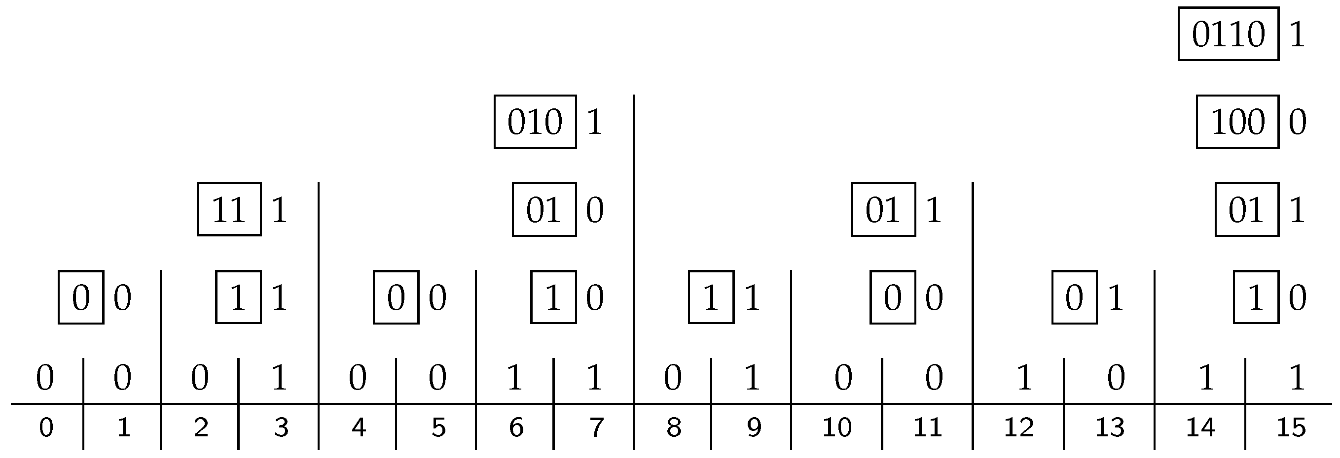
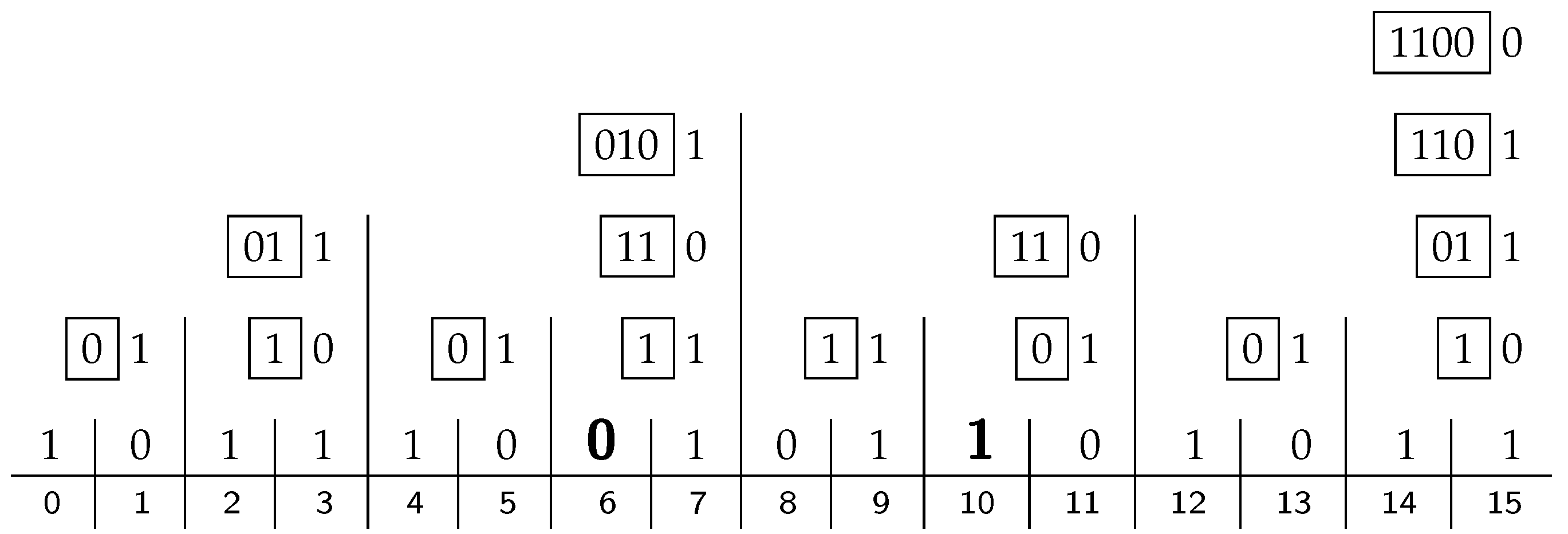
Continuing with the running example, Figure 3 shows the content of all the processors for the given input of size . We start with the bit-vector of Equation (1) in line 0, shown here immediately above the horizontal rule, including zeros at positions , which are substituting for the parity bits to be filled in. The indices of the bit positions are given below the rule. The ith line above line 0 shows the contents of the processors at level i, with the x bit right-justified, and the B-vector shown in a box to its left. The B vector in the top right corner contains the Hamming parity bits, which are 0110 in our case.
If these four parity bits are inserted in their proper places instead of the 0-stubs, as in Equation (2), we get the 15-bit Hamming code, encoding the eleven-bit data we started with. If this block is transmitted, it can be checked for errors by applying exactly the same apparatus again. The resulting code in the B vector on the top right will then be 0000, indicating that there is no error.
Suppose now that there is a single error in the block, namely at bit position 13. Applying once again the hierarchical structure of processors, the code in the top right B vector is 1101, which is the standard binary representation of the number 13—the index of the wrong bit. All that is left to do then is to flip the bit in the thirteenth bit position to restore the original input.
According to the parallel random-access-machine (PRAM) complexity model, the work of the hierarchical parallel Hamming code presented in Algorithm 1 for elements is , while the span is , using processors.
4. Full Exploitation of the Parallel Processing Power
If the size of the input block is doubled to , there is a tradeoff between the following options:
- adding only a single parity bit to the Hamming code, but still being able to correct only a single wrong bit among the bits that are given; or
- adding parity bits and immunizing each block of n input bits on its own against a single error.
While the above hierarchical scheme can be adapted to any size n of the input, this will obviously not be effective for very large n. Moreover, since only at the first step are all of the processors working (and only half of them at the next step, and then only a quarter, etc.), most of the processors are in fact idle most of the time. This can be rectified by using an interleaving schedule as suggested in [6].
Suppose a long sequence of data bits is given for which a Hamming code should be built. We shall process them in blocks of bits, for some . Each such block will be transformed into one of size n bits, including the parity bits and a bit in position 0. Denote the input blocks by , , and assume that the work of a single processor takes one unit of time.
In the description of the processing of a single block, the assumption was that processors are needed for the first step, and only a part of them for the other steps. We now assume that processors are available and show how—after time units—all of the processors can be kept busy all of the time. Refer to Figure 4 for a schematic picture of the assignments of processors to blocks as a function of the time units.
At time 1, processors are assigned to work on level 1 for the block . At time 2, processors will work on level 2 of , while other processors start working on level 1 for block . At time 3, the number of processors working will already be , etc. From time on, all the processors will be working in parallel. Block —which is emphasized in Figure 4—will be processed in the time interval from j to . Looking at the figure from another point of view, at time i, the processors work simultaneously on level 1 of , on level 2 of ,…, and on level of , as shown by the different shades of gray in Figure 4.
If the sequence of blocks is finite, the work on the last one starts at time N, and continues until time ; the processors will again be used only partially in these last time units, as shown at the right end of Figure 4. Note that might be negligible relative to N. For example, reasonable values could be to partition 1 GB of data into blocks of about 32,000 bits (i.e., ). This yields about blocks, and all the processors can be kept busy all of the time, except for the first and last 14 time units. The internal space needed for each processor would be 2 bytes, and according to the RAM model, the work performed by each processor takes time .
5. Double Error Detection
The Hamming error correcting scheme can be extended not only to correct single errors, but also to detect double errors at the price of a single additional parity bit. This can be implemented in the scheme described above almost for free.
The idea is to define—only for the highest level (indexed )—an additional bit y by
where and are the bits stored in the only processor of the top level; that is, are the parity bits as defined by Hamming, and is the parity of the entire set of data bits. For the example of Figure 3, and , so .
This additional bit y is then plugged into the extended bit-vector at position 0. Recall that this bit position was in fact empty, but has been added for ease of processing. Note that index 0 does not belong to any of the sets of indices forming the Hamming parity bits, so adding a bit in position 0 does not affect any of the boxed B vectors in the entire hierarchical procedure. Referring to Figure 3, replacing the 0-bit in position 0 by will flip all the x-bits on the leftmost branch of the binary tree (the path from the leaf in position 0 up to the root). In particular, the x-bit of the root will be 0.
This fact is not a coincidence, but will always hold if there is no error. To see why, assume that the n bits of the block are , denote the set of indices that are powers of two by , and denote by Q the set of complementing indices of the data bits, . Let X be the x-bit of the root. We then have
Using the definition of y in (3), we have that
which yields
If there is a single error, the X bit will be 1, as in the example of Figure 5, where we again flip all the x-bits on the leftmost branch. The index of the erroneous bit will be given in the B vector of the root. In this case, this B vector may consist only of zeros, indicating that the wrongly transmitted bit is y, in position 0. If , as in the given example, B is the index of the error and may thus be corrected.
If there is a double error, the X bit will again be 0, but the B vector cannot be zero. In fact, B will contain the XOR of the binary representations of the indices of the errors, and this XOR can only be 0 if the indices are equal. On the other hand, the B vector does not reveal enough information to know which bits are wrong, as there are several pairs of indices yielding the same XOR, so we have detection only, and not correction. The formal algorithm for the decoding is thus:
    if x = 0 then
      if B = 0 then   no error
      else            double error (no correction)
    else                single error at index represented by B
Figure 5 shows our running example with two errors in positions 6 and 10. Since
but
, we know that there are two errors, but are not able to correct them. The indices of the errors in binary are 0110 and 1010, and their XOR is 1100, which can be found in the B vector. However, a pair of errors at positions 9 and 5, or 13 and 1, would have given the same B vector, so all we can conclude is that there are (at least) two errors.
6. Conclusions
The Hamming code is a well-known error-correcting code in which data bits are secured by means of parity bits, allowing to recover from any single bit-flip error. Each of the parity bits is the result of the XORing of some subset of the data bits, and these subsets are chosen so as to let any bit position be defined by the intersection of some of the . A straightforward implementation of the Hamming code thus needs to handle the entire block of n data bits to extract the parity bits; that is, all the data and parity bits have to reside in memory simultaneously, and this is also true for the decoding phase: data and parity bits are processed together to check if some single error has occurred.
The contribution of this paper is the observation that this process may be parallelized in the sense of the hierarchy of processors defined in our model of Section 2.2. Actually, the entire process is summarized in Figure 2, depicting the basic building block of our suggested algorithm, which simply replicates the block in layers, times in the ith layer. The utterly simple work performed by such a block—the last two lines of Algorithm 1—is assigned to one of the processors and is the same for all the processors and all the layers, just with varying parameters. There is no need for any shared memory for the processors, nor is there any necessary inter-processor communication among the processors within the same layer. Processors of adjacent layers are connected by the hierarchy pattern described in Figure 1, where the outputs of a pair of neighboring processors of level i serve as input to a single processor of level , .
Author Contributions
There was equal contribution of both authors.
Conflicts of Interest
The authors declare no conflict of interest.
References
- Hamming, R.W. Error Detecting and Error Correcting Codes. Bell Syst. Tech. J. 1950, 29, 147–160. [Google Scholar] [CrossRef]
- Hirsch, M.; Klein, S.T.; Toaff, Y. Improving deduplication techniques by accelerating remainder calculations. Discret. Appl. Math. 2014, 163, 307–315. [Google Scholar] [CrossRef]
- Mitarai, H.; McCluskey, E.J. Design of a Parallel Encoder/Decoder for the Hamming Code, Using ROM; Technical Report CSL–TR–72–36; Stanford University: Stanford, CA, USA, 1972. [Google Scholar]
- Divsalar, D.; Dolinar, S. Concatenation of Hamming Codes and Accumulator Codes with High-Order Modulations for High-Speed Decoding; Jet Propulsion Laboratory (JPL): Pasadena, CA, USA, 2004; pp. 42–156. [Google Scholar]
- Islam, M.S.; Kim, C.H.; Kim, J. Computationally efficient implementation of a Hamming code decoder using Graphics Processing Unit. J. Commun. Netw. 2015, 17, 198–202. [Google Scholar] [CrossRef]
- Hirsch, M.; Klein, S.T.; Toaff, Y. Layouts for improved hierarchical parallel computations. J. Discret. Algorithms 2014, 28, 23–30. [Google Scholar] [CrossRef]
Figure 1.
Schematic representation of the hierarchical evaluation.
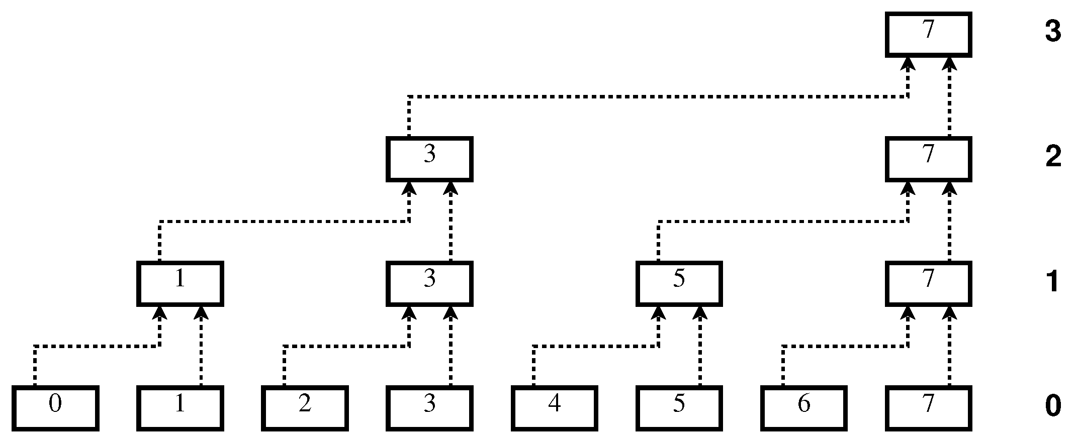
Figure 2.
Schematical view of the work of a single processor.
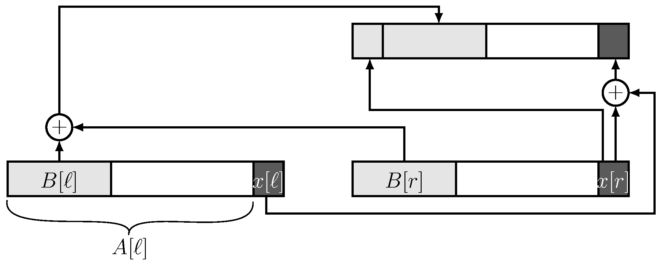
Figure 3.
Building the vector of parity bits.

Figure 4.
Assignments of processors and data blocks as a function of time.
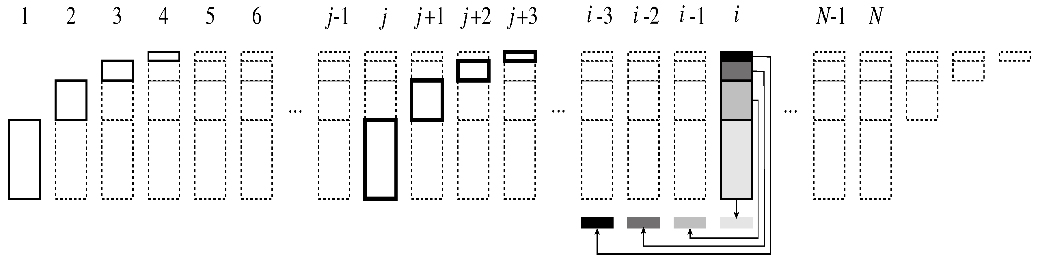
Figure 5.
Detecting a double error.
© 2017 by the authors. Licensee MDPI, Basel, Switzerland. This article is an open access article distributed under the terms and conditions of the Creative Commons Attribution (CC BY) license (http://creativecommons.org/licenses/by/4.0/).
Share and Cite
MDPI and ACS Style
Klein, S.T.; Shapira, D. Hierarchical Parallel Evaluation of a Hamming Code. Algorithms 2017, 10, 50. https://doi.org/10.3390/a10020050
AMA Style
Klein ST, Shapira D. Hierarchical Parallel Evaluation of a Hamming Code. Algorithms. 2017; 10(2):50. https://doi.org/10.3390/a10020050
Chicago/Turabian StyleKlein, Shmuel T., and Dana Shapira. 2017. "Hierarchical Parallel Evaluation of a Hamming Code" Algorithms 10, no. 2: 50. https://doi.org/10.3390/a10020050
Note that from the first issue of 2016, this journal uses article numbers instead of page numbers. See further details here.