
An Efficient Sixth-Order Newton-Type Method for Solving Nonlinear Systems


1
School of Mathematics and Physics, Bohai University, Jinzhou 121013, China
2
Department of Mathematics and Information Engineering, Puyang Vocational and Technical College, Puyang 457000, China
*
Author to whom correspondence should be addressed.
Algorithms 2017, 10(2), 45; https://doi.org/10.3390/a10020045
Submission received: 26 January 2017
/
Revised: 8 April 2017
/
Accepted: 20 April 2017
/
Published: 25 April 2017
(This article belongs to the Special Issue Numerical Algorithms for Solving Nonlinear Equations and Systems 2017)
Abstract
:In this paper, we present a new sixth-order iterative method for solving nonlinear systems and prove a local convergence result. The new method requires solving five linear systems per iteration. An important feature of the new method is that the LU (lower upper, also called LU factorization) decomposition of the Jacobian matrix is computed only once in each iteration. The computational efficiency index of the new method is compared to that of some known methods. Numerical results are given to show that the convergence behavior of the new method is similar to the existing methods. The new method can be applied to small- and medium-sized nonlinear systems.
1. Introduction
We consider the problem of finding a zero of a nonlinear function , that is, a solution of the nonlinear system with equations and unknowns. Newton’s method [1,2] is the well-known method for solving nonlinear systems, which can be written as:
where is the Jacobian matrix of the function evaluated in the iteration and is the inverse of . Newton’s method is denoted by NM. Newton’s method converges quadratically if is nonsingular and is Lipschitz continuous on . The method (1) can be written as:
which requires multiplications and divisions in the LU decomposition (lower upper, also called LU factorization) and multiplications and divisions for solving two triangular linear systems. So, the computational cost (multiplications and divisions) of the method (1) is
In order to accelerate the convergence or to reduce the computational cost and function evaluation in each step of the iterative process, many efficient methods have been proposed for solving nonlinear systems, see [3,4,5,6,7,8,9,10,11,12,13,14,15,16,17,18,19,20,21] and the references therein. Cordero et al. [3,4] developed some variants of Newton’s method. One of the methods is the following fourth-order method [3]:
where is the identity matrix. Method (3) is denoted by CM4 and requires LU decomposition of the Jacobian matrix only once per full iteration. Based on method (3), Cordero et al. [4] presented the following sixth-order method:
where is the identity matrix. Method (4) is denoted by CHM and requires two LU decompositions of the Jacobian matrix, one for and one for . Grau-Sánchez et al. [5] obtained the following sixth-order method:
where denotes the first-order divided difference of . Method (5) is denoted by SNAM and requires two LU decompositions for solving the linear systems involved.
It is well known that the computational cost of the iterative method greatly influences the efficiency of the iterative method. The number of LU decompositions that are used in the iterative method thus plays an important role when it comes to measuring the computational cost. So, we can reduce the computational cost of the iterative method by reducing the number of LU decompositions in each iteration.
The purpose of this paper is to construct a new sixth-order iterative method for solving small- and medium-sized systems. The theoretical advantages of the new method are based on the assumption that the Jacobian matrix is dense and that LU factorization is used to solve systems with the Jacobian. This assumption is not correct for sparse Jacobian matrices. An important feature of the new method is that the LU decomposition is computed only once per full iteration. This paper is organized as follows. In Section 2, based on the well-known fourth-order method (3), we present a sixth-order iterative method for solving nonlinear systems. The new method only increases one function evaluation, . For a system of equations, each iteration uses evaluations of scalar functions. The computational efficiency is compared to some well-known methods in Section 3. In Section 4, numerical examples are given to illustrate the convergence behavior of our method. Section 5 offers a short conclusion.
2. The New Method and Analysis of Convergence
Based on the method (3), we construct the following iterative scheme:
where is the identity matrix. We note that the first two steps of method (6) are the same as those of method (3), and the third step of method (6) increases one function evaluation . Method (6) will be denoted by M6. For method (6), we have the following convergence analysis.
Theorem 1.
Let be a solution of the system and be sufficiently differentiable in an open neighborhood of . Suppose that is nonsingular in Then, for an initial approximation sufficiently close to , the iterations converge with order 6.
Proof.
By using the notation introduced in [6], we have the following Taylor’s expansion of around :
where , , , and denotes . From (7) the derivatives of can be written as:
where . The inverse of (8) can be written as:
Solving system (11), we get:
then,
Let us denote From (6), (7) and (14), we arrive at:
By a similar argument to that of (7), we obtain:
From (14) and (17), we have:
Let us denote From (14), (15) and (18), we get:
Therefore, from (15) and (18)—(20), we obtain the error equation:
This implies that method (6) is of sixth-order convergence. This completes the proof.
In order to simplify the calculation, the new method (6) can be written as:
From (22), we can see that the LU decomposition of the Jacobian matrix would be computed only once per iteration.
3. Computational Efficiency
Here, we want to compare the computational efficiency index of our sixth-order method (M6, (6)) with Newton’s method (NM, (1)), Cordero’s fourth-order method (CM4, (3)), Grau-Sánchez’s sixth-order method (SNAM, (5)) and Cordero’s sixth-order methods (CHM, (4)) and (CTVM, (18)). The method CTVM [7] is as follows:
We define, respectively, the computational efficiency index () of the methods NM, CM4, SNAM, CHM, CTVM and M6 as:
where is the convergence order of the method and is the computational cost of method. The is given by [8]:
where represents the number of evaluations of the scalar functions used in the evaluations of , and . The represents the computational cost per iteration. is the ratio between multiplications (and divisions) and evaluations of functions that are required to express in terms of multiplications (and divisions). The divided difference is defined by [9]:
where and are computed separately. When we compute a divided difference, we need quotients and scalar function evaluations. We must add multiplications for the scalar product, multiplications for the matrix-vector multiplication and evaluations of scalar functions for any new derivative In order to factorize a matrix, we require multiplications and divisions in the LU decomposition. We require multiplications and divisions for solving two triangular linear systems.
Taking into account the previous considerations, we give the computational cost of each iterative method in Table 1.
From Table 1, we can see that these sixth-order iterative methods have the same number of function evaluations. Our method (M6) needs less LU decompositions than other methods with the same order. Therefore, the computational cost of our method is lower.
We use the following expressions [10] to compare the computational efficiency index of each iterative method:
For the iterative method is more efficient than We have the following theorem:
Theorem 2.
For all we have:
- 1.
- for all
- 2.
- for all
- 3.
- for all
Proof.
We note that the methods SNAM, CHM, CTVM and method M6 have the same order and the same number of function evaluations
- Based on the expression (26), the relation between SNAM and M6 can be given by:Subtracting the denominator from the numerator of (27), we have:Equation (28) is positive for Thus, we get for all and
- The relation between CHM and M6 is given by:Subtracting the denominator from the numerator of (29), we have:Equation (30) is positive for Thus, we get for all and
- The relation between CHM and M6 can be given by:Subtracting the denominator from the numerator of (31), we have:Equation (32) is positive for Thus, we obtain for all and . This completes the proof.
Theorem 3.
For all we have:
- 1.
- for all
- 2.
- for all
Proof.
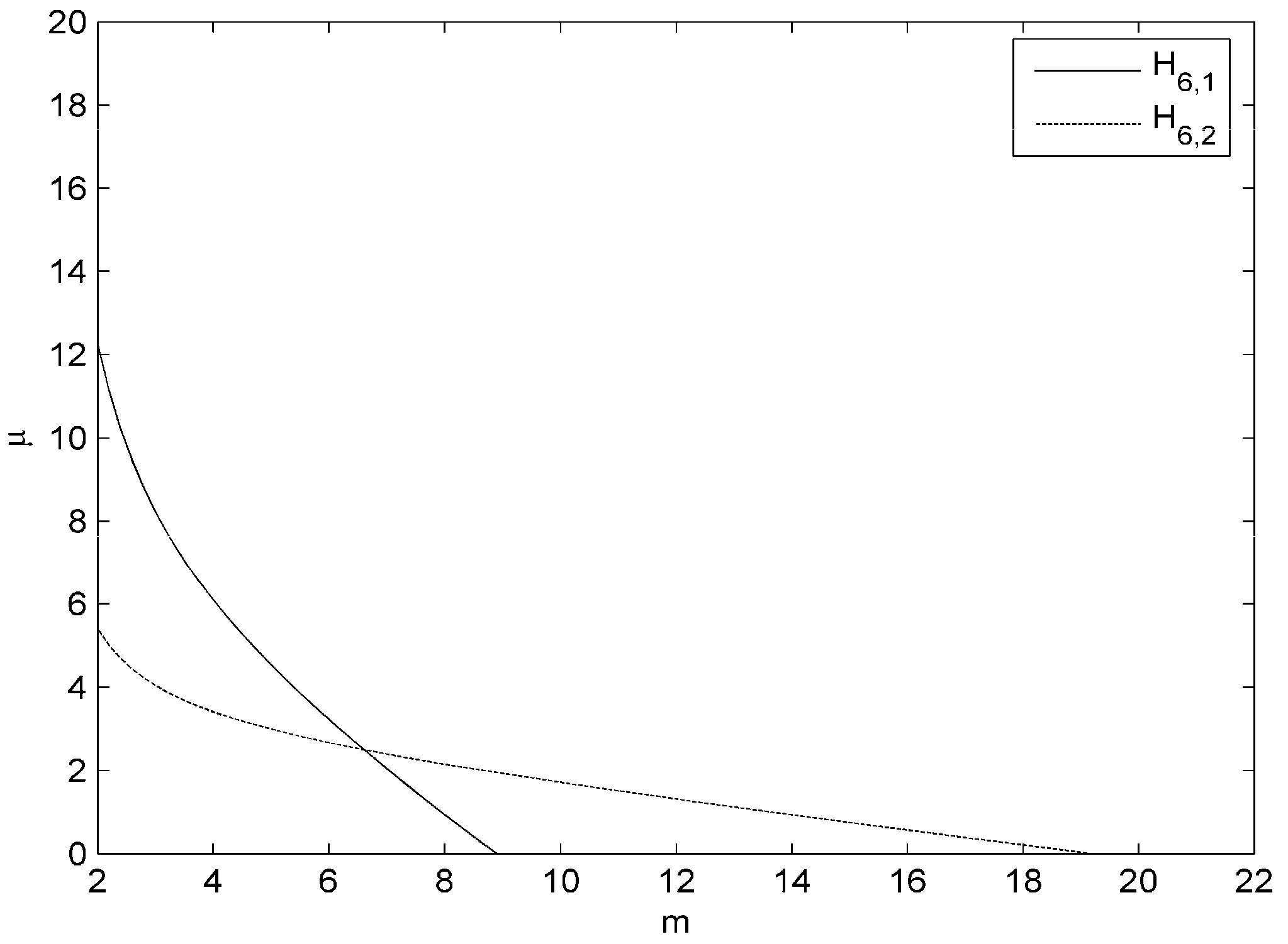
- From expression (26) and Table 1, we get the following relation between NM and M6:We consider the boundary . The boundary can be given by the following equation:where over it (see Figure 1). Boundary (34) cuts axes at points and . Thus, we get since for all and
- The relation between CM4 and M6 is given by:We consider the boundary . The boundary can be given by the following equation:where over it (see Figure 1). Boundary (36) cuts axes at points and . Thus, we get since for all and
This completes the proof.
4. Numerical Examples
In this section, we compare the related methods by numerical experiments. The numerical experiments are performed using the MAPLE computer algebra system with 2048 digits. The method M6 is compared with NM, CM4, SNAM, CHM, CTVM by solving some nonlinear systems. The stopping criterion used is or .
Following nonlinear systems are used:
and the initial value is The solution is .
and the initial value is The solution is
where and such that
When is odd, the exact zeros of are and The initial value is
Table 4 presents the results showing the following information: the number of iterations needed to converge to the solution, the value of the stopping factors at the last step and the computational order of convergence . The computational order of convergence is defined by [18]:
The numerical results shown in Table 4 are in concordance with the theory developed in this paper. The order of convergence of our method (M6) is 6, which is higher than the methods NM and CM4. The iterative method SNAM is not convergent (nc) for with the corresponding initial value. The convergence behavior of our method is similar to the existing methods in this paper.
5. Conclusions
In this paper, we have proposed a new iterative method of order six for solving nonlinear systems. Although five linear systems are required to be solved in each iteration, the LU decomposition of the linear systems are computed only once per full iteration. Numerical results are given to show that our method has a similar convergence behavior as the existing methods in this paper. The new method is suitable for solving small- and medium-sized systems. In order to obtain an efficient iterative method for solving nonlinear systems, we should make the iterative method achieve an as high as possible convergence order consuming an as small as possible computational cost. In addition, the theoretical advantages of the new method are based on the assumption that the Jacobian matrix is dense and that LU factorization is used to solve the systems with the Jacobian. This assumption is not correct for sparse Jacobian matrices.
Acknowledgments
This project is supported by the National Natural Science Foundation of China (Nos. 11547005 and 61572082), the PhD Start-up Fund of Liaoning Province of China (No. 201501196) and the Educational Commission Foundation of Liaoning Province of China (No. L2015012).
Author Contributions
Xiaofeng Wang conceived and designed the experiments; Yang Li performed the experiments; Xiaofeng Wang wrote the paper.
Conflicts of Interest
The authors declare no conflict of interest.
References
- Kelley, C.T. Solving Nonlinear Equations with Newton’s Method; SIAM: Philadelphia, PA, USA, 2003. [Google Scholar]
- Ortega, J.M.; Rheinbolt, W.C. Iterative Solution of Nonlinear Equations in Several Variables; Academic Press: New York, NY, USA, 1970. [Google Scholar]
- Cordero, A.; Martínez, E.; Torregrosa, J.R. Iterative methods of order four and five for systems of nonlinear equations. J. Comput. Appl. Math. 2009, 231, 541–551. [Google Scholar] [CrossRef]
- Cordero, A.; Hueso, J.L.; Matínez, E.; Torregrosa, J.R. Increasing the convergence order of an iterative method for nonlinear systems. Appl. Math. Lett. 2012, 25, 2369–2374. [Google Scholar] [CrossRef]
- Sánchez, M.G.; Noguera, M.; Amat, S. On the approximation of derivatives using divided difference operators preserving the local convergence order of iterative methods. J. Comput. Appl. Math. 2013, 237, 263–272. [Google Scholar]
- Cordero, A.; Hueso, J.L.; Matínez, E.; Torregrosa, J.R. Efficient high-order methods based on golden ratio for nonlinear systems. Appl. Math. Comput. 2011, 217, 4548–4556. [Google Scholar] [CrossRef]
- Cordero, A.; Torregrosa, J.R.; Vassileva, M.P. Pseudocomposition: A technique to design predictor-corrector methods for systems of nonlinear equations. Appl. Math. Comput. 2012, 218, 11496–11504. [Google Scholar] [CrossRef]
- Ezquerro, J.A.; Grau, À.; Sánchez, M.G.; Hernández, M.A. On the efficiency of two variants of Kurchatov’s method for solving nonlinear systems. Numer. Algorithms 2013, 64, 685–698. [Google Scholar] [CrossRef]
- Potra, F.A.; Pták, V. Nondiscrete Induction and Iterative Processes; Pitman Publishing: Boston, MA, USA, 1984. [Google Scholar]
- Ezquerro, J.A.; Grau, À.; Sánchez, M.G.; Hernández, M.A.; Noguera, M. Analysing the efficiency of some modifications of the secant method. Comput. Math. Appl. 2012, 64, 2066–2073. [Google Scholar] [CrossRef]
- Sánchez, M.G.; Grau, À.; Noguera, M. On the computational efficiency index and some iterative methods for solving systems of nonlinear equations. J. Comput. Appl. Math. 2011, 236, 1259–1266. [Google Scholar] [CrossRef]
- Sánchez, M.G.; Grau, À.; Noguera, M. Frozen divided difference scheme for solving systems of nonlinear equations. J. Comput. Appl. Math. 2011, 235, 739–1743. [Google Scholar]
- Ezquerro, J.A.; Hernández, M.A.; Romero, N. Solving nonlinear integral equations of Fredholm type with high order iterative methods. J. Comput. Appl. Math. 2011, 236, 1449–1463. [Google Scholar] [CrossRef]
- Argyros, I.K.; Hilout, S. On the local convergence of fast two-step Newton-like methods for solving nonlinear equations. J. Comput. Appl. Math. 2013, 245, 1–9. [Google Scholar] [CrossRef]
- Amat, S.; Busquier, S.; Grau, À.; Sánchez, M.G. Maximum efficiency for a family of Newton-like methods with frozen derivatives and some applications. Appl. Math. Comput. 2013, 219, 7954–7963. [Google Scholar] [CrossRef]
- Wang, X.; Zhang, T. A family of Steffensen type methods with seventh-order convergence. Numer. Algorithms 2013, 62, 429–444. [Google Scholar] [CrossRef]
- Sharma, J.R.; Guha, R.K.; Sharma, R. An efficient fourth order weighted-Newton method for systems of nonlinear equations. Numer. Algorithms 2013, 62, 307–323. [Google Scholar] [CrossRef]
- Weerakoon, S.; Fernando, T.G.I. A variant of Newton’s method with accelerated third-order convergence. Appl. Math. Lett. 2000, 13, 87–93. [Google Scholar] [CrossRef]
- Wang, X.; Zhang, T.; Qian, W.; Teng, M. Seventh-order derivative-free iterative method for solving nonlinear systems. Numer. Algorithms 2015, 70, 545–558. [Google Scholar] [CrossRef]
- Păvăloiu, I. On approximating the inverse of a matrix. Creative Math. 2003, 12, 15–20. [Google Scholar]
- Diaconu, A.; Păvăloiu, I. Asupra unor metode iterative pentru rezolvarea ecuaţiilor operaţionale neliniare. Rev. Anal. Numer. Teor. Aproximaţiei 1973, 2, 61–69. [Google Scholar]
Figure 1.
The boundary functions and in —plain.


Table 1.
Computational cost of the iterative methods.
| Methods | ||||
|---|---|---|---|---|
| NM | 2 | |||
| CM4 | 4 | |||
| SNAM | 6 | |||
| CHM | 6 | |||
| CTVM | 6 | |||
| M6 | 6 |
Table 2.
Computational efficiency indices of the methods .
| 5 | 1.0055606 | 1.0052450 | 1.0049895 | 1.0052838 | 1.0055283 | 1.0050600 |
| 7 | 1.0025422 | 1.0025753 | 1.0023729 | 1.0025126 | 1.0026423 | 1.0025375 |
| 9 | 1.0013845 | 1.0014870 | 1.0013340 | 1.0014096 | 1.0014831 | 1.0014905 |
| 11 | 1.0008405 | 1.0009480 | 1.0008314 | 1.0008761 | 1.0009207 | 1.0009643 |
| 20 | 1.0001777 | 1.0002326 | 1.0001898 | 1.0001978 | 1.0002060 | 1.0002482 |
| 50 | 1.0000141 | 1.0000224 | 1.0000165 | 1.0000169 | 1.0000173 | 1.0000258 |
| 100 | 1.0000019 | 1.0000034 | 1.0000023 | 1.0000024 | 1.0000024 | 1.0000040 |
| 200 | 1.0000002 | 1.0000005 | 1.0000003 | 1.0000003 | 1.0000003 | 1.0000006 |
Table 3.
Computational efficiency indices of the methods ().
| 5 | 1.0028332 | 1.0027489 | 1.0028941 | 1.0029907 | 1.0030675 | 1.0029177 |
| 7 | 1.0013956 | 1.0014055 | 1.0014554 | 1.0015068 | 1.0015525 | 1.0015157 |
| 9 | 1.0008054 | 1.0008390 | 1.0008536 | 1.0008839 | 1.0009123 | 1.0009150 |
| 11 | 1.0005124 | 1.0005505 | 1.0005504 | 1.0005697 | 1.0005882 | 1.0006057 |
| 20 | 1.0001242 | 1.0001488 | 1.0001391 | 1.0001434 | 1.0001476 | 1.0001681 |
| 50 | 1.0000117 | 1.0000168 | 1.0000139 | 1.0000141 | 1.0000144 | 1.0000199 |
| 100 | 1.0000017 | 1.0000028 | 1.0000021 | 1.0000021 | 1.0000022 | 1.0000034 |
| 200 | 1.0000002 | 1.0000004 | 1.0000003 | 1.0000003 | 1.0000003 | 1.0000005 |
Table 4.
Numerical results for by the methods.
| Function | Method | ||||
|---|---|---|---|---|---|
| NM | 8 | 2.42128 × 10−192 | 1.06480 × 10−383 | 1.99667 | |
| CM4 | 5 | 5.59843 × 10−147 | 2.69120 × 10−586 | 4.00129 | |
| SNAM | 4 | 3.76810 × 10−39 | 3.25655 × 10−227 | 6.09363 | |
| CHM | 4 | 4.18959 × 10−123 | 4.03125 × 10−736 | 5.99962 | |
| CTVM | 4 | 2.07203 × 10−100 | 2.63883 × 10−597 | 6.00033 | |
| M6 | 4 | 7.65662 × 10−119 | 1.55028 × 10−710 | 6.00589 | |
| NM | 9 | 3.41596 × 10−116 | 2.48971 × 10−232 | 1.97549 | |
| CM4 | 5 | 3.73825 × 10−90 | 1.20501 × 10−359 | 4.02761 | |
| SNAM | 4 | 9.18821 × 10⁻³⁵ | 6.76819 × 10−207 | 5.98999 | |
| CHM | 4 | 8.31995 × 10−52 | 8.11818 × 10−310 | 5.72008 | |
| CTVM | 4 | 3.82928 × 10−42 | 4.59455 × 10−251 | 5.85429 | |
| M6 | 4 | 8.13364 × 10−65 | 6.14607 × 10−387 | 5.99644 | |
| NM | 22 | 2.71070 × 10−196 | 2.20459 × 10−392 | 1.99900 | |
| CM4 | 6 | 2.26562 × 10−115 | 1.03777 × 10−460 | 4.00061 | |
| SNAM | nc | ||||
| CHM | 5 | 2.79450 × 10−99 | 4.68047 × 10−594 | 5.92903 | |
| CTVM | 5 | 5.12075 × 10−193 | 1.30600 × 10−1157 | 5.97091 | |
| M6 | 5 | 1.99499 × 10−161 | 3.41913 × 10−967 | 6.08153 |
© 2017 by the authors. Licensee MDPI, Basel, Switzerland. This article is an open access article distributed under the terms and conditions of the Creative Commons Attribution (CC BY) license (http://creativecommons.org/licenses/by/4.0/).
Share and Cite
MDPI and ACS Style
Wang, X.; Li, Y. An Efficient Sixth-Order Newton-Type Method for Solving Nonlinear Systems. Algorithms 2017, 10, 45. https://doi.org/10.3390/a10020045
AMA Style
Wang X, Li Y. An Efficient Sixth-Order Newton-Type Method for Solving Nonlinear Systems. Algorithms. 2017; 10(2):45. https://doi.org/10.3390/a10020045
Chicago/Turabian StyleWang, Xiaofeng, and Yang Li. 2017. "An Efficient Sixth-Order Newton-Type Method for Solving Nonlinear Systems" Algorithms 10, no. 2: 45. https://doi.org/10.3390/a10020045
Note that from the first issue of 2016, this journal uses article numbers instead of page numbers. See further details here.