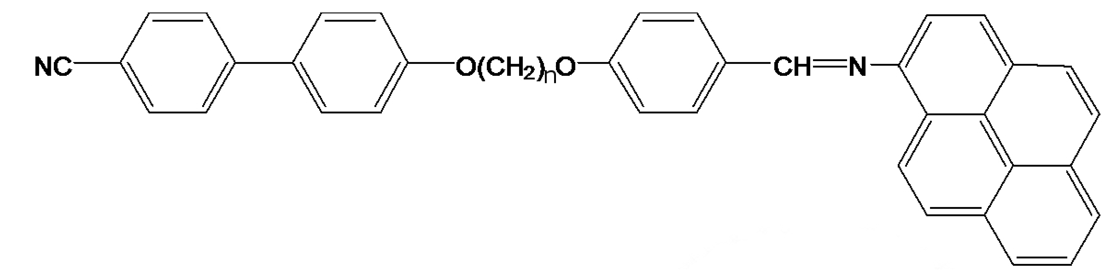
The liquid crystal dimer, CBO11O.Py, consists of a cyanobiphenyl group attached to a pyreniminebenzylidene group via a flexible spacer of 11 methylene units, as shown in
Figure 1. The interest to study the CBOnO.Py series of dimers (n accounts for the number of methylene groups), first prepared by Attard
et al. [
24], came from the combination of the mesogenic and electrooptic properties of the cyanobiphenyls and the glassy behavior of the pyrene, localized in the imine-based core. In fact, although these dimers do present such properties, for the case of our particular compound, CBO11O.Py, the nematic glassy state is only accessible under high cooling rates (15 K·min
−1 or higher) [
22]. In order to overcome this inconvenience, we introduce a quenched random disorder in the material by the dispersion of γ-alumina nanoparticles, which partially suppress the undesired crystallization of the liquid crystal dimer.
Figure 1.
CBOnO.Py molecule.
2.1. Thermal Behavior
The N phase of CBO11O.Py can be supercooled and, eventually, frozen to the corresponding nematic glassy state [
22,
23]. With the sample in the nematic glassy state, heating up allows us to observe the glass transition and, at about 15 K above
Tg, the supercooled N phase crystallizes irreversibly. Afterwards, the transitions from crystal to nematic (Cr-N) and from nematic to isotropic (N-I) take place at the corresponding transition temperatures (
TCrN,
TNI). These temperatures, together with
Tg, taken from [
22,
23], are listed in
Table 1.
Table 1.
Phase transition temperatures, Tg, TCrN, TCrI and TNI for the bulk and confined system CBO11O.Py + γ-alumina. All temperatures have been recorded on heating.
Table 1.
Phase transition temperatures, Tg, TCrN, TCrI and TNI for the bulk and confined system CBO11O.Py + γ-alumina. All temperatures have been recorded on heating.
| ρs (g·cm−3) | TNI (K) | TCrN (K) | TCrI (K) | Tg (K) |
|---|
| 0 | 426.9 | 421.3 | – | 305.0 |
| 0.05 | 425.5 | 421.1 | – | 303.6 |
| 0.16 | 421.2 | – | 419.7 | 302.3 |
| 0.23 | 418.9 | – | 419.2 | 301.3 |
| 0.31 | 416.9 | – | 418.3 | 300.7 |
| 0.39 | 413.8 | – | 417.3 | 298.8 |
Some interesting effects arise when introducing γ-alumina nanoparticles in the host dimer.
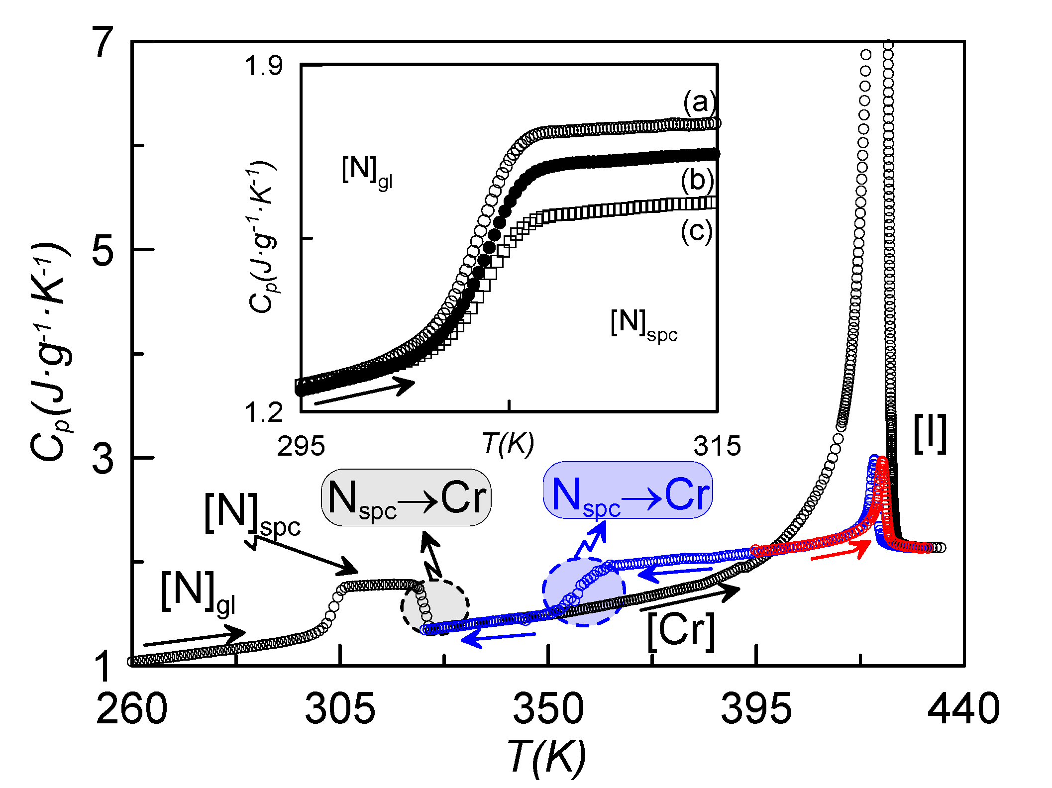
Figure 2 shows, as an example, the temperature dependence of the specific heat for the sample with ρ
s = 0.16 g·cm
−3, recorded at a rate of 1 K·min
−1, coming from different initial states. When cooling down at slow rates (1 K·min
−1) from the isotropic phase, the I-N-Cr phase sequence is obtained (blue curve, N
spc-Cr), with the nematic range being about 20 K larger than in the bulk sample under the same conditions of measurement. If we stop cooling at a temperature before crystallization takes place and heat the sample up from the N mesophase, the N-I phase transition takes place (red curve). If we cool the sample down from the isotropic phase at high enough rates, crystallization is avoided (or partially avoided) and we obtain the N glassy state. The black curve in
Figure 2 represents the heating run from the N glassy state up to the isotropic phase. The glass transition, crystallization and melting from the crystalline state directly to the isotropic phase are clearly observed. This indicates that the N phase becomes monotropic under the influence of the γ-alumina nanoparticles. This phenomenon is observed for concentrations above 0.1 g·cm
−3. Thus, the nematic phase is only present when cooling from the isotropic phase, and cannot be reached when heating from the crystalline state.
Figure 2.
Specific heat vs. temperature for the ρs = 0.16 g·cm−3; cooling down from the isotropic phase (blue curve), heating up from the nematic phase (red curve); heating up from the N glassy state after coming from the isotropic phase at high cooling rates (black curve). The inset shows the specific heat jump at the glass transition for the sample ρs = 0.16 g·cm−3, after having cooled the sample down at different rates: (a) 20 K·min−1, (b) 15 K·min−1, (c) 10 K·min−1. All measurements were recorded at a rate of 1 K·min−1.
The inset of
Figure 2 shows the characteristic specific heat jump, on heating at a rate of 1 K·min
−1, assigned to the glass transition obtained for the sample ρ
s = 0.16 g·cm
−3, previously cooled at different rates. The case denoted by (c) corresponds to the lower cooling rate (10 K·min
−1) with a smaller specific heat jump, which gets larger as the cooling rate increases. This is understandable by the fact that, if the cooling rate is not high enough, the sample tends to crystallize partially. This behavior was already observed for other LC dimers [
14]. The part remaining in the N phase ultimately becomes glassy at
Tg. All the more, as the concentration of nanoparticles is increased, the minimum cooling rate required to get the sample partially in the N glassy state decreases, from ~15 K·min
−1 for bulk CBO11O.Py down to 5 K·min
−1 for concentrations up to 0.23 g·cm
−3 and higher (for ρ
s = 0.16 g·cm
−3, this minimum cooling rate is about 10 K·min
−1).
Figure 2 shows the specific heat
vs. temperature around the N-I phase transition for bulk CBO11O.Py and some of the confined samples. As expected, the dispersion of nanoparticles induces a downward shift in the N-I phase transition temperature together with a suppressed and rounded specific heat peak similar to what is found for other liquid crystals under confinement [
26,
28,
29,
30,
31]. This effect can be translated to the other phase transitions (N
g-N
spc, Cr-N and Cr-I), but the depression in temperature is lesser. The transition temperatures,
Tg,
TCrN,
TCrI and
TNI, are listed in
Table 1 for the different samples. The dependence with concentration of the absolute value of the depression of the phase transition temperatures divided by the bulk transition temperature (from now on, normalized change of the phase transition temperature) is represented in the inset of
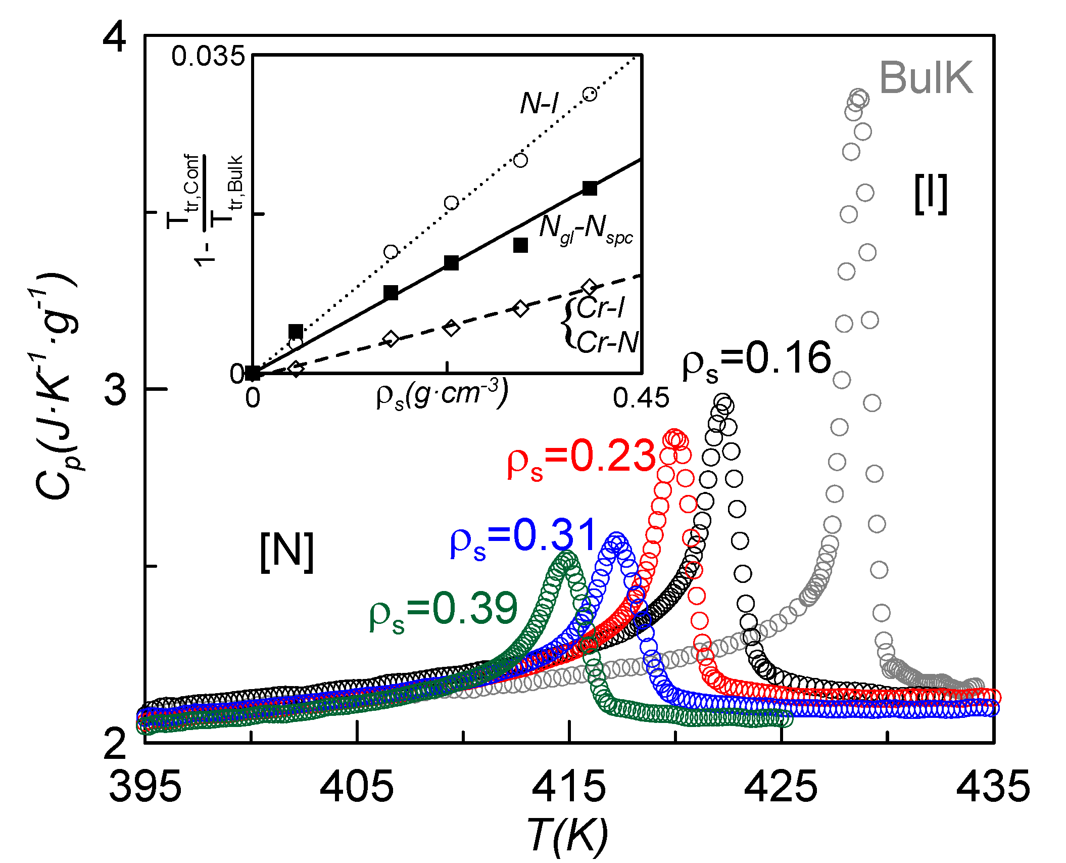
Figure 3. These values show a linear dependence with the nanoparticles concentration of the normalized change of the N-I phase transition temperature. Such a linear dependence is fitted to the relationship
where
A = 0.078 cm
3·g
−1. This behavior differs substantially from that of the 4O.8 monomer confined via the dispersion of the same γ-alumina nanoparticles [
26], in which the dependence was not linear. Such a difference could be explained by arguing that, since the CBO11O.Py molecule is larger and more flexible than the 4O.8 one, more dispersive material is needed to induce similar changes in the transition temperatures in the former with respect to the latter. Taking into account concentrations of γ-alumina below 0.1 g·cm
−3 in 4O.8, the normalized change of temperature with concentration is well fitted by a linear law [Equation (1)], with a value of
A equal to 0.28 cm
3·g
−1, about 3.6 times higher than the one corresponding to CBO11O.Py. This confirms the exposed argument. When the concentration of γ-alumina in 4O.8 goes over 0.1 g·cm
−3, the influence of the marginal nanoparticle is less every time and a kind of saturation takes place, giving rise to a non-linear relationship [
26]. In the case of CBO11O.Py, the used concentrations of γ-alumina are not enough to saturate.
Figure 3.
Specific heat vs. temperature for the six samples around the N-I phase transition. The inset shows the dependence of the absolute value of the depression of the normalized change of the phase transition temperatures (Tg, TCrN, TCrI and TNI) with concentration.
Figure 3.
Specific heat vs. temperature for the six samples around the N-I phase transition. The inset shows the dependence of the absolute value of the depression of the normalized change of the phase transition temperatures (Tg, TCrN, TCrI and TNI) with concentration.
The inset of
Figure 3 also shows the normalized change for the melting and glass transition temperatures
vs. nanoparticle concentration, which can also be fitted by a linear relationship as Equation (1). The values of the fitting constants
A are 0.023 cm
3·g
−1 for the melting temperature and 0.051 cm
3·g
−1 for the glass transition temperature. These values are about 1/3 and 2/3, respectively, of the corresponding value for the N-I phase transition. The isotropic and nematic phases are much more fluid than the N glassy state. These differences in viscosity make the N-I phase transition more sensitive to the influence of the presence of γ-alumina than the glass transition. The crystal to fluid-like phase transition seems to be affected by confinement in a lesser extent than the N
gl-N
spc phase transition. In our opinion, the order of the phase plays an important role.
2.2. Dielectric Measurements
The dielectric behavior of bulk CBO11O.Py far from the glass transition has already been published [
22,
23]. The crystallization of the sample 75 K above
Tg prevents a dielectric study close to the glass transition. The partial suppression of crystallization by the dispersion of γ-alumina nanoparticles in the host LC allows us to study the LC dimer dielectrically, reducing the forbidden temperature gap. Nevertheless, confinement could alter the molecular dynamics of the bulk liquid crystal and, therefore, a comparison is carried out below. Among the prepared confined samples, the one with ρ
s = 0.23 g·cm
−3 is chosen for our dielectric study, because higher concentrations have a similar impact in the suppression of crystallization.
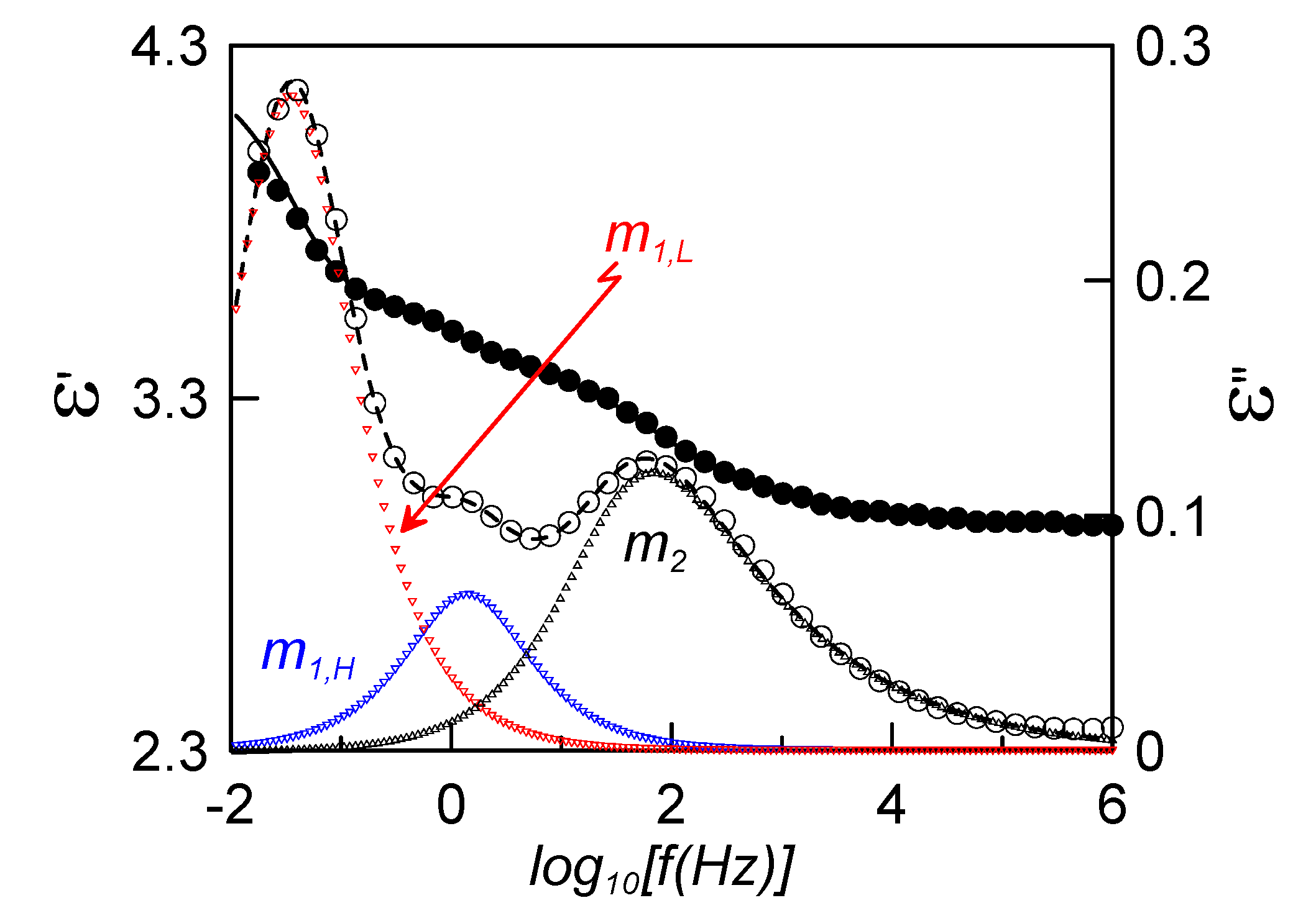
Figure 4 shows the real (full circles) and imaginary (empty circles) parts of the complex dielectric permittivity in the nematic phase at 313 K, for the confined sample with a DC bias of 20 V. It must be said that if no bias is applied, the sample adopts a mixed alignment, whereas the application of the DC bias increases the molecular alignment parallel to the probing electric field (homeotropic-like alignment).
Figure 4.
Frequency dependence of the complex dielectric permittivity for the sample ρs = 0.23 g·cm−3 at 313 K (N mesophase) under a DC bias of 20 V. Full circles account for the experimental real part, empty circles for the experimental imaginary part; fittings to Equation (2) are shown by the continuous (real part) and dashed (imaginary part) lines. Triangles represent the deconvoluted relaxation modes from the fitting.
Solid lines in
Figure 4 correspond to the fittings of experimental data to the empirical function:
where
k accounts for the relaxation modes present in the phase and each one is fitted according to the Havriliak-Negami function; Δε
k and τ
k are the dielectric strength and the relaxation time related to the frequency of maximum dielectric loss, respectively; α
k and β
k are parameters that describe the shape (width and symmetry) of the relaxation spectra;
is the dielectric permittivity at high frequencies (but lower than those corresponding to atomic and electronic resonance phenomena); and σ
DC is the electric conductivity. With respect to the α
k and β
k parameters, both are equal to 1 in the simplest (Debye) model. If the relaxation is more complex, the shape of the peaks may get broader (α
k < 1) and/or asymmetric (β
k ≠ 1). The system in the homeotropic-like alignment presents three relaxation modes in the N phase, just as the bulk material [
22]. Thus, the explanation of these modes will be in the same way, according to Sttochero’s theoretical model for the dielectric behavior of non-symmetric LC dimers [
20]. According to this model, the lowest frequency mode, m
1L, is identified due to the flip-flop motion of the pyrene group, which immediately forces the cyanobiphenyl unit to reorient and, therefore, it can be detected dielectrically. The intermediate frequency mode, m
1H, is related to the flip-flop reorientation of the cyanobiphenyl unit. The highest frequency mode, m
2, is due to precessions of the cyanobiphenyl group around the nematic director. Far from the glass transition, the two modes with lower frequencies, m
1L and m
1H, are Debye-like. The high frequency mode, m
2, is Cole-Cole (α
2 < 1 and β
2 = 1), with the parameter α
2 ranging from ~0.8 to ~0.5 as the compound is cooled down from the isotropic phase.
The shape of the relaxation modes changes deeply when approaching the glass transition. The molecular reorientations experiment huge steric couplings and become more cooperative. Both
α1L and
α1H decrease to 0.9, while the change is more obvious in the high frequency mode, where there is not just a modification in width but also in symmetry (α
2 ~ 0.8 and β
2 ~ 0.5). This phenomenon is typical for glass-forming materials when approaching the glass transition [
4,
8].
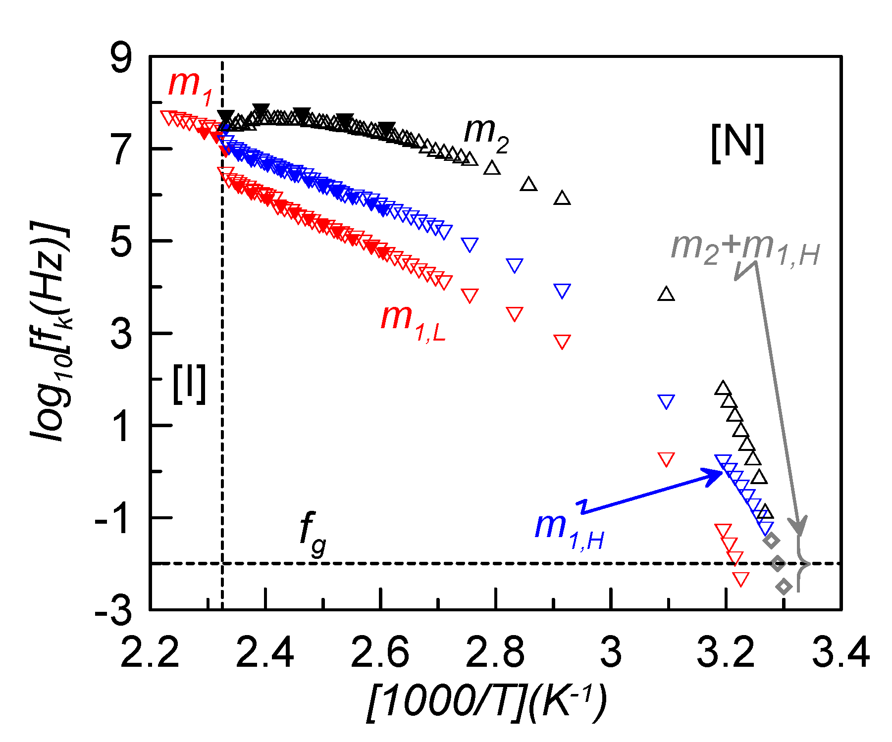
In the present study, the main interest consists in evaluating how the relaxation frequency of the maximum dielectric loss changes with temperature. This is presented in the Arrhenius plot of
Figure 5, where some values for bulk CBO11O.Py (full symbols) are also shown for comparison [
22]. First of all, it can be seen how the frequencies of bulk and confined samples do not differ significantly, so the dispersion of γ-alumina nanoparticles does not seem to noticeably affect the relaxation frequency of the modes.
Figure 5.
Arrhenius plot of the relaxation frequencies of the different elementary contributions for the sample ρ
s = 0.23 g·cm
−3 (empty symbols). For comparison purposes, results for bulk CBO11O.Py from reference [
22] are also shown (full symbols).
Figure 5.
Arrhenius plot of the relaxation frequencies of the different elementary contributions for the sample ρ
s = 0.23 g·cm
−3 (empty symbols). For comparison purposes, results for bulk CBO11O.Py from reference [
22] are also shown (full symbols).
For dielectric relaxations, a glass transition (denoted as dynamic glass transition) is obtained when the characteristic relaxation time,
τk, reaches about 100 s, or the corresponding frequency is approximately 10 mHz. As is clearly observed in
Figure 5, m
2 and m
1H relaxation modes tend to overlap in frequency when approaching the glass transition. At a low enough temperature, both modes are indistinguishable and the observed dielectric peak is attributed to a superposition of both. The fitting of this complex mode (grey symbols in
Figure 5) leads to a very asymmetric Cole-Davidson relaxation (α = 1, β = 0.3). This behavior is comparable to that found for the symmetric LC dimer, CB7CB, in which the twist-bend nematic (N
TB) mesophase is frozen and, at the glass transition, the two observed relaxation modes overlap [
11]. However, in the present case, the low frequency mode, m
1L, is observed separated from the other two and gets frozen at a temperature about 7 K higher. This would mean that, from a dielectric point of view, two glass transition temperatures involving different molecular motions seem to be present. As the lower in temperature glass transition is due to the dynamic disorder of the cyanobiphenyl group and the higher one is due to the pyrene reorientations, we denote both glass transition temperatures as
TgCB ~ 304 K and
TgPy ~ 311 K. The nematic environment at these low temperatures makes the steric interactions of each group much stronger in the case of the pyrene reorientations, which become more hindered and need more thermal energy to be activated and, accordingly,
TgPy >
TgCB.
The question that now arises is if it is possible to certify the existence of this double glass transition by other experimental techniques.
2.3. Thermal Stimulated Depolarization Currents (TSDC)
The unexpected dielectric results near the glass transition leads us to make a complementary analysis by means of Thermal Stimulated Depolarization Currents (TSDC). This technique is particularly well-suited for this analysis because it is equivalent to a very low frequency dielectric measurement [
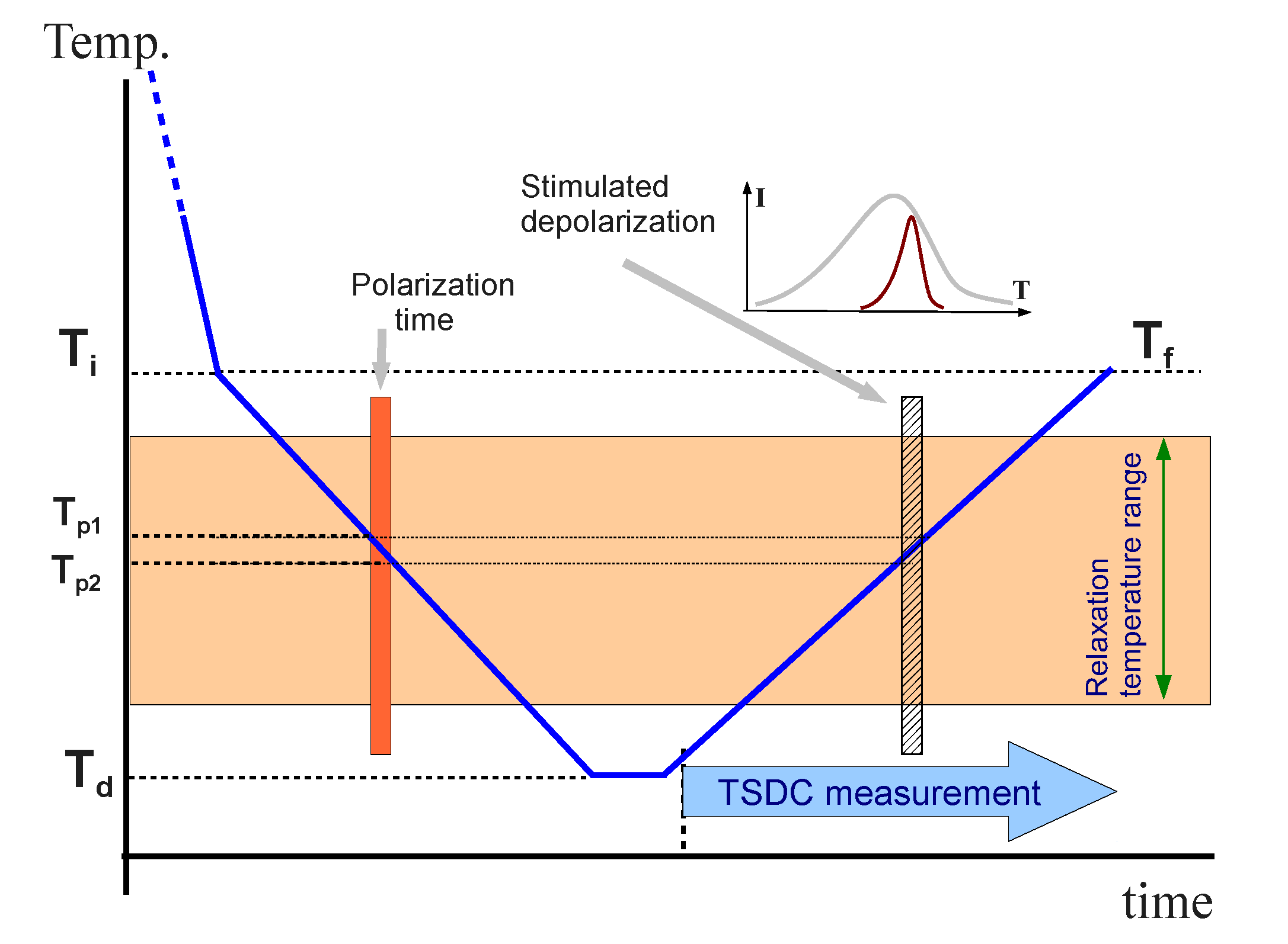
32]. TSDC measurements were performed by means of the so-called non-isothermal windowing (NIW) polarization method, in which the poling field is applied during a cooling ramp [
33,
34]. In our measurements the samples were cooled from the isotropic phase down to 325 K (
Ti) at a fast cooling rate (30 K·min
−1). They were held at this temperature for one minute and then cooled down to the deposit temperature (
Td = 275 K) at 2.5 K·min
−1. Within this second ramp, a static poling field was applied to polarize the material, from an initial temperature T
p1 to a final temperature
Tp2 <
Tp1. The sample was held at the deposit temperature for 15 minutes and, afterwards, it was heated again up to 325 K (
Tf) at 2.5 K·min
−1. During the heating ramp, the depolarization current was registered.
This experimental technique allows the deconvolution of a complex relaxation spectrum into its elementary components, using a methodology known as the Relaxation Map Analysis (RMA) [
33,
34]. In a RMA, elementary spectra can be obtained if the electric field is applied only in a very small temperature range during the cooling ramp. By this way only those motions (modes) that are activated at the poling temperature can lead to some polarization at the end of the cooling ramp. So, the obtained depolarization current obtained may be associated with the elementary mode activated at the poling temperature. The entire relaxation spectrum results from the superposition of the elementary modes obtained at different polarization temperatures. In a polymer, for example, it is possible to analyze the dominant structural relaxation, the α relaxation, which accounts for the global molecular reorientations, and resolve it into its simpler components [
33,
34].
Figure 6 shows the thermal diagram of a TSDC measurement.
Figure 6.
Diagram of a TSDC measurement.
Figure 6.
Diagram of a TSDC measurement.
In this work, we apply the TSDC technique to our confined LC dimer, in order to confirm the dielectric results. In the RMA analysis, we perform different NIW measurements, changing
Tp1 and
Tp2 in each experiment, but maintaining
Ti =
Tf = 325 K and
Td = 275 K. Two sets of experiments have been performed, one with a poling field of 1.6 MV·m
−1, in which the sample is in a mixed alignment, and the other one with a poling field of 12 MV·m
−1, where the sample is more homeotropic-like, as can be observed from textures in
Figure 7. In the first set of measurements, we apply the polarization field in a wide range of temperatures (
Tp1 =
Ti,
Tp2 = 290 K), what we call the “complete” measurement. Later, we perform the RMA analysis by several NIW measurements in which
Tp1−
Tp2 = 2 K, from the highest
Tp1 (=
Ti) until the lowest one (
Tp1 = 292 K), covering the “complete” range. In the second set of measurements, in order to assure the homeotropic-like molecular alignment, we have to apply the poling field from the isotropic phase. So, this field is applied from isotropic (448 K) down to 290 K in the complete measurement. In the RMA analysis the poling field is applied from isotropic (448 K) down to 325 K and then removed, before applying it again in the corresponding NIW.
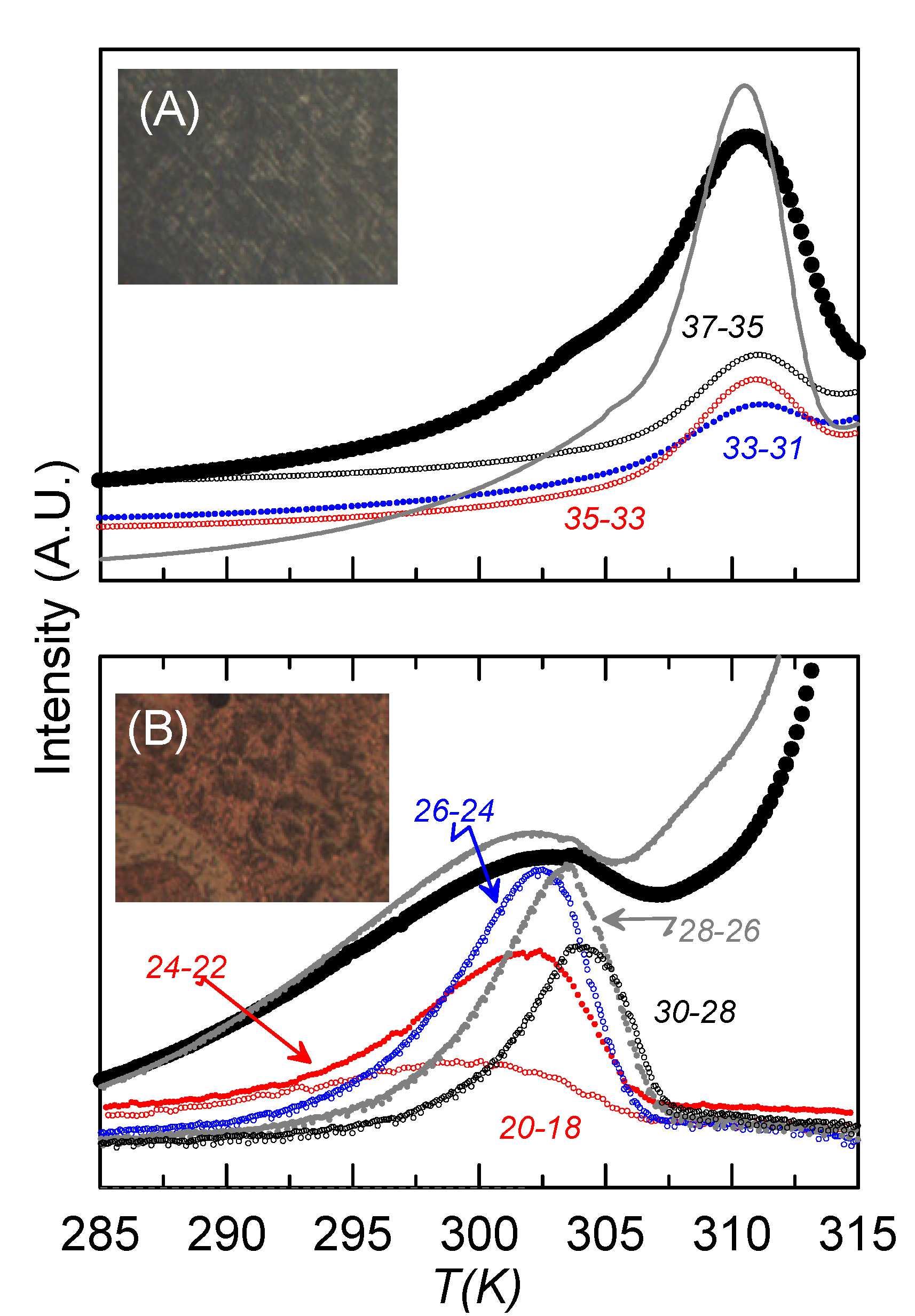
Together with the textures obtained from the microscope,
Figure 7 shows the complete (large circles) and some of the NIW-RMA experimental curves (small circles) of the depolarization current
vs. temperature for the sample with ρ
s = 0.23 g·cm
−3, for both homeotropic-like (
Figure 7A) and mixed (
Figure 7B) alignments. The complete curves obtained by TSDC can be associated to dielectric loss measurements at an extremely low frequency [
32], even below that corresponding to the glass transition (10 mHz). Confirming the results from dielectric spectroscopy, two main relaxations can be observed at well-defined temperatures, which differ in about 7 K, as happened in the dielectric measurements at the glass transition. The one at a lower temperature (302 K) should be the overlap of m
2 and m
1H, as it corresponds to higher frequencies at the same temperature. This mode is higher in strength when the sample is less homeotropic-like, which is coherent with the fact that m
2 should be residual in homeotropic alignments and the strength of m
1H at such low temperatures is very small. The other one (at 309 K), with a much higher strength when the sample is homeotropic-like, should be m
1L. The complete curves for the bulk sample are also present in
Figure 7 (grey lines), to show how the results are qualitatively similar for bulk and confined samples.
Figure 7.
TSDC curves vs. temperature for the sample ρs = 0.23 g·cm−3 for (A) homeotropic-like and (B) mixed alignments. Big black circles represent the “complete” curves. Small circles account for some of the NIW curves for each alignment. The name of each NIW curve is “Tp1-Tp2”. Textures for each alignment from the polarizing microscope are also shown. Grey lines account for the “complete” curves of the bulk under similar conditions.
A further confirmation of the good agreement between dielectric and TSDC results comes from the fitting of the TSDC relaxation modes (RMA analysis) to some phenomenological models from which the activation energies can be obtained. If a relaxation mechanism has first order kinetics, the calculated depolarization current can be obtained from the equation
where
P0 is the initial polarization of the sample,
τ(
T) is the relaxation time of the process and
κ is the heating rate. The relaxation time can be modeled through several empirical models. We use the Arrhenius equation
and the Narayanaswamy-Moynihan equations
where
E is the activation energy, τ
0 the preexponential factor and
T and
x (which is related to cooperativity) are empirical parameters.
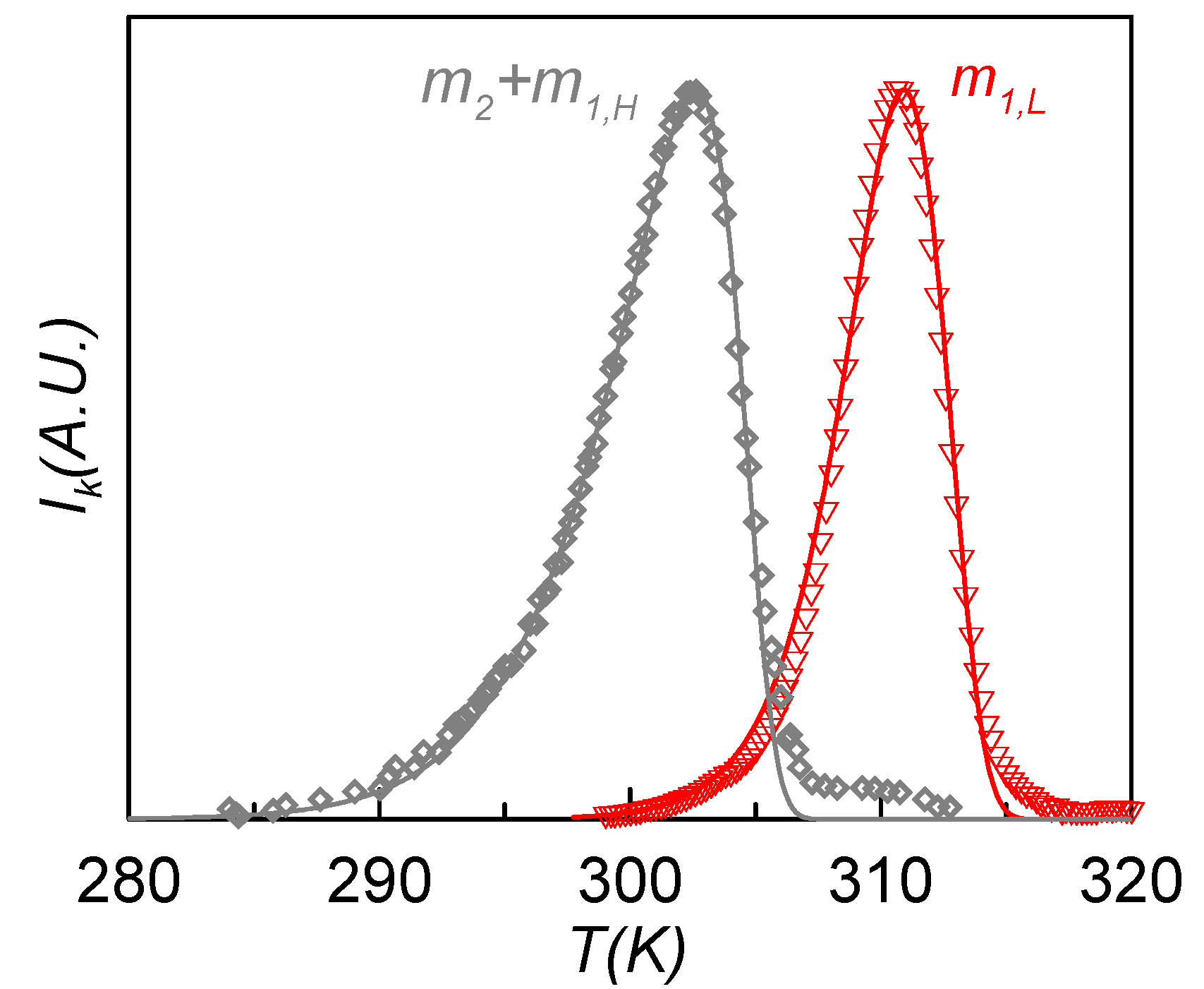
Figure 8 shows the experimental (symbols) and calculated (lines) TSDC spectra of the m
1L (red) and m
2 + m
1H (grey) relaxation modes obtained in the RMA analysis of the sample poled at
Tp1 = 308 K (12 MV·m
−1) and
Tp1 = 301 K (1.6 MV·m
−1), respectively. These curves correspond to the contributions of maximum depolarization response, and so they are the more representative of each relaxation mode. Each depolarization curve of the RMA analysis was fitted to Equation (3) using the Arrhenius and the Narayanaswamy-Moynihan models for the relaxation time dependence. The obtained results show that m
1L is best fitted with the Arrhenius equation, while for m
2 + m
1H the best results are obtained with the Narayanaswamy-Moynihan model. This behavior indicates that the m
2 + m
1H relaxation is more cooperative than the m
1L one, which agrees with the results obtained from dielectric measurements.
Figure 8.
Experimental (symbols) and calculated (lines) TSDC spectra of the m1L (red) and m2 + m1H (grey) relaxation modes obtained in the RMA analysis of the sample poled at Tp1 = 308 K (12 MV·m−1) and Tp1 = 301 K (1.6 MV·m−1).
Figure 8.
Experimental (symbols) and calculated (lines) TSDC spectra of the m1L (red) and m2 + m1H (grey) relaxation modes obtained in the RMA analysis of the sample poled at Tp1 = 308 K (12 MV·m−1) and Tp1 = 301 K (1.6 MV·m−1).
2.4. Specific Heat Evidence for Two Glass Transitions
Both dielectric spectroscopy and the RMA from TSDC measurements point to the existence of two glass transitions separated by a temperature gap of about 7 K. When analyzing the specific heat of
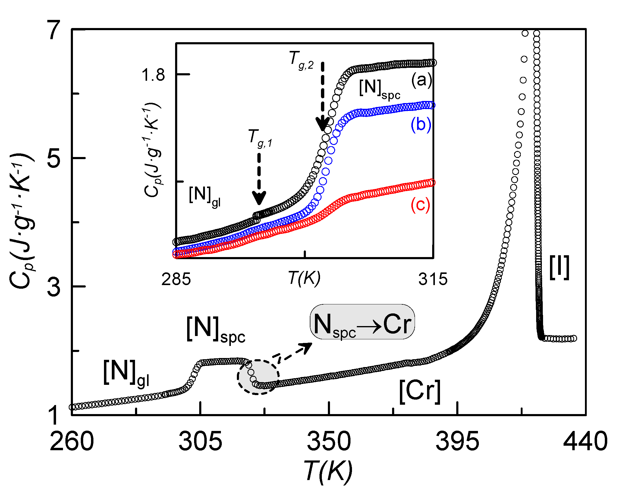
Figure 1, where the glass transition of one of the confined samples is shown after getting the N glassy state at different cooling rates, no apparent existence of two glass transitions is observed.
Figure 9 shows the specific heat on heating the sample ρ
s = 0.23 g·cm
−3 from 260 K after a fast cooling (20 K·min
−1). As it can be observed, the data for this sample are qualitatively similar to those shown in
Figure 2 for ρ
s = 0.16 g·cm
−3. Let us consider the inset of
Figure 9, where the jump in the specific heat is shown for the sample coming from several cooling rates. In the case denoted by (a), corresponding to a cooling rate of 20 K·min
−1, two consecutive glass transitions can be unambiguously observed about 7 K apart. In the other cases, (b) and (c), these two specific heat jumps cannot be clearly observed.
Figure 9.
Specific heat
vs. temperature for the sample of ρ
s = 0.23 g·cm
−3, heating up from 260 K after a fast cooling (20 K·min
−1). As it can be observed, the data for this sample are qualitatively similar to those shown in
Figure 2 for ρ
s = 0.16 g·cm
−3. The inset shows the jump in specific heat coming from several cooling rates: (a) 20 K·min
−1, (b) 15 K·min
−1, (c) 10 K·min
−1.
The first sight of
Figure 2 apparently leads to the same conclusion. In our opinion, the existence of two glass transition temperatures is independent of the concentration of γ-alumina nanoparticles. First of all, the TSDC spectra for bulk CBO11O.Py is qualitatively similar to that of the confined sample, as can be seen from
Figure 7. From specific heat measurements, the cooling rate to achieve the glassy state is a crucial parameter. For high enough concentrations of γ-alumina nanoparticles (ρ
s ≥ 0.23 g·cm
−3), the total vitrification of the N phase is believed to be obtained for cooling rates of 20 K·min
−1. For lower concentrations of nanoparticles, including the bulk, the highest cooling rate does not seem to be sufficient to avoid the coexistence of a small part of crystal with the nematic glassy state, making the observation of the two glass transition temperatures more difficult.
The different values in the specific heat capacity jumps can be explained as follows: As the pyrene group is considerably bulkier than the cyanobiphenyl one, the m1L mode requires more energy than both m2 and m1H. So, the jump in the specific heat is more pronounced in the glass transition at Tg2 (=TgPy).
There are some other systems in which two glass transitions have been found in the same phase [
35,
36,
37], but this is the first time, to the best of our knowledge, that two close glass transitions have been unambiguously identified in the same supercooled mesophase of any liquid crystal.


