1. Introduction
The compatibility approach [
1,
2,
3] focuses on calculating the relative current density
u which is defined as the ratio of electric and thermal fluxes,
. Note that
and
are vectors. The advantage of using the relative current density
is that the complex thermoelectric (TE) problem can be reduced to a one-dimensional heat flow problem. In particular, this approach can be used as a mathematical basis to analyze the local performance of TE material [
4,
5].
The total performance (efficiency
η and coefficient of performance
, respectively) of a thermogenerator (TEG) or Peltier cooler (TEC) element is obtained by summing up all local contributions in an integral sense as originally proposed by Harman and Honig [
6], see also [
4,
7]:
where we identify one kernel for integrals of both generator and cooler. The model is based on an ideal single element device (prismatic TE element of length
L and fixed boundary temperatures) without parasitic losses, for more information see [
4,
5]. Then, the device figure of merit is equal to the traditional material’s figure of merit,
, with the Seebeck coefficient (
α), electrical resistivity (
ρ), and thermal conductivity (
κ).
The Integrals (1) can be optimized with respect to the relative current
u. An optimized
u represents an optimal ratio between heat flux and electrical current density and hence a maximum performance value given in self-compatible elements by the compatibility factors
of a TEG, but
of a TEC, firstly introduced by Snyder [
1,
2]. Thus global maximization is traced back to local optimization [
8].
If we assume the ability to achieve full self-compatibility (considering the case of infinite staging) we can apply
and
to the Integrals (1), respectively, so that they take their maximal values with the optimal reduced efficiency
for both TEG and TEC [
9,
10]. Then, fully self-compatible performance parameters
and
are given by
where we identify expressions being monotone with
in the integrands. For the notation used we refer to [
4,
5].
We expressly emphasize that the Integrals (2) do not have extremal properties concerning the
value. Usually they are evaluated analytically for constraints
const. or
const., for details see the appendix of [
8]. In particular the latter case is easy to handle. We obtain with constant values
for the Integrals (2)
The question of how to get the best performance can only be answered if we put the constant
in relation to the TE material characterized by an experimental
. A proof for the relations
is given in [
4], if
is calculated as the average over temperature of a
monotonically increasing function ,
Equality holds if const. If is decreasing, however, the above inequalities in general do not hold. Hence, we look for an optimal where and , respectively, and , will be maximal. Since the integrals cannot be optimized for arbitrary we consider a constraint optimization problem including Condition (5). The solution enlightens the role of the constraint const. which is often used in practice.
2. Linear Functions k(T) = z(T)T
Before turning to the general problem, let us examine linear functions .
We define straight lines
by the formula
and boundary values
The goal is to estimate the optimal
which gives maximum performances
and
, respectively. Exemplarily,
Figure 1 shows the results for
and
for both TEG and TEC. Having found
, the optimal function
can be derived, see
Figure 2. Note that
is decreasing with temperature for TEG (leading to a small performance increase of about
for
), but the maximal coefficient of performance of a TEC is very close to
const. when considering straight lines
.
More generally, one can prove for straight lines: For both a TEG and TEC, the performance increases if we cross the function
const. from increasing straight lines to decreasing straight lines. For TEG the existence of a maximal performance value in the class of straight lines depends on
and on the quotient
. There is a maximum in efficiency if
is large enough and
is not too large. Otherwise, the performance
increases the stronger
is falling. We see this effect in our example, see left subfigure of
Figure 1: For
(solid curve) a clear maximum of
η appears at
. For a smaller
the maximum is not so manifest (dashed curve). This
is only a little bit larger than the critical value
for
, where a maximal performance value no longer exists. For
the dashed curve in
Figure 1, left side, would be monotonically increasing for all
.
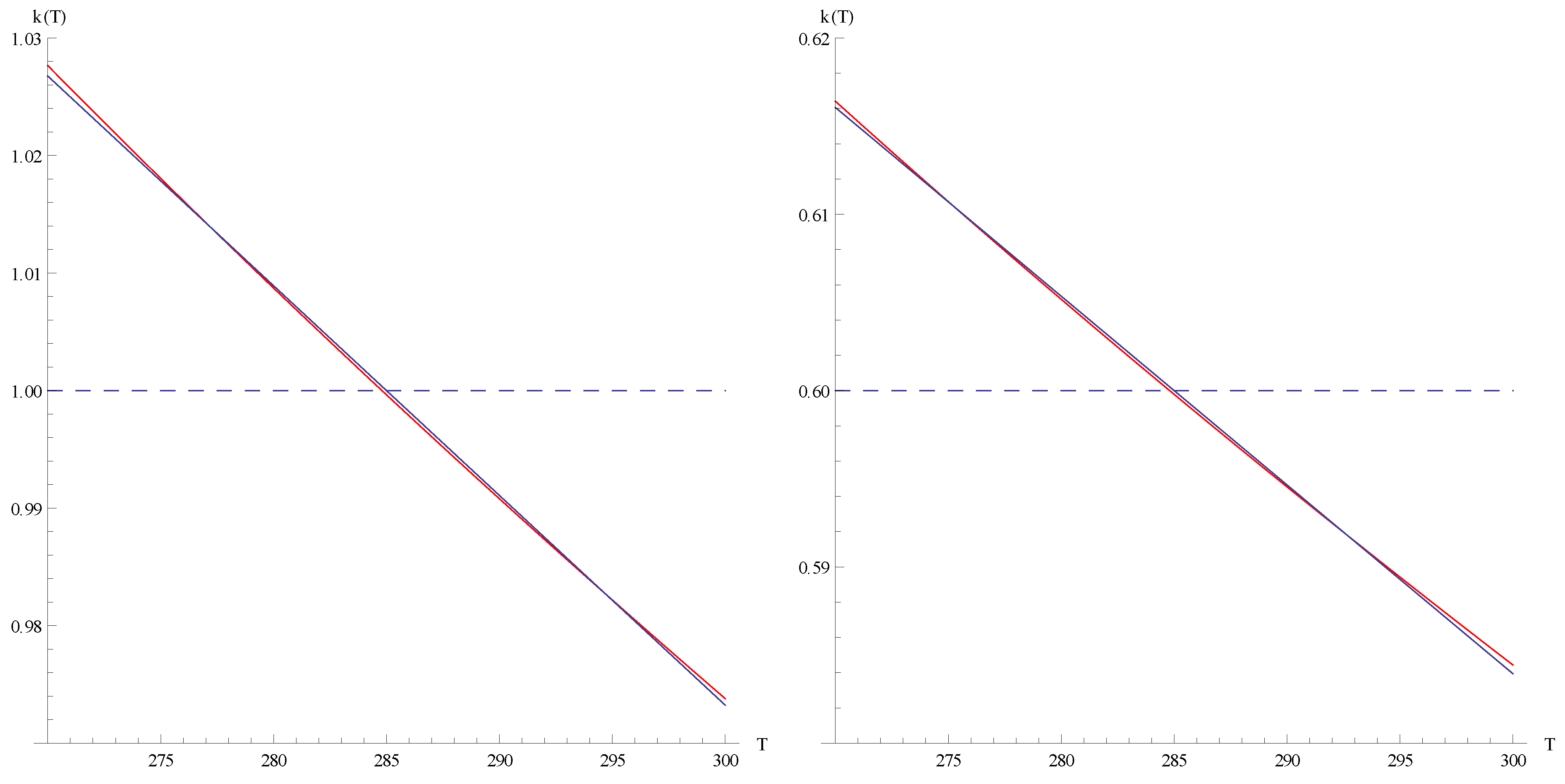
Figure 1.
Relative performance increase R as function of the parameter ξ: left: for TEG () for (solid curve, optimal efficiency at ) and (dashed curve, at , curve slowly decreasing for as long as ); right: for TEC () for (solid) and (dashed), optimal coefficient of performance at for both curves.
Figure 1.
Relative performance increase R as function of the parameter ξ: left: for TEG () for (solid curve, optimal efficiency at ) and (dashed curve, at , curve slowly decreasing for as long as ); right: for TEC () for (solid) and (dashed), optimal coefficient of performance at for both curves.
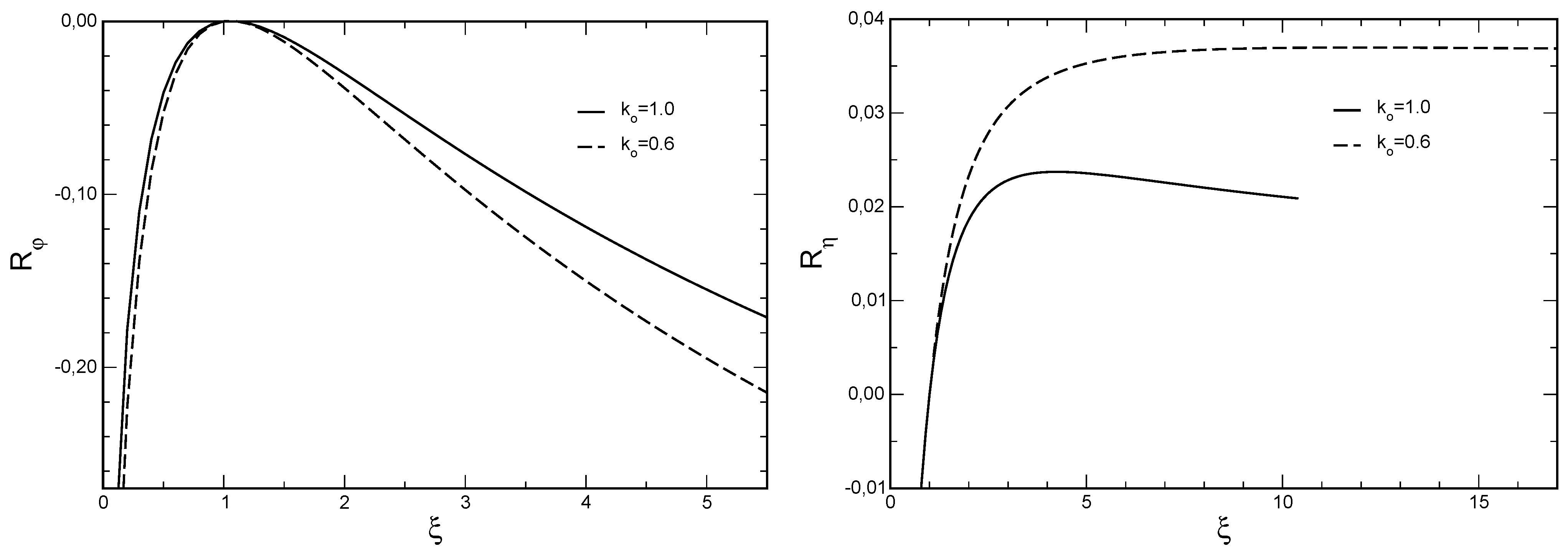
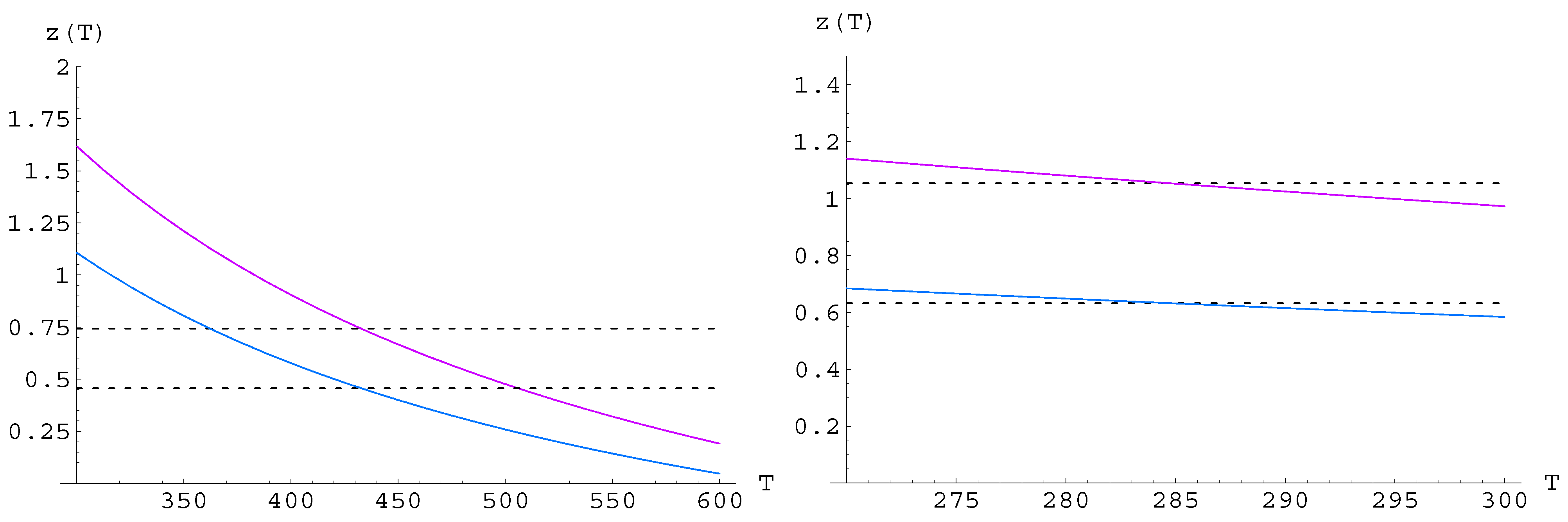
Figure 2.
Optimal straight line
plotted with the optimal parameter
derived from
Figure 1: left (TEG):
for
(purple) and
for
(blue); right (TEC):
(from
for
to
for
, with
for
and
).
Figure 2.
Optimal straight line
plotted with the optimal parameter
derived from
Figure 1: left (TEG):
for
(purple) and
for
(blue); right (TEC):
(from
for
to
for
, with
for
and
).
For a TEC we have a different situation. There is always a maximal coefficient of performance
in the class of straight lines
for some
(decreasing
k) independent of
and
. In general, however, this optimal value
is very close to
and in our
Figure 1 (right subfigure) it seems that this might be 1. Actually, the maximal value of
is attained at
and exceeds
by only
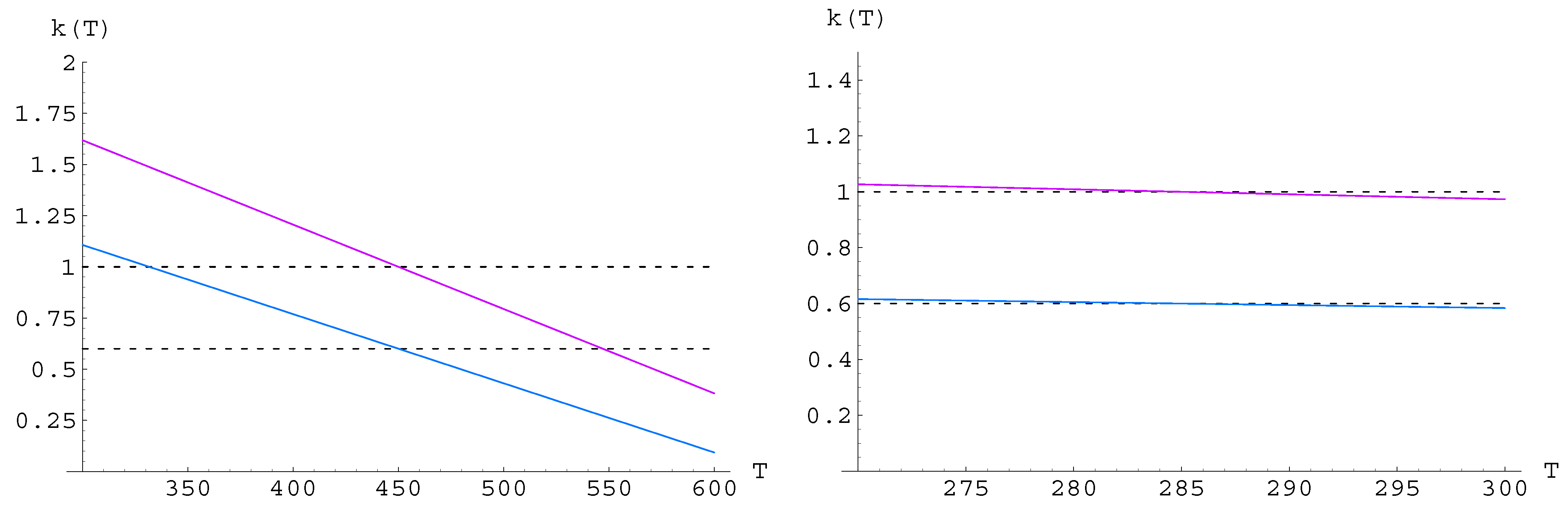
. From these results, the optimal figure of merit
can be calculated, see
Figure 2 and
Figure 3. The large effect for TEG (left) is obviously due to the fact that the temperature range of
for TEG is ten times larger than for TEC.
Figure 3.
Optimal figure of merit
; left TEG, right TEC (for boundary temperatures and colours see the legends of
Figure 1 and
Figure 2).
Figure 3.
Optimal figure of merit
; left TEG, right TEC (for boundary temperatures and colours see the legends of
Figure 1 and
Figure 2).
In the next section we derive a condition for the optimal profile . It turns out that this optimal function is not a straight line, but the situation is similar to the case of straight lines described above. The optimal function is decreasing again, and there is the same qualitative connection between and the existence of an optimal profile. Especially for a TEC, the restriction to straight lines will be a good approximation of the solution.
3. Isoperimetric Variational Problem
In this section we solve the two isoperimetric variational problems
with Constraint (5). The corresponding Lagrange functions (with Euler multiplicator
λ) are
and
respectively, where
and
. Hence, Euler’s equation reduces to
together with Condition (5). Differentiating Equation (
10a) and Equation (
10b) we obtain the following necessary relation for the optimal profile
to Problem (9),(5).
Theorem 1. Let or be an optimal function that maximizes the Integral (9a) or minimizes the Integral (9b), respectively, under Restriction (5). Then it fulfills the Equationswhere is a real constant depending on by means of In order to calculate the optimal solution
we have to solve the System (11), (12). Substituting
, Equations (11) simplify to
Since
we look for solutions
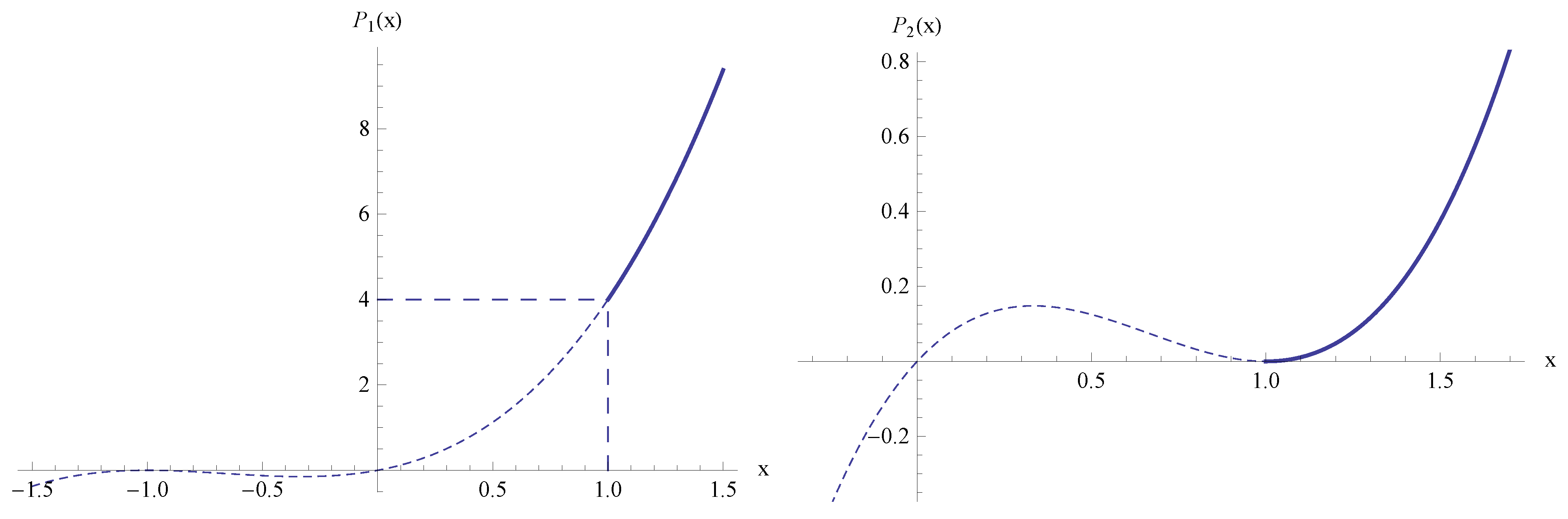
of Equations (13). From the graph of the polynomials
and
(see
Figure 4) we find that for fixed
the first Equation of (13) has exactly one real solution
if
. This implies the restriction
. The second Equation of (13) has exactly one real solution
for all
.
Figure 4.
Graph of polynomials and , see Equation (13).
Figure 4.
Graph of polynomials and , see Equation (13).
Then, resubstituting
x by
for fixed
μ with
, we obtain a unique positive solution of Equation (11a)
An analogue formula holds for the unique nonnegative solution of Equation (11b). To calculate the Representation (
14) an algebra tool (e.g., M
athematica) can be helpful.
It remains to determine the constant
μ. We have to choose it in a way that
from Equation (
14) fulfills Condition (12). The question whether we can find such a
μ is answered by the following theorem:
Theorem 2. - (i)
In case of a TEG there is a constant such that the following holds: If there exists a unique such that the function defined by Equation (14) fulfills Equation (11a) as well as Condition (12). Hence, . The corresponding is nonnegative on the interval , strictly monotonically decreasing and convex. If there is no constant μ such that the corresponding solution of Equation (11a) is nonnegative for every and fulfills Equation (12). In this case there is no optimal profile. - (ii)
In case of a TEC for every there exist a unique and a unique function which solve Equations (11b) and (12). The corresponding is nonnegative, strictly monotonically decreasing and convex.
Proof. - (i)
Let
be the (unique) solution of Equation (11a) for fixed
given by Equation (
14). We rewrite Equation (11a) by
and observe that the right hand side is strictly monotonically decreasing w.r.t.
T for every fixed
. Hence,
is a strictly decreasing function as well. This yields the nonnegativity of
if
which is fulfilled if
Therefore, we have the condition
for the nonnegativity of
for all
. We define now
and
. By the same argument as above we obtain from Equation (
15)
if
for every fixed
T. Consequently,
if
,
i.e.,
is strictly monotonically increasing. Moreover,
is a continuous function of
μ. This implies for every
the existence of a unique value
such that
, hence Equation (
12). For
there is no
such that
. Therefore there is no nonnegative function
which fulfills Equation (11a) and (12), which means that there is no extremal solution for the variational Problem (9a) with Constraint (5).
- (ii)
By the discussion above it is obvious that in the case of a TEC there is a unique and nonnegative solution
of Equation (11b) for every fixed
. The representation
of Equation (11b) yields that
is strictly monotonically decreasing with respect to
T and, moreover, that
increases for fixed
T if
μ increases. This implies the strict monotonicity of
. Furthermore, as illustrated in
Figure 4, if
μ decreases to zero then
decreases to zero (since
), hence
. Consequently, for every
there is a unique
such that the solution
of Equation (11b) fulfills the condition
,
i.e., it is the optimal solution of Equations (9b) and (5).
The proof of convexity of the optimal functions
is given in the appendix. ☐
Remark 1. - 1.
The observations in Section 2 on linear functions reflect the general result. Certain monotonically decreasing straight lines yield a better performance than the increasing ones. Moreover, as discussed in Section 2, also in the case of linear functions there is a critical value of for TEG, where we have no optimal linear function below of it. For a TEC such a critical does not occur. There we have an optimal performance in the class of linear function for every . - 2.
It is obvious that also will be strictly monotonically decreasing since has this property. Even more, will be a convex function. This can be justified by the following calculation using strict convexity of :Since for all T this can only be fulfilled if which means convexity.
In order to calculate the optimal TEG or TEC profile for given
, we now have to determine the constant
μ such that the solution
of Equation (11) satisfies Condition (12). Since we cannot evaluate the integral of a function like Equation (
14) explicitly, we have to use numerical methods to solve the equation
for
μ. Due to the strict monotonicity of
, a standard numerical solver will work.
Now we compare the best linear functions from
Section 2 with the optimal profile corresponding to Theorem 2. Again we choose
and
for a TEG and a TEC, respectively. We start with a TEG with
and
like in
Section 2.
We compare the corresponding values of the efficiency
for the three cases that
is a constant,
is the best linear function of
Section 2 and
is the global maximum of the variational Problem (9a),(5), see
Table 1:
Table 1.
Self-compatible efficiency of a TEG with and .
Table 1.
Self-compatible efficiency of a TEG with and .
| TEG | | |
|---|
| | | |
|---|
| constant function | 0.112126 | 1.00000 | 0.077873 | 1.00000 |
| linear function | 0.114786 | 1.02372 | 0.080752 | 1.03697 |
| optimal function | 0.114855 | 1.02434 | 0.080829 | 1.03796 |
Both from the above table and
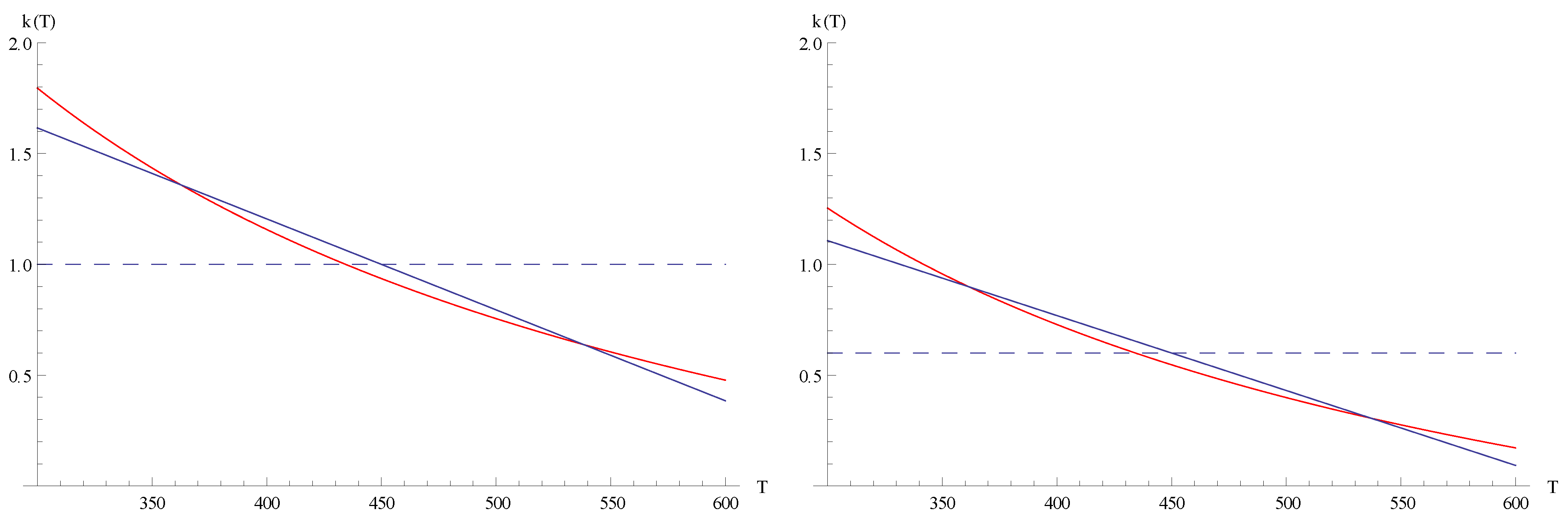
Figure 5 we see that the best straight line is a good approximation for the optimal profile. The optimal function
, due to Theorem 2, yields only a minimal increase in performance compared with the best linear function. This effect becomes even more apparent in the case of TEC which will be considered now (see
Figure 6). Like in
Section 2 we choose again
and
.
Figure 5.
Optimal functions
(red) compared with the best straight line
(blue) from
Figure 2 plotted with the optimal parameter
derived from
Figure 1. left:
for
; right:
for
.
Figure 5.
Optimal functions
(red) compared with the best straight line
(blue) from
Figure 2 plotted with the optimal parameter
derived from
Figure 1. left:
for
; right:
for
.
Figure 6.
Optimal monotonic functions
(red) compared with the best straight line
(blue) from
Figure 2 plotted with the optimal parameter
derived from
Figure 1. left:
; right:
. Please note the scaling of the y-axis.
Figure 6.
Optimal monotonic functions
(red) compared with the best straight line
(blue) from
Figure 2 plotted with the optimal parameter
derived from
Figure 1. left:
; right:
. Please note the scaling of the y-axis.
We observe that there is almost no difference between the best linear function and the optimal profile
which can be distinguished only thanks to the different scaling of the axes. Moreover, the scaling should not hide the fact that both functions nearly coincide with the constant
. Again we compare the maximal values of the coefficient of performance
for the three cases that
is a constant,
is the best linear function of
Section 2 and
is the global minimum of the variational Problem (9b),(5), respectively (
Table 2):
Table 2.
Self-compatible coeff. of performance of a TEC with and .
Table 2.
Self-compatible coeff. of performance of a TEC with and .
| TEC | | |
|---|
| | | |
|---|
| constant function | 1.17929125 | 1.0000000 | 0.68419337 | 1.0000000 |
| linear function | 1.17955485 | 1.0002235 | 0.68438545 | 1.0002803 |
| optimal function | 1.17955497 | 1.0002236 | 0.68438554 | 1.0002804 |
Here we see that for a TEC the constant function is a good choice, since there is only an insignificant increase of for the optimal function .
4. Discussion and Conclusions
The material’s figure of merit
z gathers as a primary parameter the different transport coefficients of thermoelectrics, leading to an efficient classification of the various TE materials. The dimensionless
in turn appears in a variety of thermodynamic expressions [
11]. At a first glance the presence of the temperature in the expression of the dimensionless figure of merit may be strange since
T is not a material property, but an intensive parameter which partly defines the working conditions. Nevertheless, one should notice that, in terms of thermodynamic optimization, the material properties are nothing without considering the available exergy of the working system, for more information see [
5,
11]. The figure of merit is clearly the central term for TE material engineering.
A general rule is that if a material is good (high
) then it is good in both TEG and cooler applications. However, the question is whether the constraint
const. can be considered as a local condition for an optimal material. The counter argument usually advanced is that the Seebeck coefficient
and the electric conductivity
have opposite shapes, which has given rise to the hope that a down-opened parabola
(resp.
) could be close to the optimal condition. This hope is not fulfilled when considering the problem from a mathematical point of view. In the performance integrals,
is representing an internal degree of freedom that must be fixed by an upper limit or similar constraint in order to prevent that global performance diverges. Doing so, a constraint optimization problem for the thermoelectric figure of merit has been formulated and solved. As the result we obtain convex, optimal functions
, slightly falling with temperature, for both TEG and TEC. It is well-known that curves
falling with temperature are practically not usable for most materials. However, it has turned out that the optimal function
is almost a constant
for a TEC and close to this constant function for a TEG, respectively (see
Table 1 and
Table 2). This fact underlines the importance of the constraint
const. which is often used in practice; usually this constraint can only be reached approximately.


