
Fatigue Tests and Analysis on Welded Joints of Weathering Steel

Abstract
:1. Introduction
2. Materials, Methods and Experiments
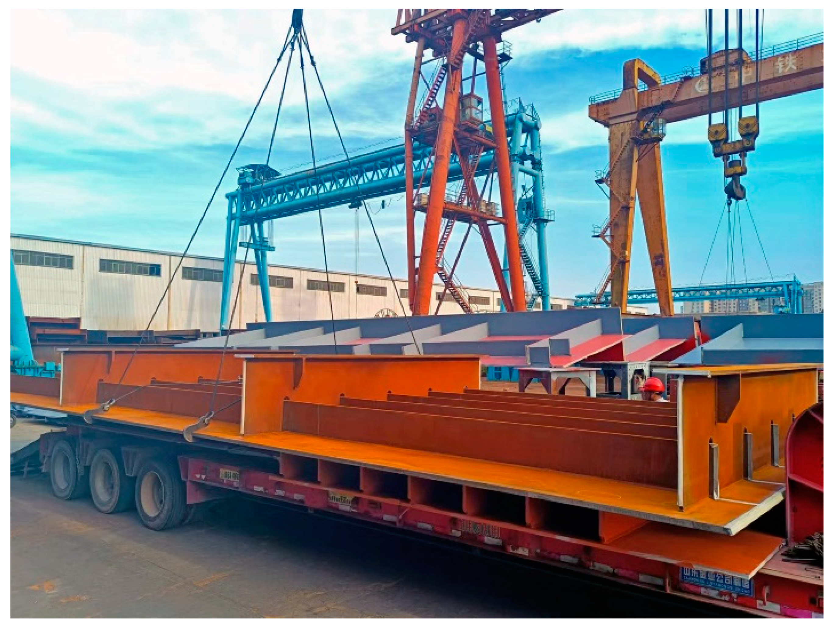
2.1. Specimens
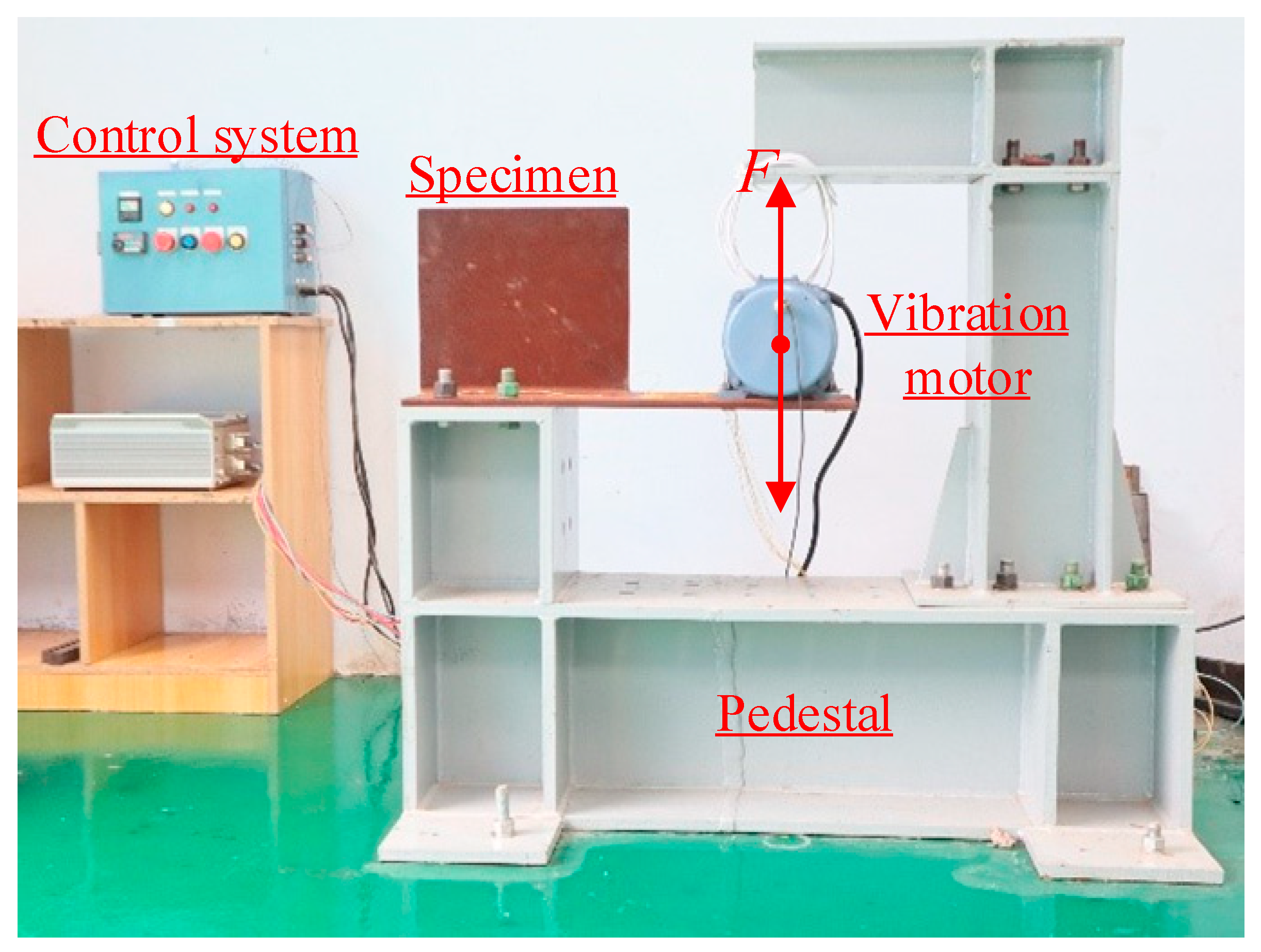
2.2. Test Setup
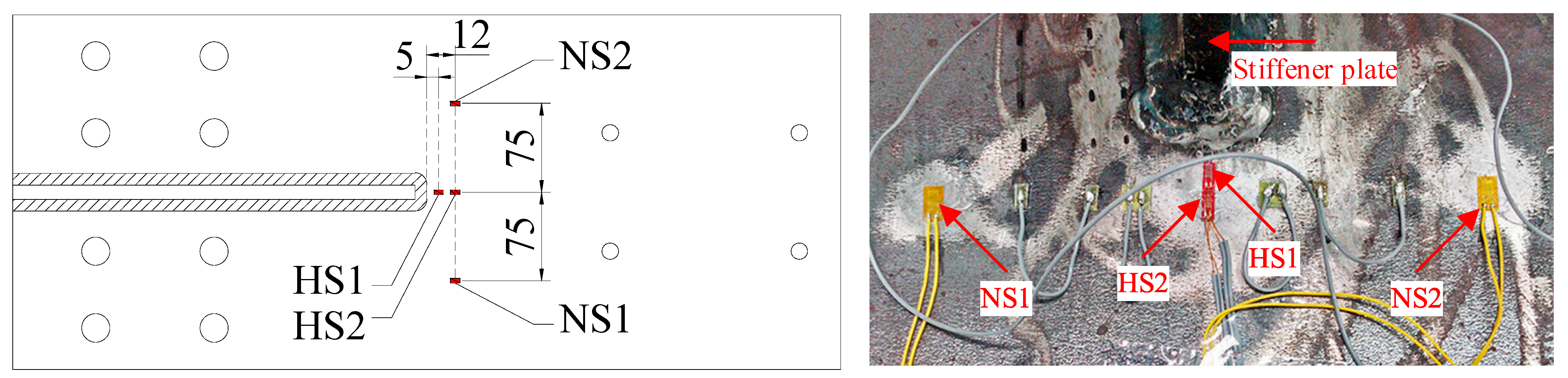
2.3. Instrumentation
2.4. Fatigue Crack Measurement
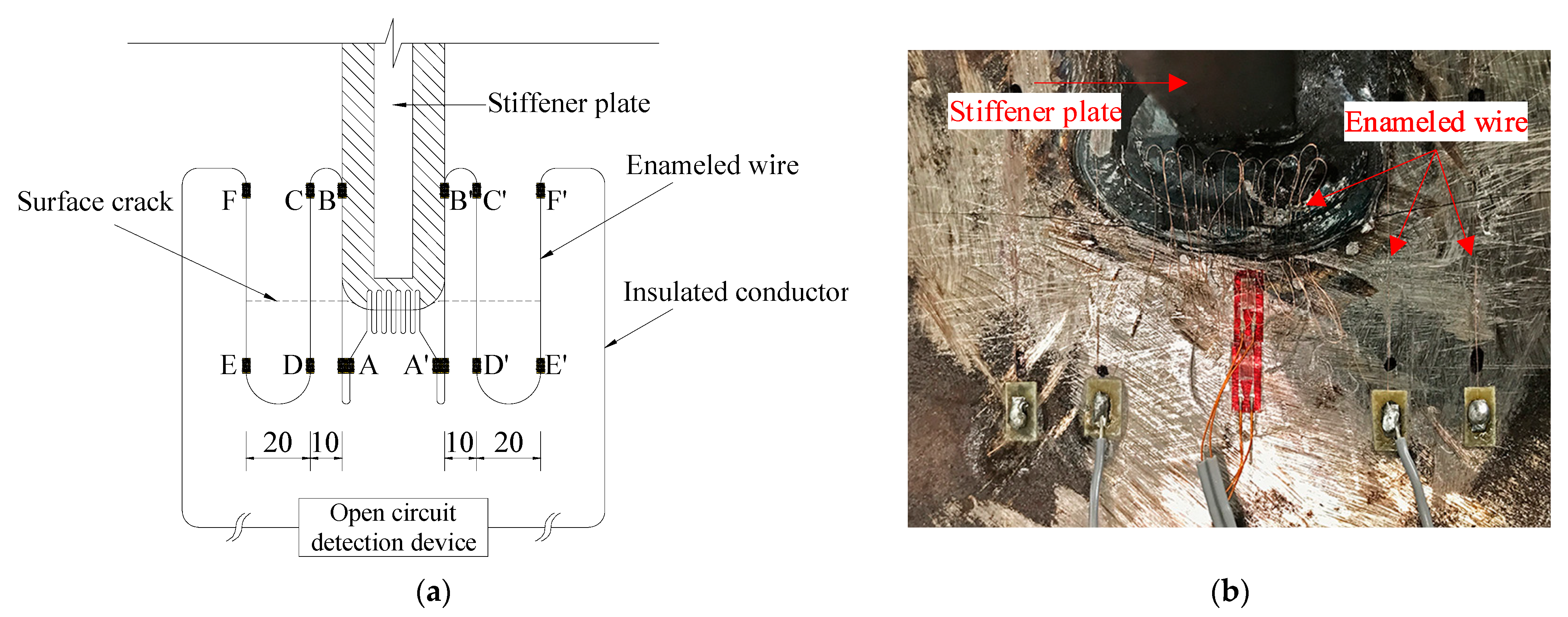
2.4.1. Surface Crack Monitoring
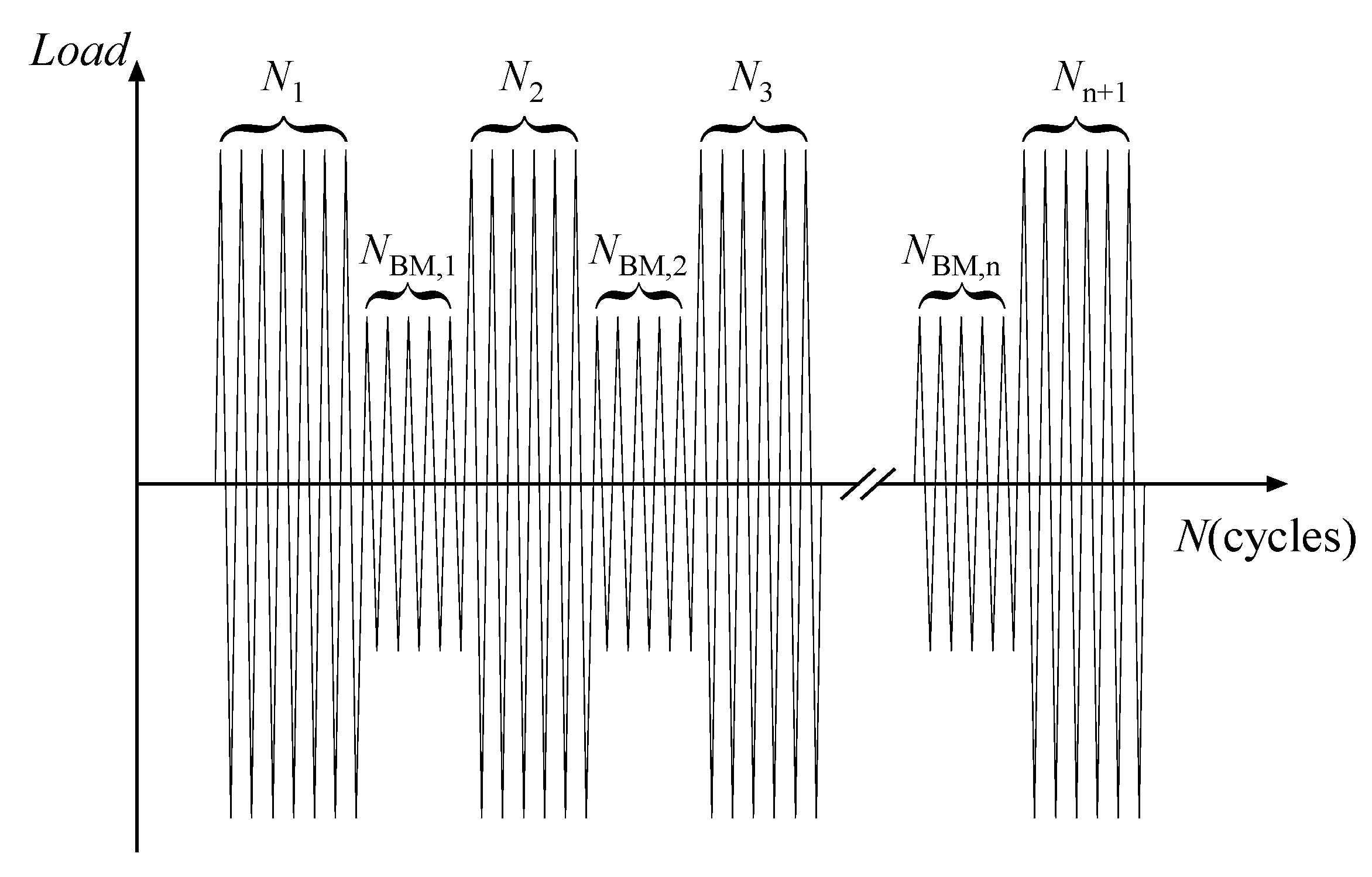
2.4.2. Beach Mark Testing
3. Test Results
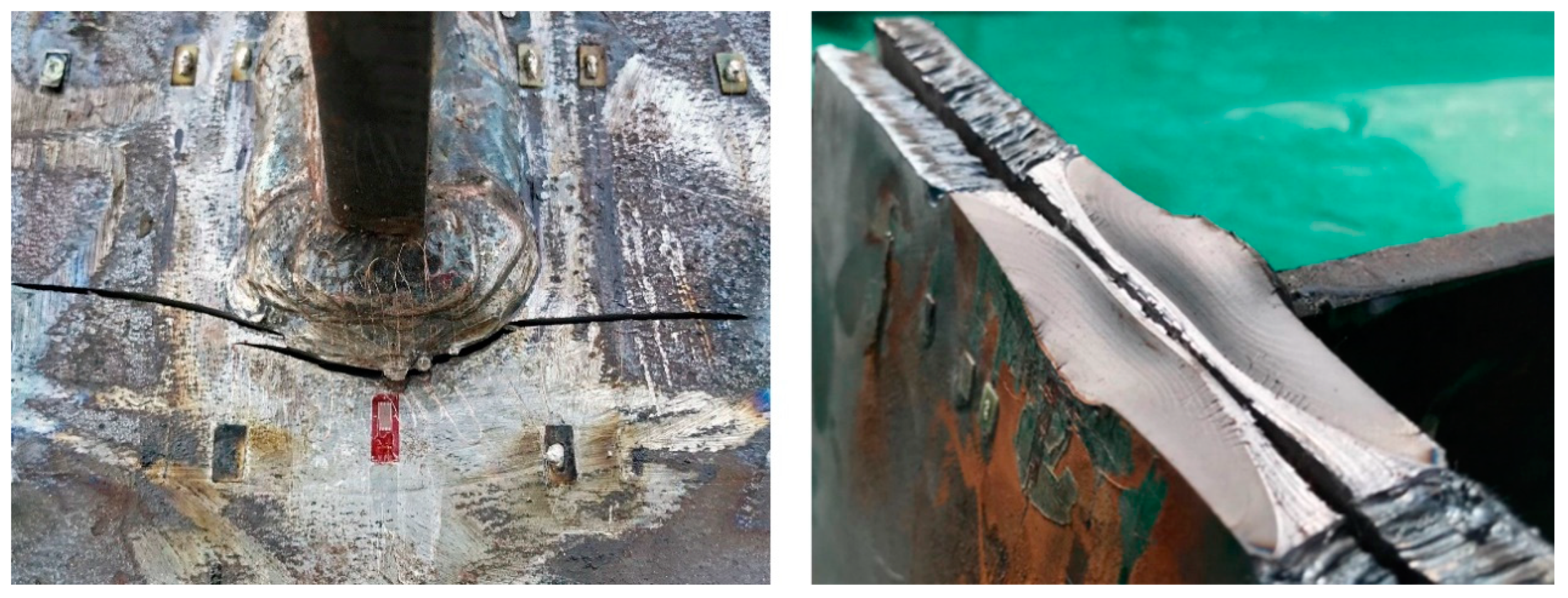
3.1. Failure Mode
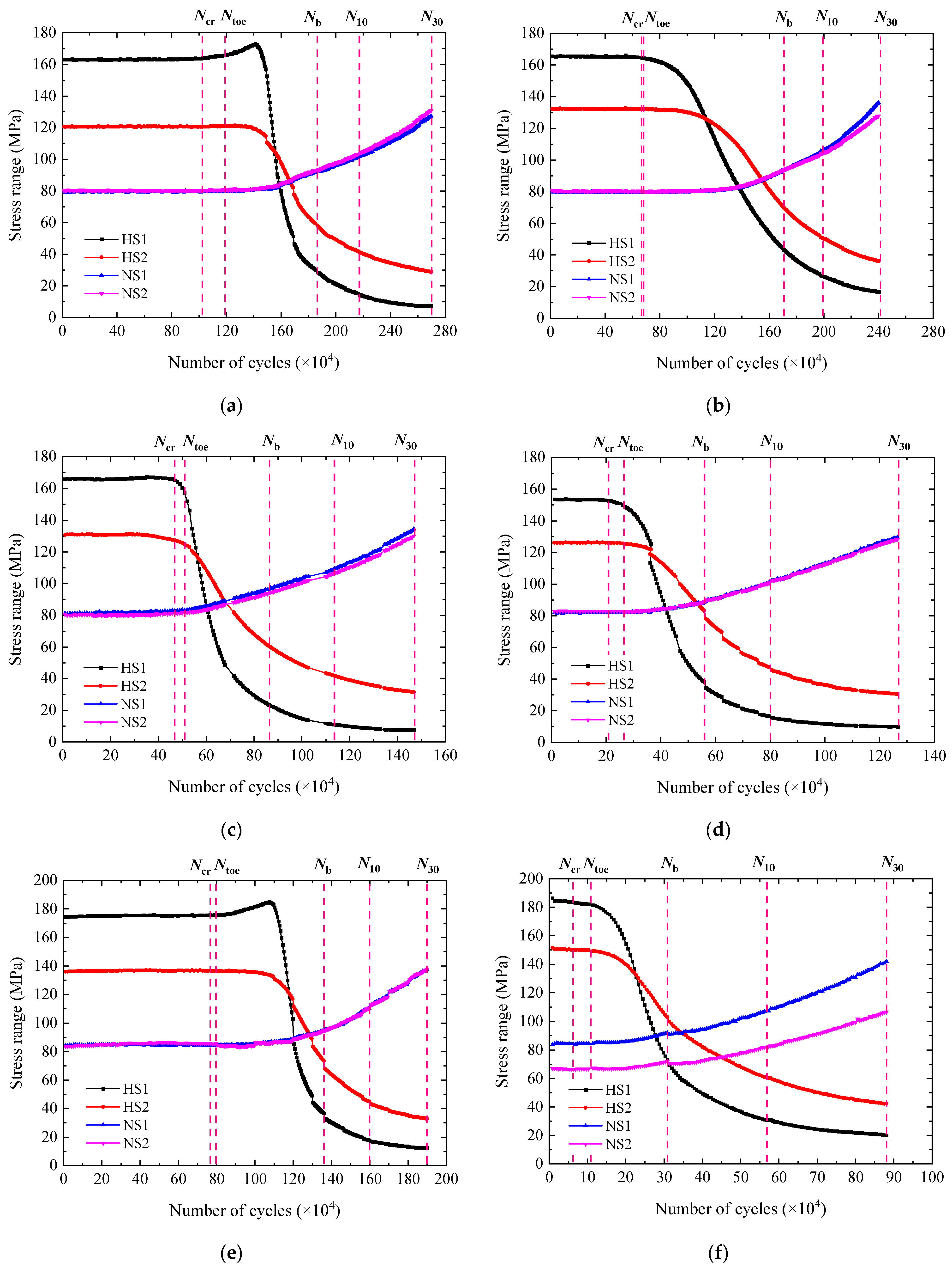
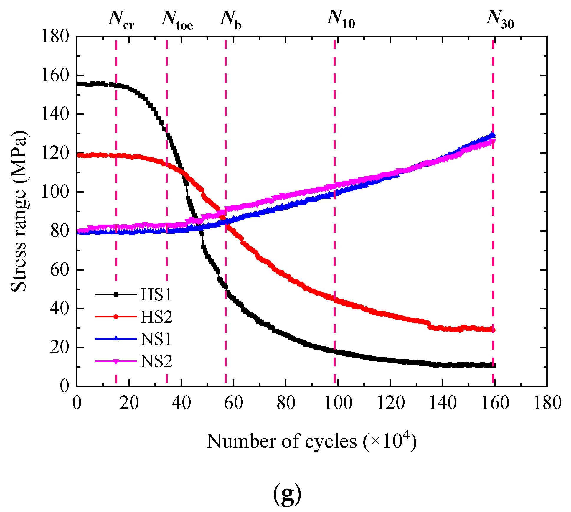
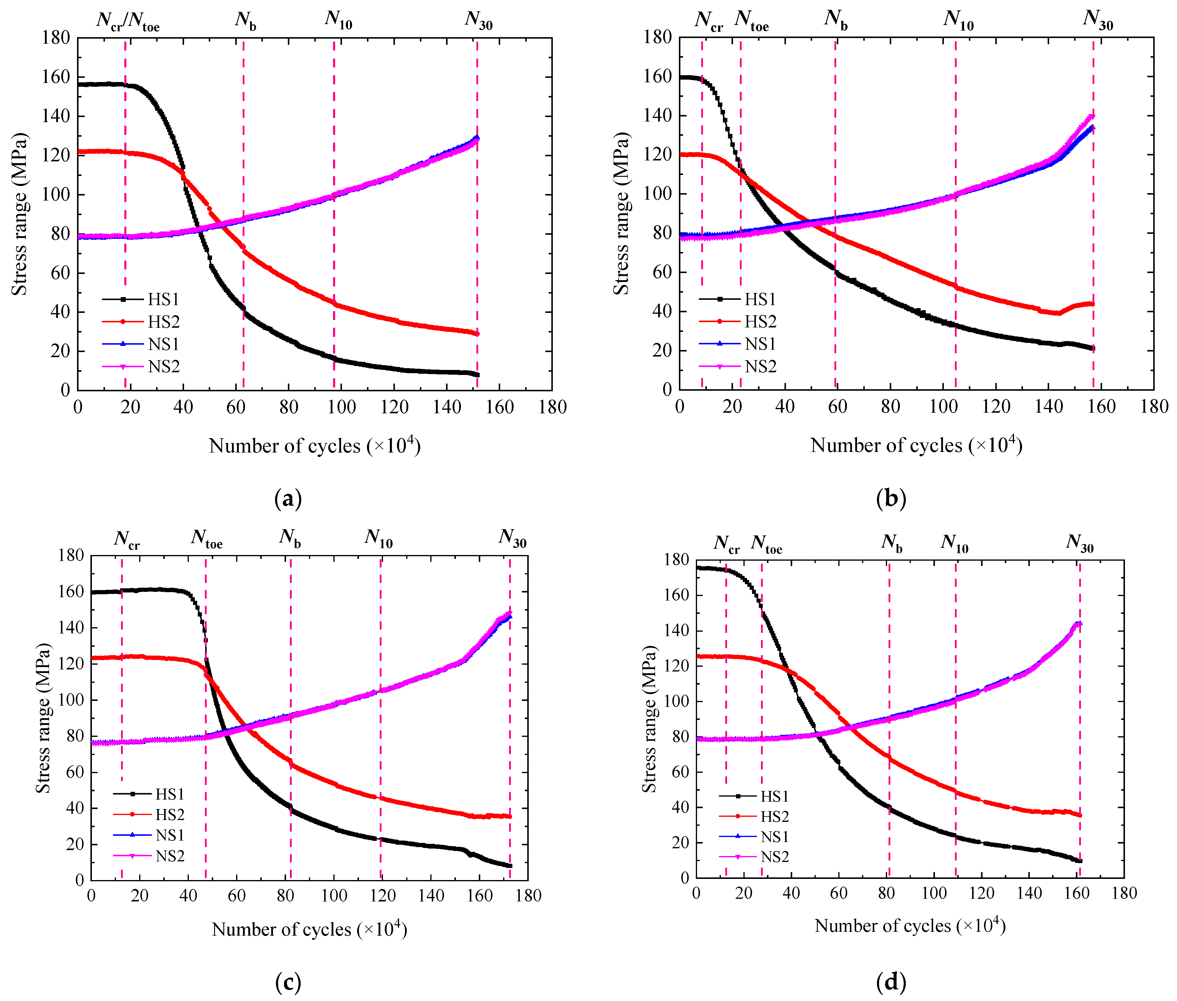
3.2. Stress Range
3.3. Fatigue Life
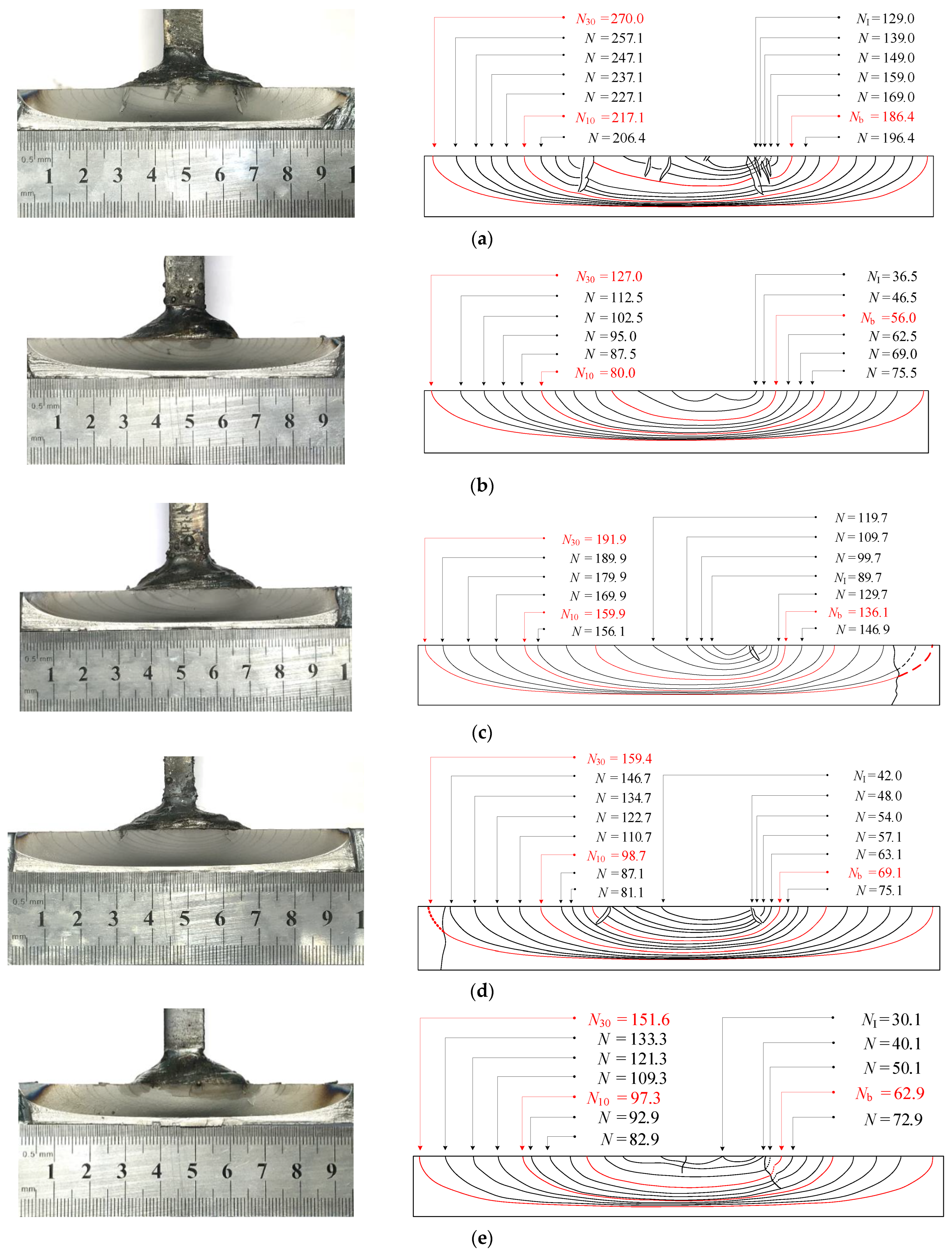
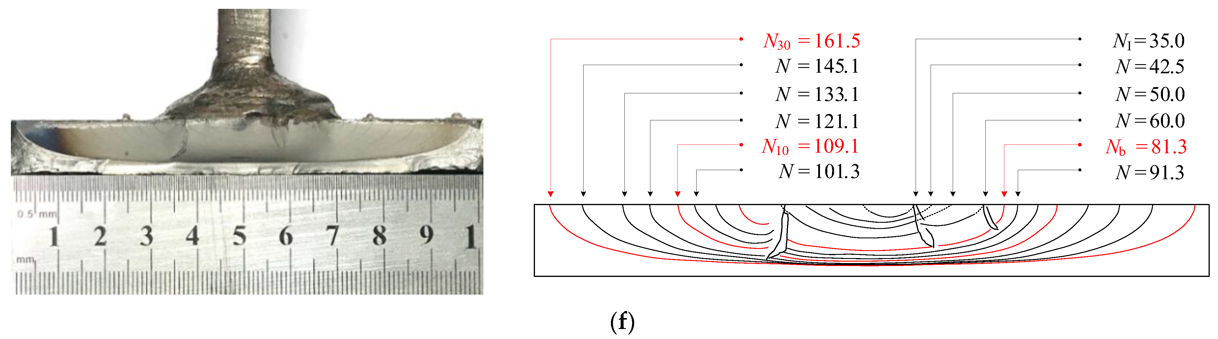
3.4. Fatigue Crack Propagation Characteristics
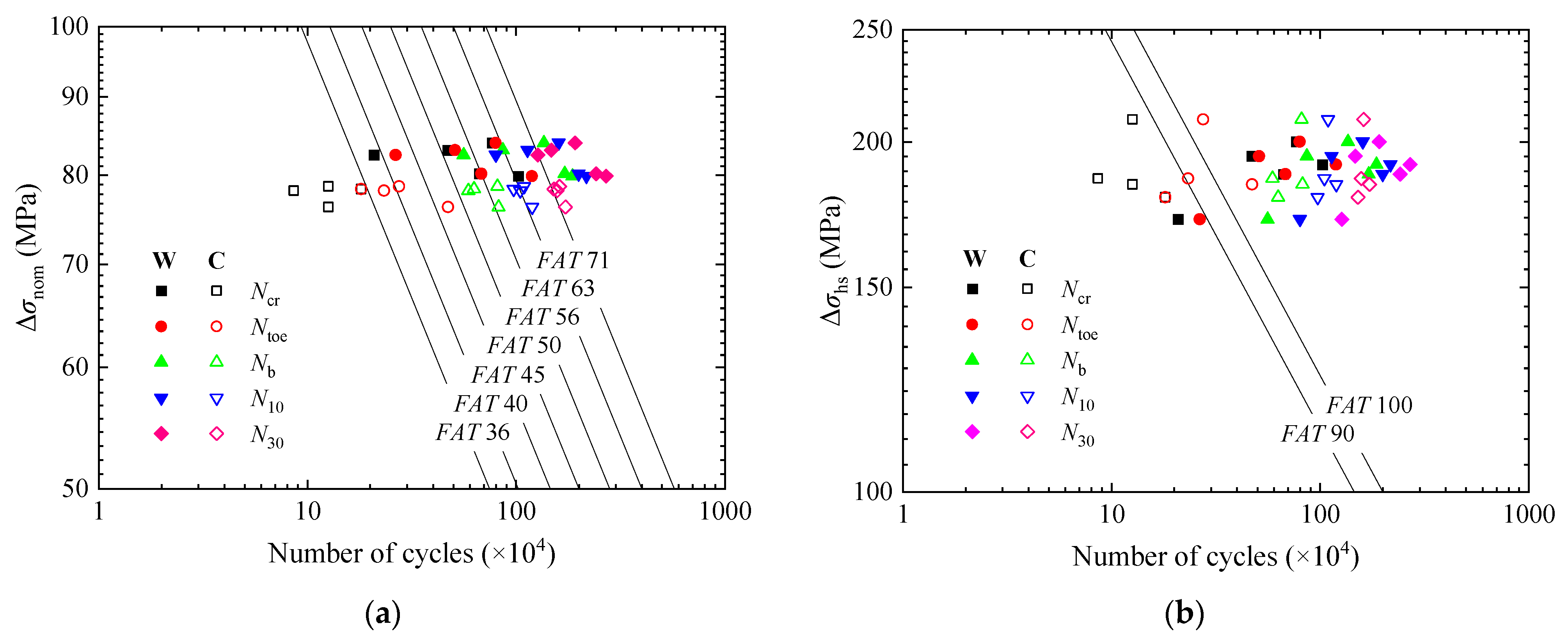
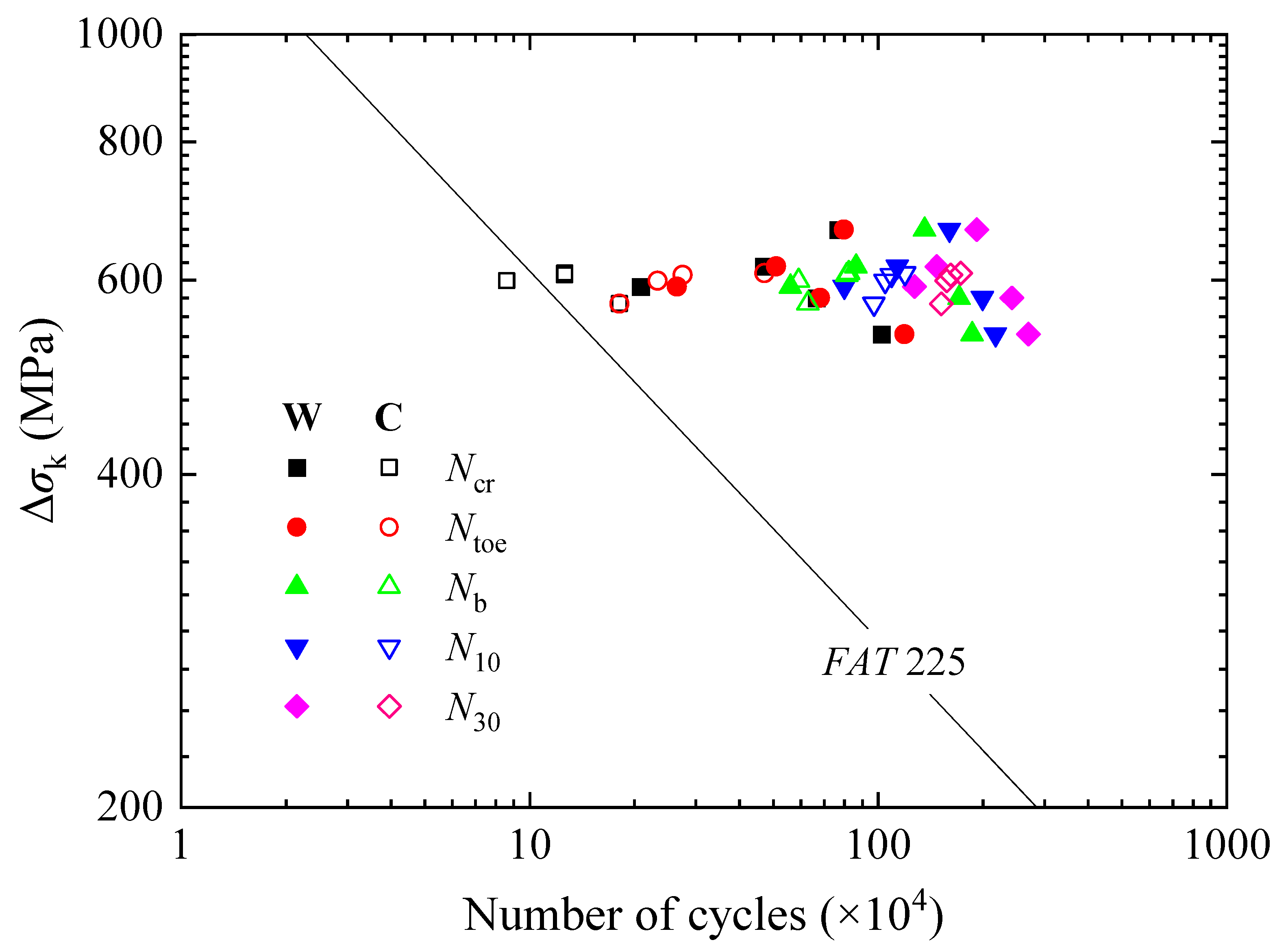
4. Fatigue Strength Evaluation Based on S-N Curves
4.1. Nominal Stress and Hot Spot Stress Approaches
4.2. Effective Notch Stress Approach
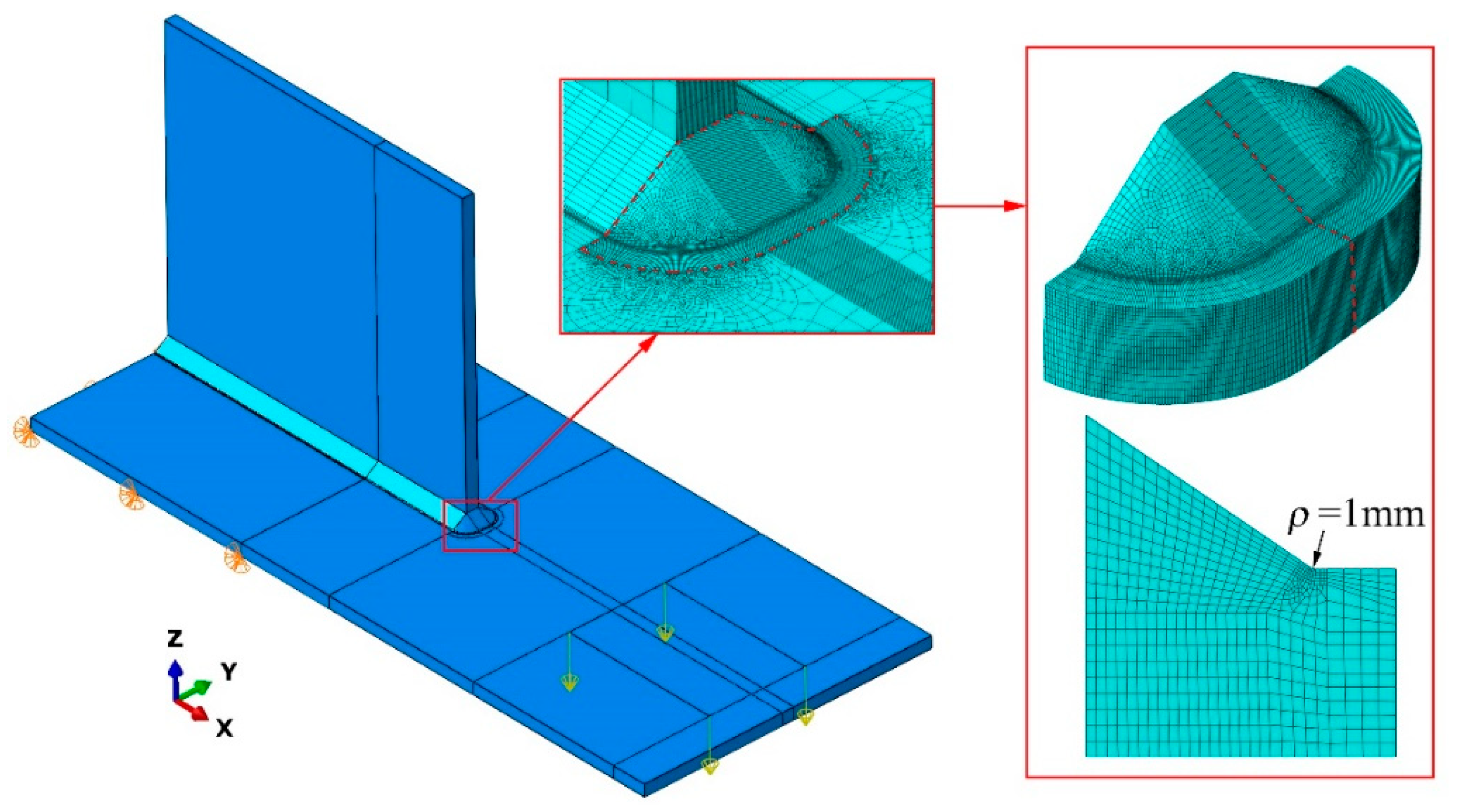
4.2.1. Finite Element Method Modeling
4.2.2. Results and Analysis
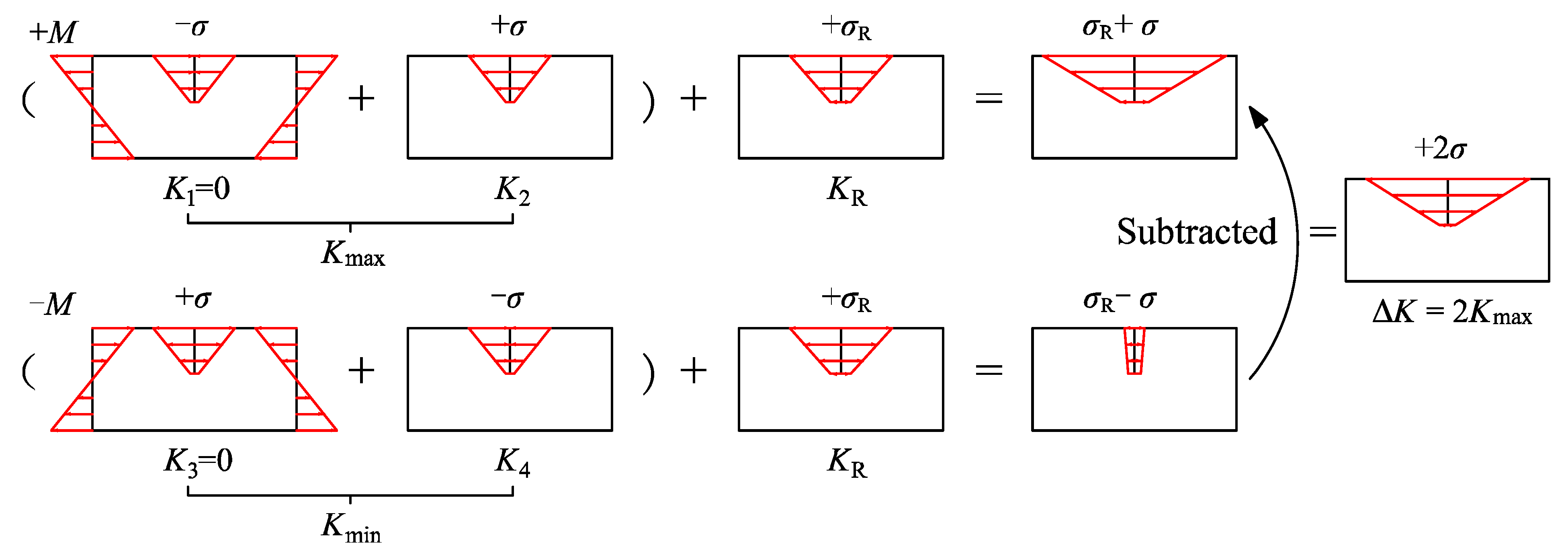
5. Fatigue Crack Propagation Analysis by LEFM
5.1. Extended Finite Element Method Modeling
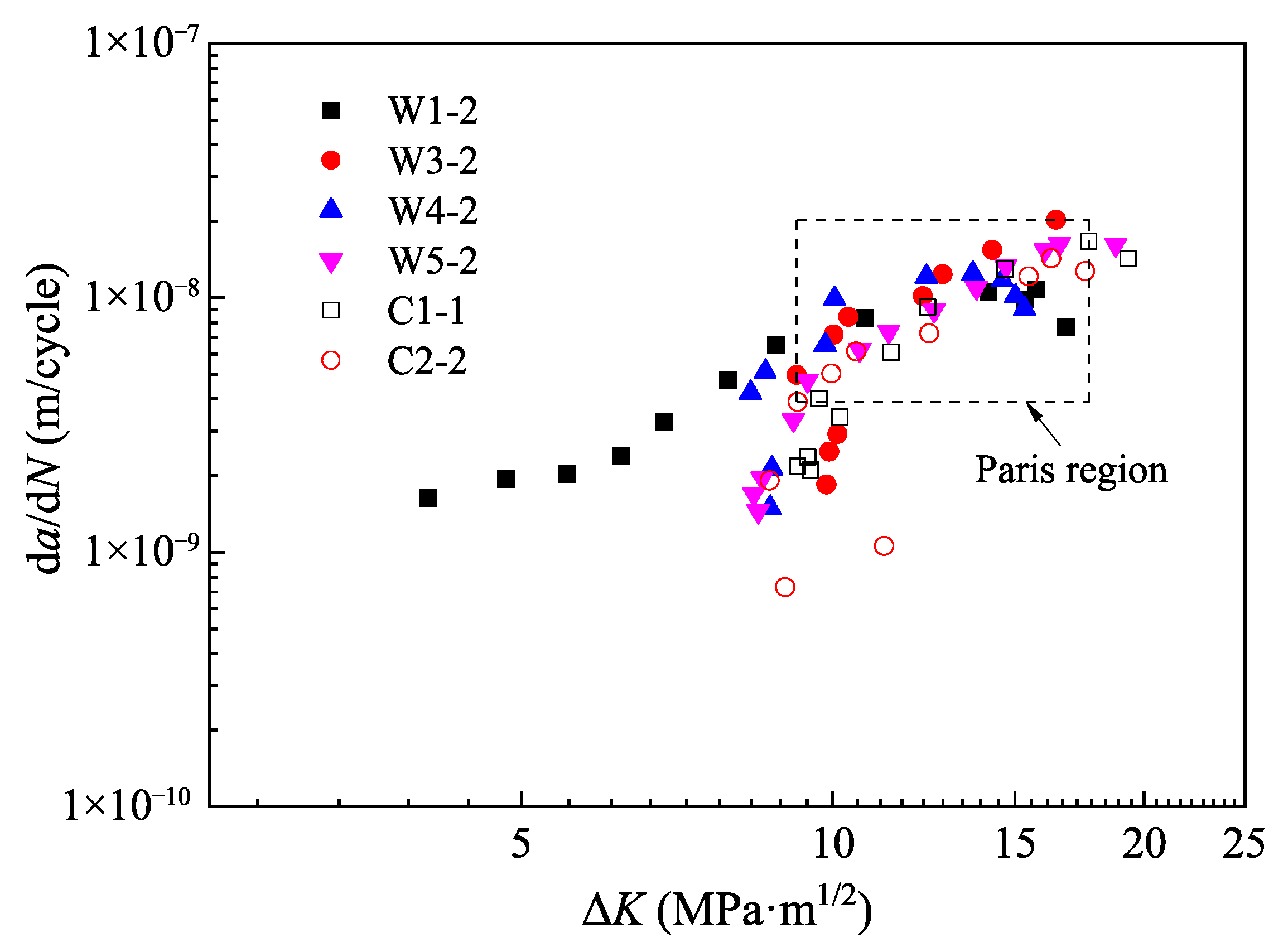
5.2. Fatigue Crack Propagation Rates
5.3. Material Constants for LEFM
6. Conclusions
- The fatigue tests of vertical web stiffener to deck plate welded joints showed that the fatigue crack was initiated from the end weld toe of the deck plate accompanied by multiple crack nuclei, and subsequently propagated both along the thickness of the deck plate and in the direction perpendicular to the stiffener plate. Finally, it almost penetrated through the deck plate.
- The fatigue crack initiation and propagation life of WS Q345qNH specimens was longer than that of CS Q345q specimens. The fatigue crack propagation life of WS Q345qNH specimens was longer than that of WS Q420qNH specimens, but the initiation life bore little relationship to the yield strength.
- Increasing the thickness of the stiffener plate effectively delayed fatigue crack initiation and slowed down its propagation. Compared with fillet welds, full penetration welds extended the fatigue crack propagation life, but no significant improvement was implied for the initiation life.
- The state where the crack reached the edges of the weld was taken as fatigue failure. The WS and CS specimens could be classified as having the same fatigue strengths by the nominal stress, hot spot stress, and effective notch stress approaches, which were FAT 50, FAT 100, and FAT 225, respectively. Meanwhile, their material constants for LEFM were relatively close to each other. The values of the material constant m for the specimens were slightly smaller than those of the recommendations by IIW, BS 7910, and JSSC, but the values of the material constant C were nearly the same. However, the beach marks are not accurate enough to track the early crack initiation in welded joints of WS and CS. New methods still need to be investigated to measure fatigue cracks during the early crack initiation.
Author Contributions
Funding
Institutional Review Board Statement
Data Availability Statement
Acknowledgments
Conflicts of Interest
References
- Morcillo, M.; Díaz, I.; Chico, B.; Cano, H.; de la Fuente, D. Weathering steels: From empirical development to scientific design. A review. Corros. Sci. 2014, 83, 6–31. [Google Scholar] [CrossRef] [Green Version]
- Qian, Y.; Ma, C.; Niu, D.; Xu, J.; Li, M. Influence of alloyed chromium on the atmospheric corrosion resistance of weathering steels. Corros. Sci. 2013, 74, 424–429. [Google Scholar] [CrossRef]
- Tewary, N.; Kundu, A.; Nandi, R.; Saha, J.; Ghosh, S. Microstructural characterisation and corrosion performance of old railway girder bridge steel and modern weathering structural steel. Corros. Sci. 2016, 113, 57–63. [Google Scholar] [CrossRef]
- Zong, Y.; Liu, C.-M. Microstructure, Mechanical Properties, and Corrosion Behavior of Ultra-Low Carbon Bainite Steel with Different Niobium Content. Materials 2021, 14, 311. [Google Scholar] [CrossRef]
- Chen, H.; Grondin, G.Y.; Driver, R. Characterization of fatigue properties of ASTM A709 high performance steel. J. Constr. Steel Res. 2007, 63, 838–848. [Google Scholar] [CrossRef]
- Su, H.; Wang, J.; Du, J. Experimental and numerical study of fatigue behavior of bridge weathering steel Q345qDNH. J. Constr. Steel Res. 2019, 161, 86–97. [Google Scholar] [CrossRef]
- Albrecht, P.; Cheng, J. Fatigue Tests of 8-year Weathered A588 Steel Weldment. J. Struct. Eng. 1983, 109, 2048–2065. [Google Scholar] [CrossRef]
- Albrecht, P.; Sidani, M. Fatigue of Eight-Year Weathered A588 Steel Stiffeners in Salt Water. J. Struct. Eng. 1989, 115, 1756–1767. [Google Scholar] [CrossRef]
- Yamada, K.; Kikuchi, Y. Fatigue Tests of Weathered Welded Joints. J. Struct. Eng. 1984, 110, 2164–2177. [Google Scholar] [CrossRef]
- Su, H.; Wang, J.; Du, J. Fatigue behavior of uncorroded butt welded joints made of bridge weathering steel. Structures 2020, 24, 377–385. [Google Scholar] [CrossRef]
- Su, H.; Wang, J.; Du, J. Fatigue behavior of uncorroded non-load-carrying bridge weathering steel Q345qDNH fillet welded joints. J. Constr. Steel Res. 2019, 164, 105789. [Google Scholar] [CrossRef]
- Albrecht, P.; Shabshab, C. Fatigue Strength of Weathered Rolled Beam Made of A588 Steel. J. Mater. Civ. Eng. 1994, 6, 407–428. [Google Scholar] [CrossRef]
- Albrecht, P.; Lenwari, A. Fatigue Strength of Weathered A588 Steel Beams. J. Bridge Eng. 2009, 14, 436–443. [Google Scholar] [CrossRef]
- Sause, R.; Abbas, H.H.; Driver, R.G.; Anami, K.; Fisher, J.W. Fatigue Life of Girders with Trapezoidal Corrugated Webs. J. Struct. Eng. 2006, 132, 1070–1078. [Google Scholar] [CrossRef]
- Silla-Sanchez, J.; Noonan, J. Management of fatigue cracking: West Gate Bridge, Melbourne. Proc. Inst. Civ. Eng. Bridge Eng. 2014, 167, 193–201. [Google Scholar] [CrossRef]
- Alencar, G.; De Jesus, A.M.; da Silva, J.G.S.; Calçada, R. Fatigue cracking of welded railway bridges: A review. Eng. Fail. Anal. 2019, 104, 154–176. [Google Scholar] [CrossRef]
- LRFD Bridge Design Specifications, 9th ed.; American Association of State Highway and Transportation Officials (AASHTO): Washington, DC, USA, 2020.
- EN 1993-1-9; Eurocode 3: Design of Steel Structures-Part 1-9: Fatigue. European Committee for Standardization (CEN): Brussels, Belgium, 2005.
- Fatigue Design Recommendations For Steel Structures; Japanese Society of Steel Construction (JSSC): Tokyo, Japan, 2012. (In Japanese)
- Niemi, W.F.E.; Maddox, S.J. Structural Hot-Spot Stress Approach to Fatigue Analysis of Welded Components; Springer Nature: Singapore, 2018. [Google Scholar]
- Fricke, W. IIW Recommendations for the Fatigue Assessment of Welded Structures by Notch Stress Analysis: IIW-2006-09; Woodhead Publishing: Cambridge, UK, 2012. [Google Scholar]
- Zerbst, U.; Madia, M.; Vormwald, M.; Beier, H. Fatigue strength and fracture mechanics—A general perspective. Eng. Fract. Mech. 2018, 198, 2–23. [Google Scholar] [CrossRef]
- GB/T 714-2015; Structural Steel for Bridge. Standardization Administration of the P. R. C.: Beijing, China, 2015. (In Chinese)
- Yamada, K.; Osonoe, T.; Ojio, T. Bending Fatigue Test on Welded Joint between Vertical Stiffener and Deck Plate. Kou Kouzou Rombunshuu 2007, 14, 1–8. (In Japanese) [Google Scholar] [CrossRef]
- Kowalski, A.; Ozgowicz, W.; Jurczak, W.; Grajcar, A.; Boczkal, S.; Kurek, A. Microstructural and Fractographic Analysis of Plastically Deformed Al-Zn-Mg Alloy Subjected to Combined High-Cycle Bending-Torsion Fatigue. Metals 2018, 8, 487. [Google Scholar] [CrossRef] [Green Version]
- Hobbacher, A.F. Recommendations for Fatigue Design of Welded Joints and Components. In International Institute of Welding Collection; Springer: Cham, Switzerland, 2016. [Google Scholar] [CrossRef]
- SIMULIA User Assistance; Dassault Systèmes Simulia Corp.: Providence, RI, USA, 2020.
- Daux, C.; Moës, N.; Dolbow, J.; Sukumar, N.; Belytschko, T. Arbitrary branched and intersecting cracks with the extended finite element method. Int. J. Numer. Methods Eng. 2000, 48, 1741–1760. [Google Scholar] [CrossRef]
- Tanaka, K. Fatigue crack propagation from a crack inclined to the cyclic tensile axis. Eng. Fract. Mech. 1974, 6, 493–507. [Google Scholar] [CrossRef]
- Miyazaki, K.; Mochizuki, M.; Kanno, S.; Hayashi, M.; Shiratori, M.; Yu, Q. Analysis of Stress Intensity Factor due to Surface Crack Propagation in Residual Stress Fields Caused by Welding. JSME Int. J. Ser. A 2002, 45, 199–207. [Google Scholar] [CrossRef] [Green Version]
- Tchuindjang, D.; Fricke, W.; Vormwald, M. Numerical analysis of residual stresses and crack closure during cyclic loading of a longitudinal gusset. Eng. Fract. Mech. 2018, 198, 65–78. [Google Scholar] [CrossRef]
- BS 7910: 2019; Guide to Methods for Assessing the Acceptability of Flaws in Metallic Structures. British Standards Institution (BSI): London, UK, 2019.


| Specimen No. | Steel Grade [23] | Deck Plate Thickness t (mm) | Stiffener Plate Thickness b (mm) | Weld Type | Nominal Stress Range (MPa) | Stress Ratio |
|---|---|---|---|---|---|---|
| W1-1 | Q345qNH | 12 | 12 | fillet weld | 80 | −1 |
| W1-2 | ||||||
| W2-1 | Q345qNH | 12 | 12 | full penetration weld | 80 | −1 |
| W2-2 | ||||||
| W3-1 | Q420qNH | 12 | 12 | fillet weld | 80 | −1 |
| W3-2 | ||||||
| W4-1 | Q420qNH | 12 | 12 | full penetration weld | 80 | −1 |
| W4-2 | ||||||
| W5-1 | Q345qNH | 12 | 8 | full penetration weld | 80 | −1 |
| W5-2 | ||||||
| C1-1 | Q345q | 12 | 12 | fillet weld | 80 | −1 |
| C1-2 | ||||||
| C2-1 | Q345q | 12 | 12 | full penetration weld | 80 | −1 |
| C2-2 |
| Steel Grade | C | Si | Mn | P | S | Als | Ni | Cu | Mo | Ti | Nb | Cr | Fe |
|---|---|---|---|---|---|---|---|---|---|---|---|---|---|
| Q345qNH | 0.055 | 0.26 | 1.39 | 0.012 | 0.0035 | 0.034 | Total 1.001 | Bal. | |||||
| Q420qNH | 0.055 | 0.35 | 1.55 | 0.020 | 0.003 | 0.025 | Total 1.187 | Bal. | |||||
| Q345q | 0.150 | 0.30 | 1.46 | 0.013 | 0.0036 | 0.041 | Total 0.182 | Bal. | |||||
| Specimen No. | Δσnom (MPa) | Δσhs (MPa) | Ks | Ntoe (×104) | Nb (×104) | N10 (×104) | N30 (×104) | Ncr (×104) | NCP (×104) | RCP (%) |
|---|---|---|---|---|---|---|---|---|---|---|
| W1-1 | 79.7 | 199.7 | 2.51 | run out | -- | -- | -- | -- | -- | -- |
| W1-2 | 79.9 | 191.4 | 2.40 | 119.0 | 186.4 | 217.1 | 270.0 | 102.3 | 167.7 | 62.1 |
| W2-1 | 80.2 | 187.8 | 2.34 | 68.1 | 170.9 | 199.2 | 241.5 | 66.6 | 174.9 | 72.4 |
| W2-2 | 79.8 | 196.8 | 2.47 | run out | -- | -- | -- | -- | -- | -- |
| W3-1 | 83.1 | 194.6 | 2.34 | 51.0 | 86.5 | 113.6 | 147.1 | 46.9 | 100.2 | 68.1 |
| W3-2 | 82.5 | 171.7 | 2.08 | 26.5 | 56.0 | 80.0 | 127.0 | 20.8 | 106.1 | 83.6 |
| W4-1 | 81.2 | 187.5 | 2.31 | run out | -- | -- | -- | -- | -- | -- |
| W4-2 | 84.0 | 200.2 | 2.38 | 79.7 | 136.1 | 159.9 | 191.9 | 76.7 | 115.2 | 60.0 |
| W5-1 | 75.7 | 207.5 | 2.74 | 10.9 | 30.9 | 56.9 | 87.8 | 6.3 | 81.6 | 92.9 |
| W5-2 | 79.6 | 180.5 | 2.27 | 34.5 | 57.1 | 98.7 | 159.4 | 15.1 | 144.3 | 90.5 |
| C1-1 | 78.4 | 179.4 | 2.29 | 18.1 | 62.9 | 97.3 | 151.6 | 18.1 | 133.5 | 88.1 |
| C1-2 | 78.2 | 186.2 | 2.38 | 23.3 | 59.1 | 104.7 | 157.1 | 8.6 | 148.5 | 94.5 |
| C2-1 | 76.3 | 184.0 | 2.41 | 47.2 | 82.3 | 119.2 | 172.6 | 12.6 | 159.9 | 92.7 |
| C2-2 | 78.7 | 209.3 | 2.66 | 27.5 | 81.3 | 109.1 | 161.5 | 12.6 | 149.0 | 92.2 |
| Structural Parameter | Ncr | NCP | N30 |
|---|---|---|---|
| Steel grade | W1 > C1 | W1 > C1 | W1 > C1 |
| W2 > C2 | W2 > C2 | W2 > C2 | |
| Yield strength | W1 > W3 | W1 > W3 | W1 > W3 |
| W2 < W4 | W2 > W4 | W2 > W4 | |
| Stiffener plate thickness | W2 > W5 | W2 > W5 | W2 > W5 |
| Weld type | W1 > W2 | W1 < W2 | W1 > W2 |
| W3 < W4 | W3 < W4 | W3 < W4 | |
| C1~C2 | C1 < C2 | C1 < C2 |
| Group No. | k | Nominal Stress Approach | Hot Spot Stress Approach | ||||||
|---|---|---|---|---|---|---|---|---|---|
| xm | Stdv | xk | FAT | xm | Stdv | xk | FAT | ||
| W | 3.58 | 11.80 | 0.20 | 11.07 | 39 | 12.89 | 0.27 | 11.91 | 74 |
| C | 4.14 | 11.52 | 0.07 | 11.24 | 44 | 12.68 | 0.14 | 12.09 | 85 |
| Specimen No. | h (mm) | l (mm) | Specimen No. | h (mm) | l (mm) |
|---|---|---|---|---|---|
| W1-2 | 9.8 | 14.5 | C1-1 | 7.8 | 11.3 |
| W2-1 | 10.0 | 12.8 | C1-2 | 10.2 | 12.2 |
| W3-1 | 11.0 | 12.0 | C2-1 | 11.2 | 12.6 |
| W3-2 | 10.0 | 12.2 | C2-2 | 11.5 | 12.8 |
| W4-2 | 10.5 | 10.0 |
| Group No. | k | Effective Notch Stress Approach | |||
|---|---|---|---|---|---|
| xm | Stdv | xk | FAT | ||
| W | 3.58 | 14.39 | 0.21 | 13.63 | 278 |
| C | 4.14 | 14.17 | 0.10 | 13.75 | 304 |
| Specimen No. | Fitted Curve | a (mm) | a/t | m | C | R2 |
|---|---|---|---|---|---|---|
| W3-2 | fit 1 | 3.95~8.66 | 0.33~0.72 | 2.26 | 3.75 × 10⁻¹¹ | 0.9675 |
| W5-2 | fit 2 | 4.36~8.54 | 0.36~0.71 | 2.21 | 3.38 × 10⁻¹¹ | 0.9978 |
| C1-1 | fit 3 | 3.89~8.29 | 0.32~0.69 | 2.41 | 1.83 × 10⁻¹¹ | 0.9584 |
| C2-2 | fit 4 | 3.64~8.59 | 0.30~0.72 | 2.12 | 3.74 × 10⁻¹¹ | 0.9806 |
| Specimen No. | IIW [26] | Difference (%) | BS 7910 [32] | Difference (%) | JSSC [19] | Difference (%) | ||||||
|---|---|---|---|---|---|---|---|---|---|---|---|---|
| m | C | m | C | m | C | m | C | m | C | m | C | |
| W3-2 | 3.0 | 1.65 × 10⁻¹¹ | −24.7 | −3.3 | 2.88 | 2.7 × 10⁻¹¹ | −21.5 | −1.3 | 2.75 | 2.7 × 10⁻¹¹ | −17.8 | −1.3 |
| W5-2 | −26.3 | −2.9 | −23.3 | −0.9 | −19.6 | −0.9 | ||||||
| C1-1 | −19.7 | −0.4 | −16.3 | 1.6 | −12.4 | 1.6 | ||||||
| C2-2 | −29.3 | −3.3 | −26.4 | −1.3 | −22.9 | −1.3 | ||||||
Publisher’s Note: MDPI stays neutral with regard to jurisdictional claims in published maps and institutional affiliations. |
© 2022 by the authors. Licensee MDPI, Basel, Switzerland. This article is an open access article distributed under the terms and conditions of the Creative Commons Attribution (CC BY) license (https://creativecommons.org/licenses/by/4.0/).
Share and Cite
Sheng, R.; Liu, Y.; Yang, Y.; Hao, R.; Chen, A. Fatigue Tests and Analysis on Welded Joints of Weathering Steel. Materials 2022, 15, 6974. https://doi.org/10.3390/ma15196974
Sheng R, Liu Y, Yang Y, Hao R, Chen A. Fatigue Tests and Analysis on Welded Joints of Weathering Steel. Materials. 2022; 15(19):6974. https://doi.org/10.3390/ma15196974
Chicago/Turabian StyleSheng, Rongrong, Yuqing Liu, Ying Yang, Rui Hao, and Airong Chen. 2022. "Fatigue Tests and Analysis on Welded Joints of Weathering Steel" Materials 15, no. 19: 6974. https://doi.org/10.3390/ma15196974