
Fatigue Performance Prediction of RC Beams Based on Optimized Machine Learning Technology

Abstract
:1. Introduction
2. Experimental Program
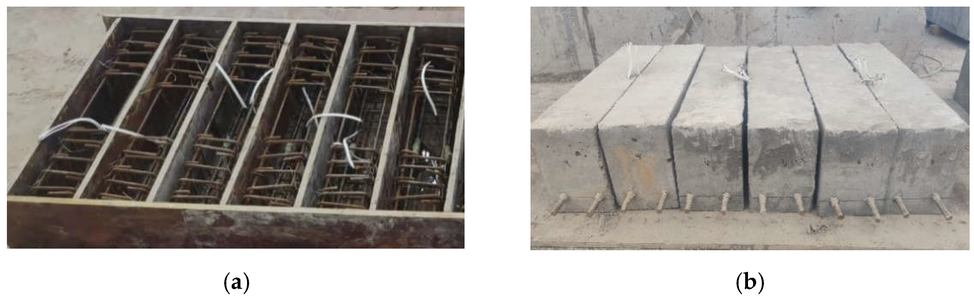
2.1. Specimens
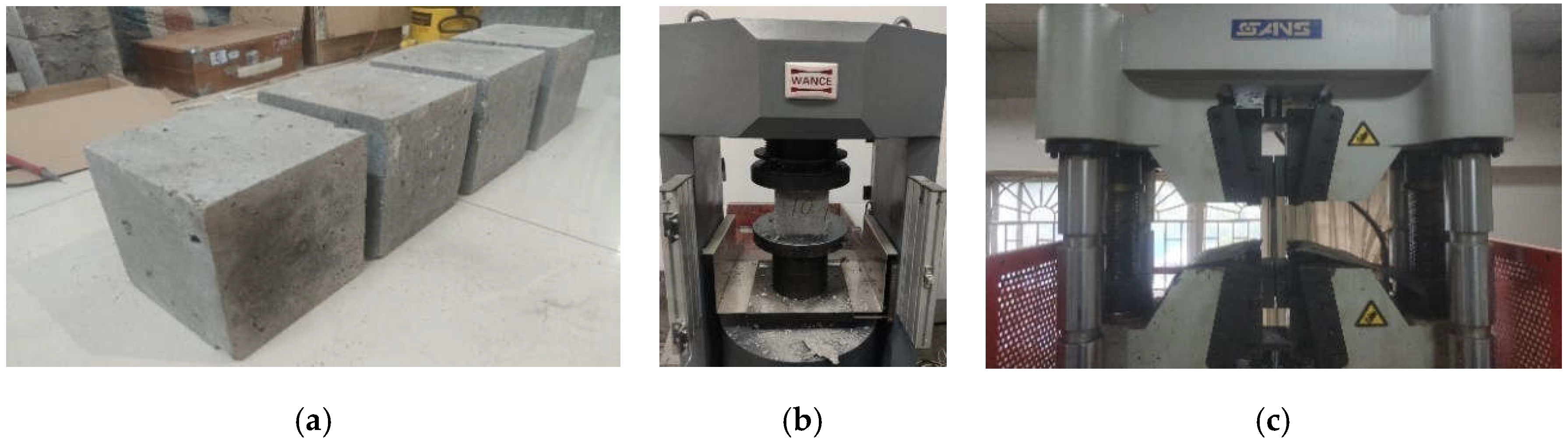
2.2. Material Properties
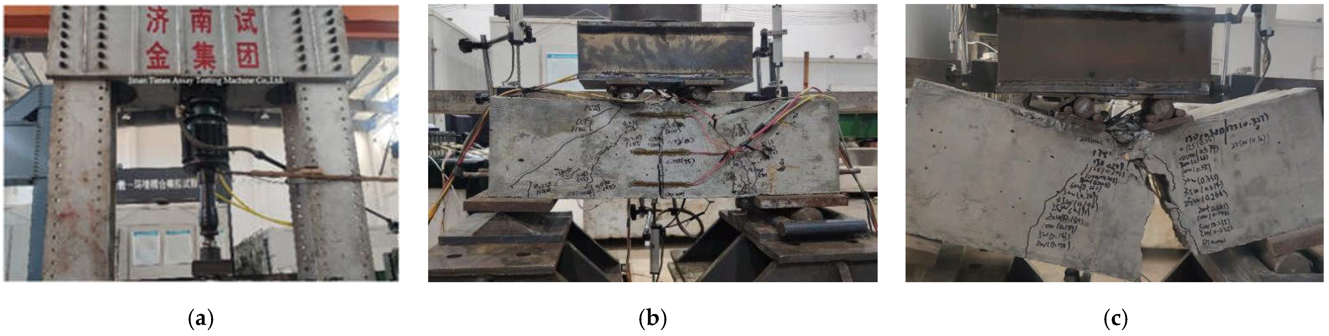
2.3. Test Loading Device and Loading System
2.4. Measurement Point Arrangement and Data Acquisition
2.5. Test Results and Analysis
3. Method
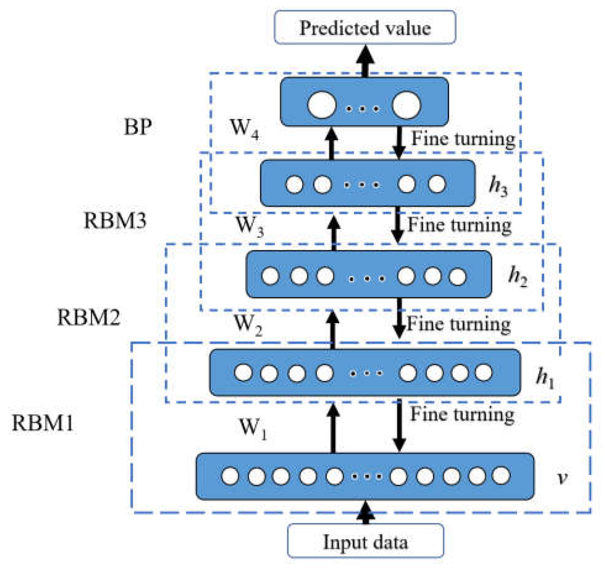
3.1. Principle of the DBN
3.2. Parameter Optimization based on the PSO Algorithm
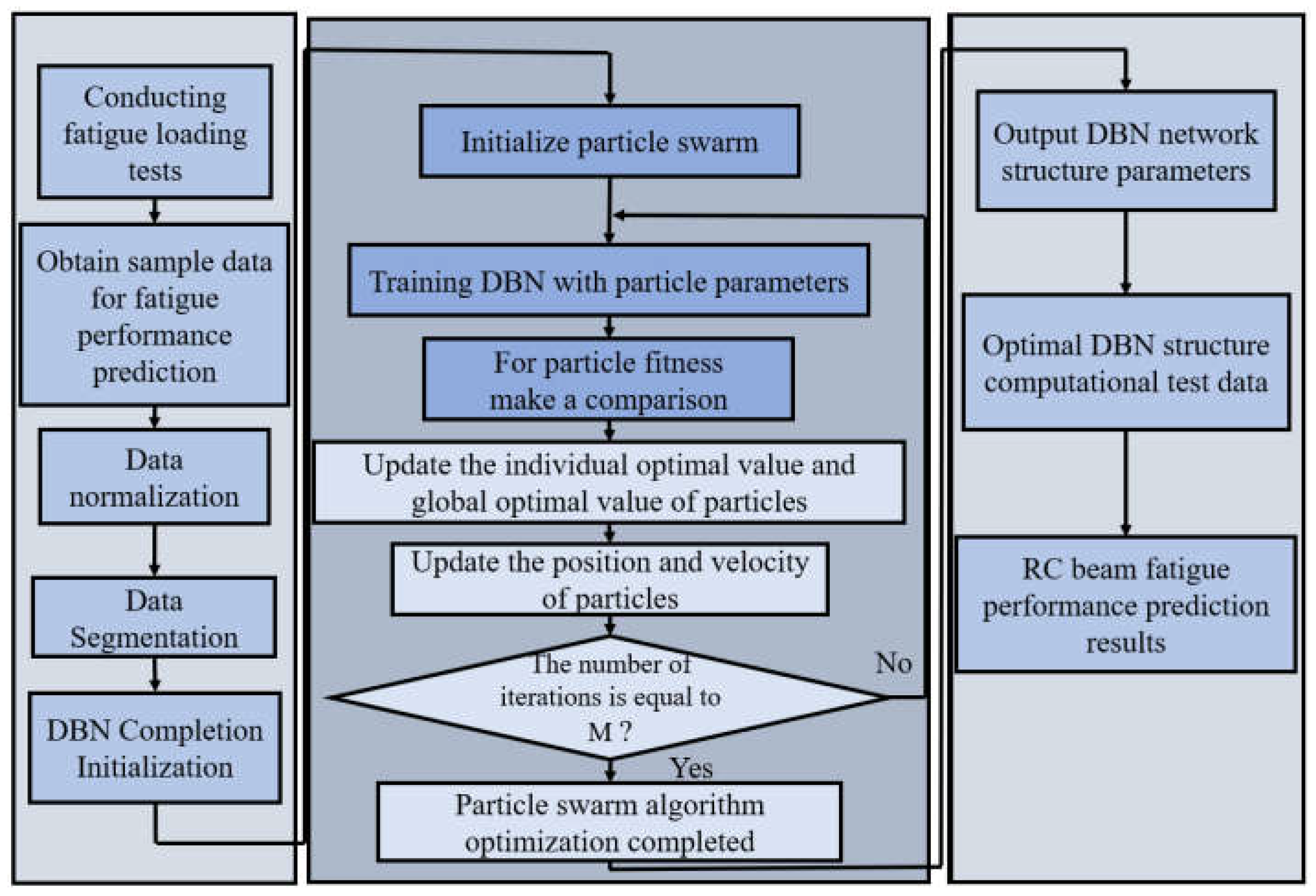
3.3. Fatigue Performance Prediction of RC Beams based on the PSO-DBN Model
3.4. Test Data Pre-Process
3.5. Evaluation Indicators
3.6. Model Parameter Setting
4. Results and Discussion
4.1. Prediction Capability of the PSO–DBN Model
4.2. Models Comparison and Analysis
5. Conclusion
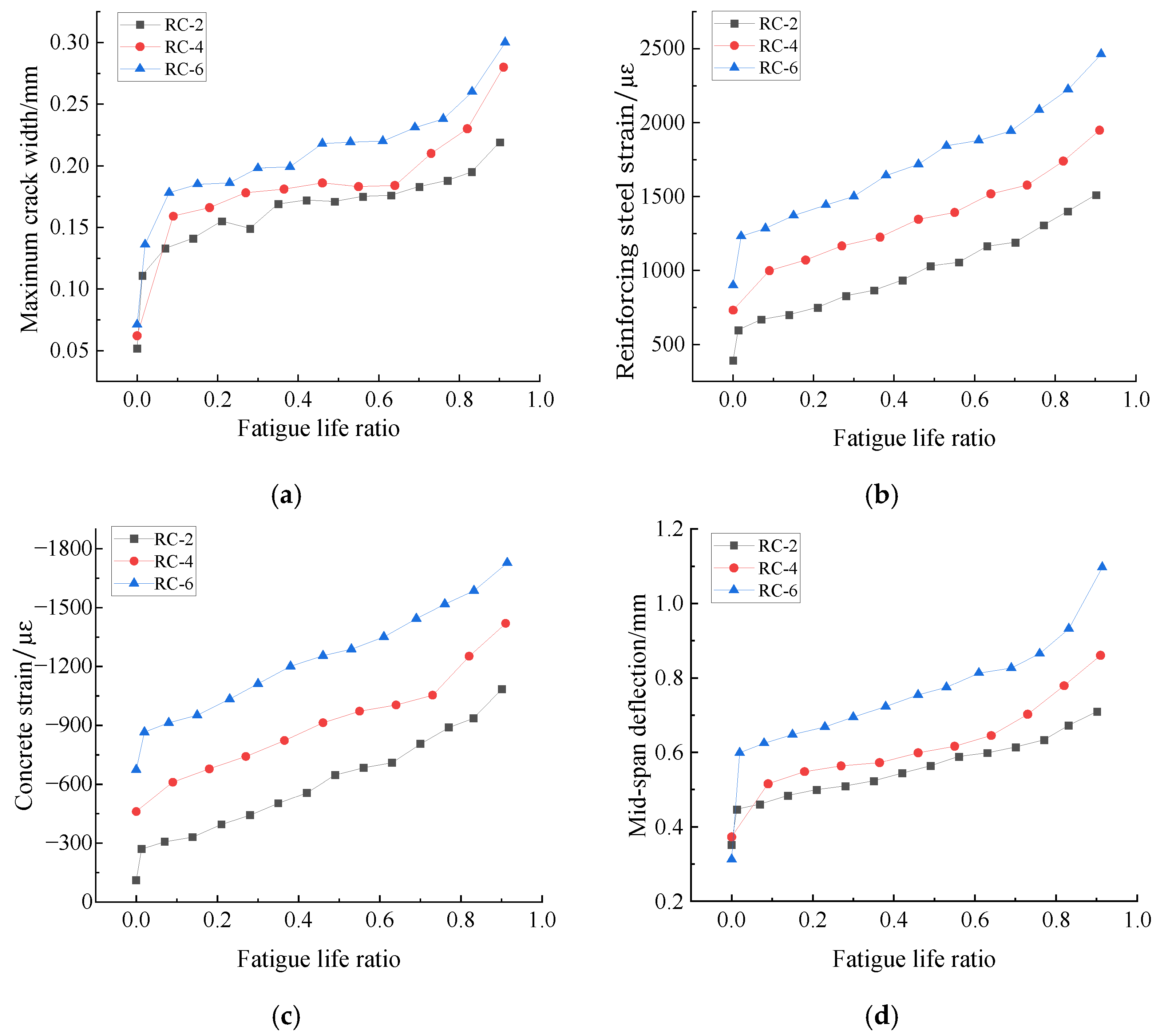
- Under the action of constantamplitude four-point bending cyclic loading, the mid-span deflection, tensile reinforcement strain, and concrete strain in the compression zone at the top of the beam of RC specimen beams with CRB600H for tensile reinforcement showed a three-stage trend at different damage stages with different static loading, i.e., rapid development at the initial stage, stable and slow development at the middle stage, and rapid development at the later stage until the fatigue fracture of the reinforcement.
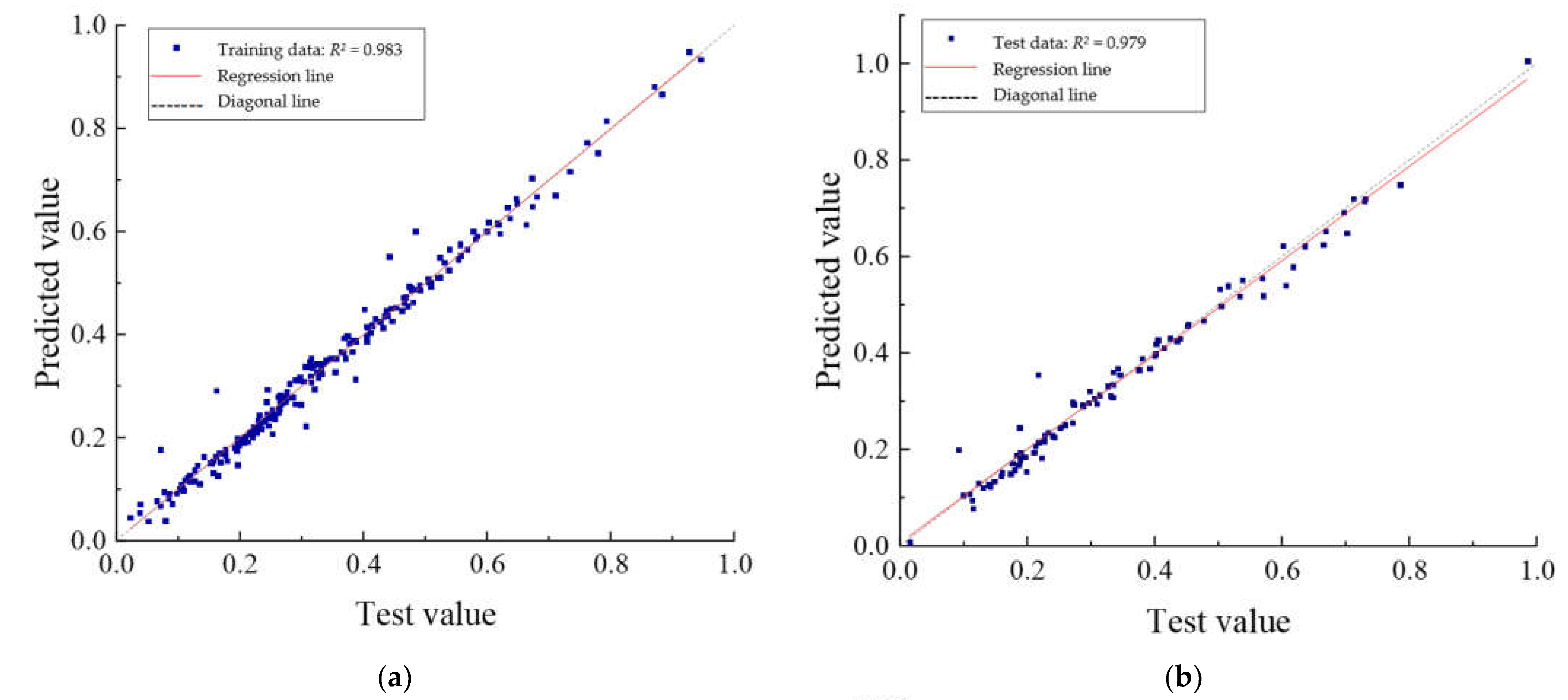
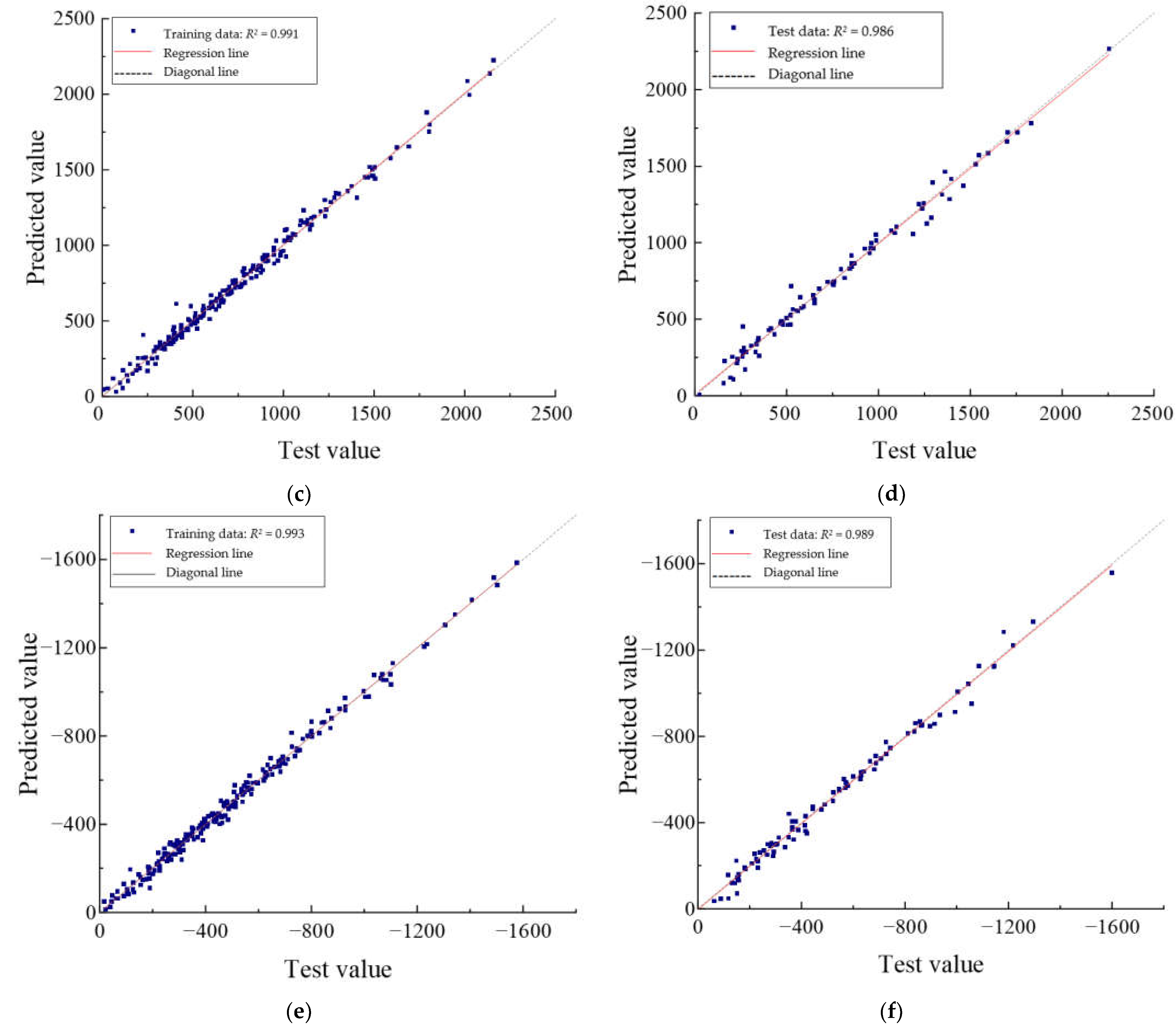
- The PSO-DBN model describes the complex nonlinear mapping relationship between the RC specimen beams and their material properties, load magnitude, and other factors and accurately predicts and reflects the real process of fatigue damage evolution of the RC specimen beams. By collecting the static loading time data of RC specimen beams at different damage stages during the fatigue loading test, a database containing 300 samples was established and used to train a DBN model. The parameters of the DBN model were adjusted by using PSO to establish the PSO-DBN model. Four evaluation metrics, namely root mean square error (RMSE), mean absolute error (MAE), mean absolute percentage error (MAPE), and coefficient of determination (R2), were used to evaluate the errors between the predicted values of the PSO-DBN model and test values. The prediction results of the PSO-DBN model showed high reliability, and in the three output vectors of the test section, the coefficient of determination (R2) reached 0.979, 0.986, and 0.989, respectively.
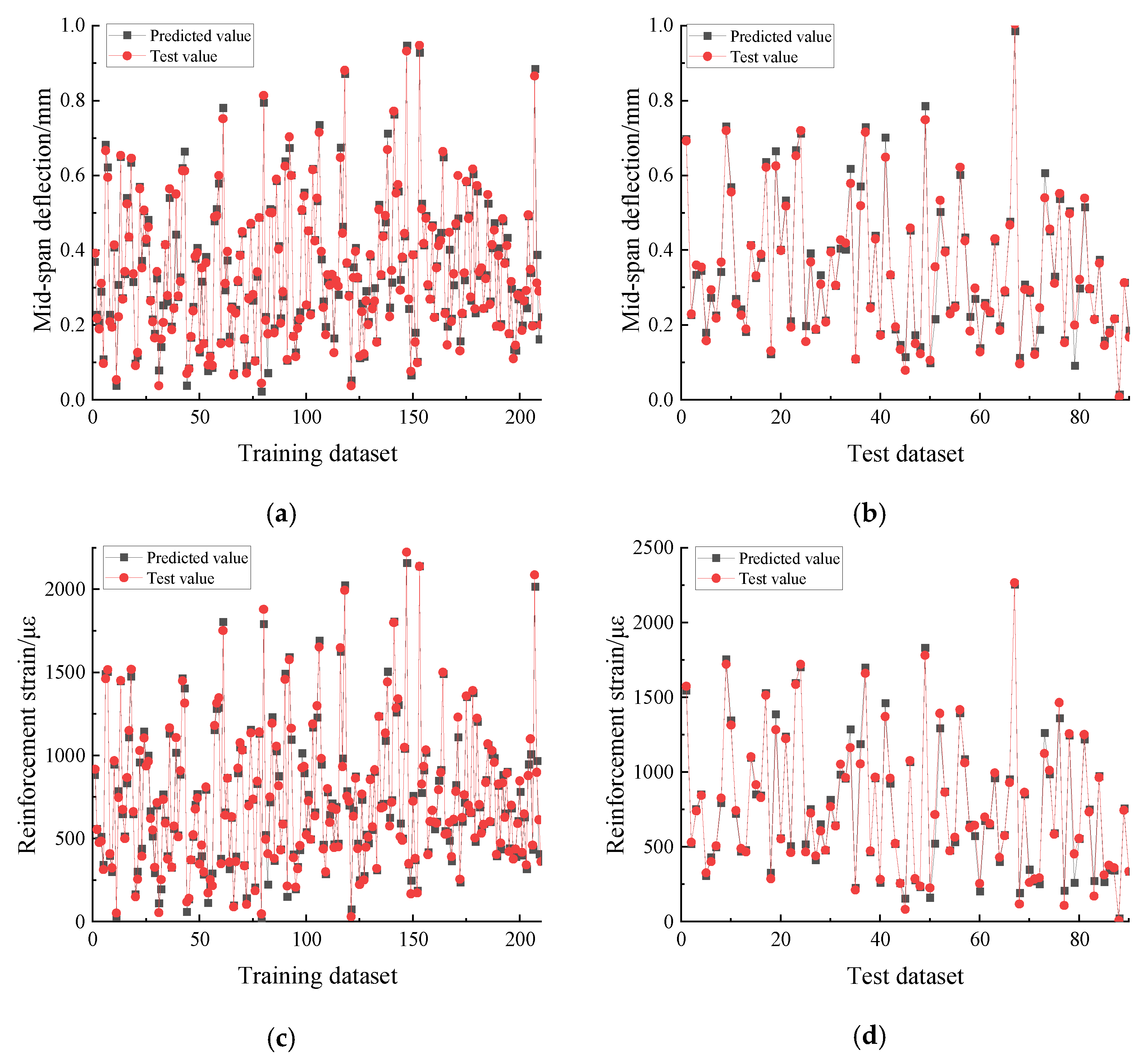
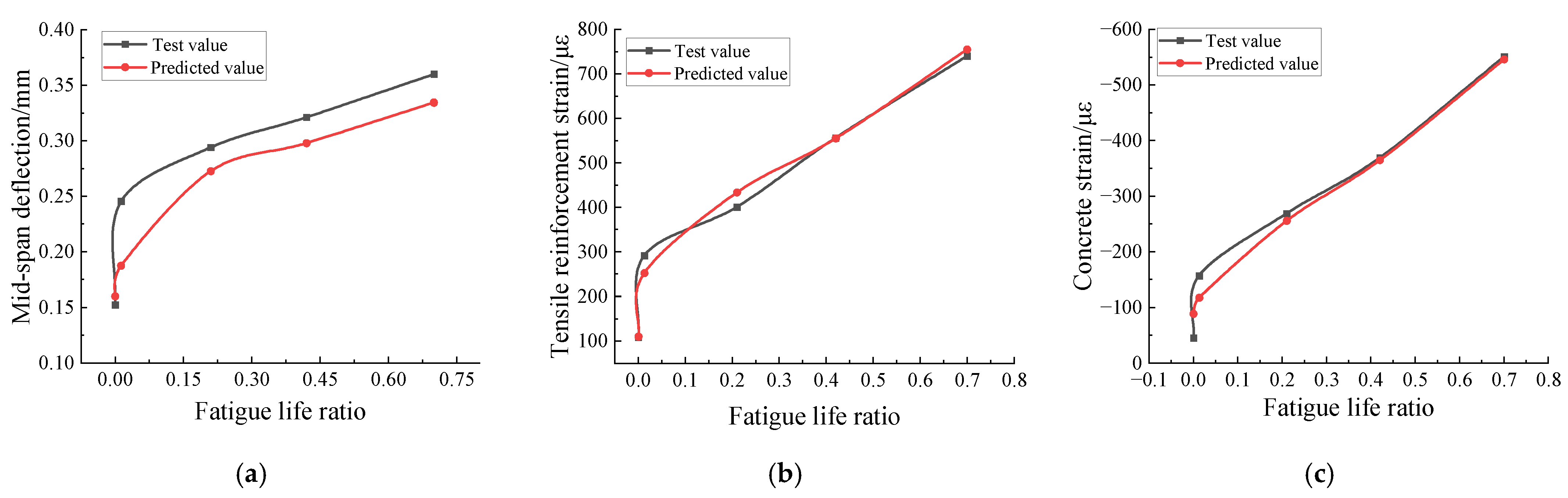
- The prediction performance of the model on the development process of mid-span deflection, reinforcement strain, and concrete strain in the compressive zone under cyclic loading of the specimen beams was analyzed by using an RC-2 specimen beam as an example. The results showed that the predicted values of mid-span deflection, strain in the tensile reinforcement, and concrete strain in the compression zone of the specimen beam under static load (25 kN) at different fatigue life ratios do not differ significantly from the tested values, and the model prediction of the development trend is consistent with the test results.
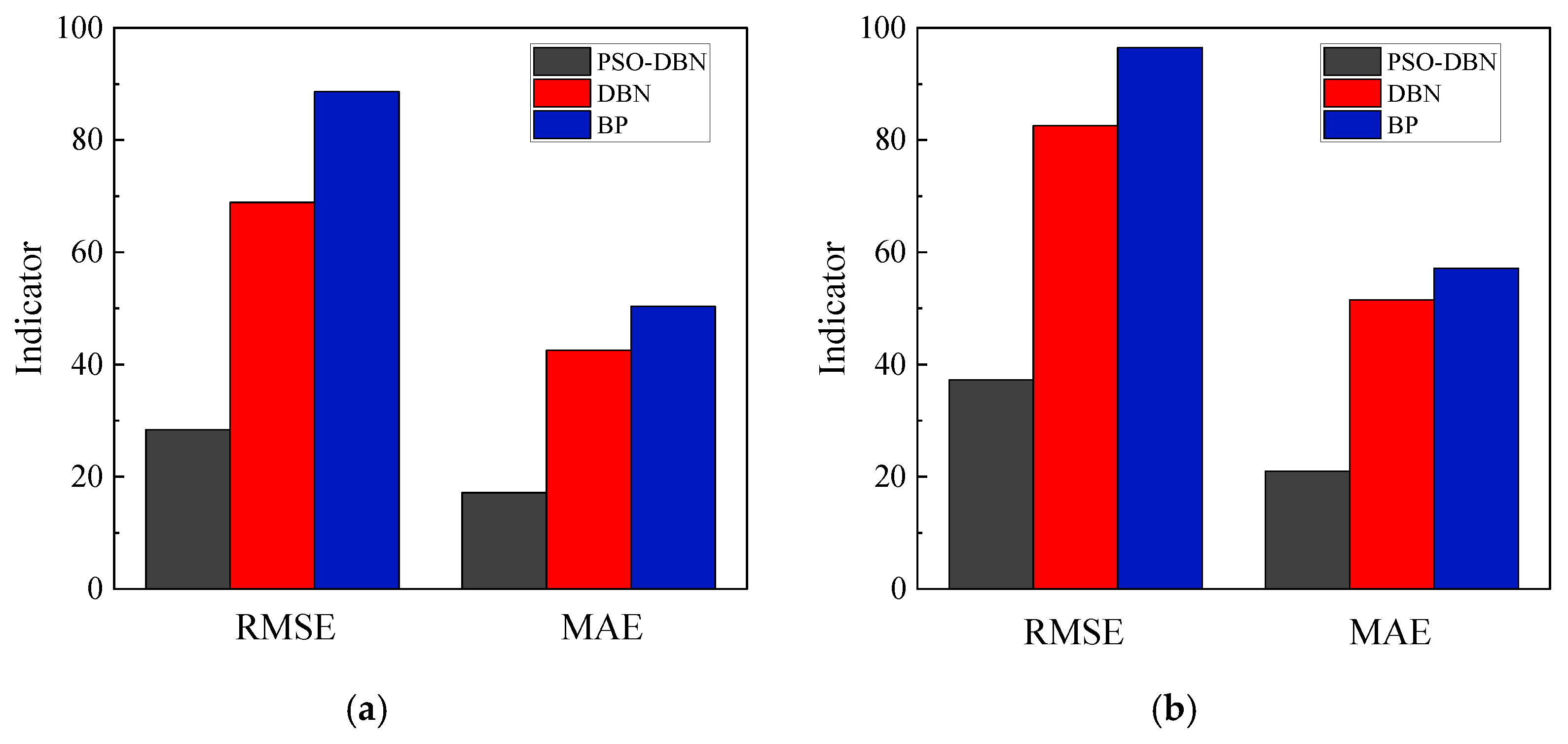
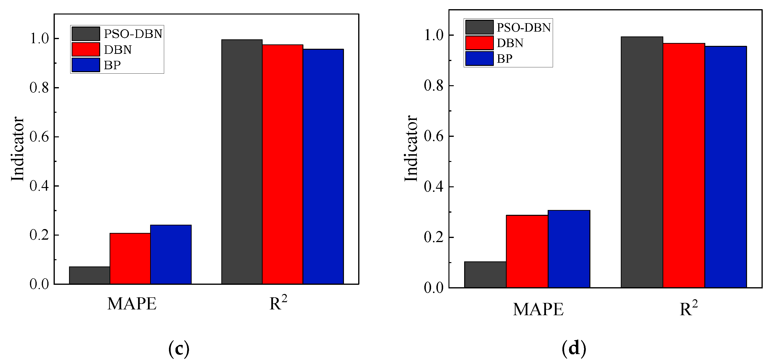
- The PSO-DBN model was compared with the single DBN model and BP model, and the comparison showed that the prediction performance of the PSO-DBN model is better, and the accuracy of RMSE, MAE, MAPE, and R2 are improved to different degrees. Focusing on the test set of the PSO-DBN model and the single DBN model, the average increases in RMSE, MAE, MAPE, and R2 reached 53.7%, 59.6%, 63.3%, and 6.0%, respectively. This indicated that the PSO-DBN model could predict the fatigue performance of RC specimen beams more efficiently and accurately.
Author Contributions
Funding
Institutional Review Board Statement
Informed Consent Statement
Data Availability Statement
Conflicts of Interest
Appendix A

| No. | Load Amplitude (kN) | Concrete Strength (MPa) | Static Loading Values (kN) | Fatigue Life Ratio(n/N) | Concrete Strain (με) | Tensile Reinforcement Strain (με) | Mid-Span Deflection (mm) |
|---|---|---|---|---|---|---|---|
| 1 | 60 | 55 | 35 | 0.73 | −660.207 | 917.4659 | 0.392024 |
| 2 | 80 | 63.7 | 15 | 0.3 | −348.898 | 555.1427 | 0.217485 |
| 3 | 60 | 55 | 10 | 0.55 | −325.581 | 475.9222 | 0.189237 |
| 4 | 30 | 36.9 | 25 | 0.35 | −355.138 | 483.8292 | 0.311466 |
| 5 | 80 | 63.7 | 50 | 0 | −208.525 | 313.328 | 0.096914 |
| 6 | 80 | 63.7 | 85 | 0.38 | −1080.04 | 1461.95 | 0.666317 |
| 7 | 60 | 55 | 55 | 0.91 | −1076.23 | 1516.539 | 0.594662 |
| 8 | 30 | 36.9 | 20 | 0.28 | −266.424 | 408.7969 | 0.208433 |
| 9 | 60 | 55 | 25 | 0.0914 | −262.274 | 323.9581 | 0.193996 |
| 10 | 60 | 55 | 45 | 0.64 | −691.86 | 968.367 | 0.414213 |
| 11 | 60 | 55 | 20 | 0 | −63.3075 | 52.00258 | 0.053224 |
| 12 | 60 | 55 | 25 | 0.46 | −447.674 | 522.91 | 0.253336 |
| 13 | 30 | 36.9 | 35 | 0.42 | −469.747 | 727.0375 | 0.451553 |
| 14 | 60 | 55 | 20 | 0.46 | −425.065 | 495.1695 | 0.22686 |
| 15 | 30 | 36.9 | 40 | 0.7 | −805.281 | 1190.168 | 0.61478 |
| 16 | 30 | 36.9 | 35 | 0.28 | −406.872 | 636.4812 | 0.424396 |
| 17 | 80 | 63.7 | 65 | 0.53 | −880.118 | 1298.979 | 0.539176 |
| 18 | 80 | 63.7 | 80 | 0.69 | −1216.69 | 1653.203 | 0.715272 |
| 19 | 80 | 63.7 | 40 | 0.61 | −622.718 | 982.8878 | 0.396408 |
| 20 | 60 | 55 | 35 | 0.1825 | −379.845 | 438.0652 | 0.246948 |
| 21 | 30 | 36.9 | 20 | 0.07 | −159.305 | 300.1294 | 0.173507 |
| 22 | 80 | 63.7 | 35 | 0.46 | −503.693 | 801.0338 | 0.334273 |
| 23 | 60 | 55 | 40 | 0.365 | −497.416 | 596.9282 | 0.306398 |
| 24 | 60 | 55 | 40 | 0.46 | −560.724 | 687.382 | 0.334973 |
| 25 | 80 | 63.7 | 60 | 0 | −330.364 | 447.4182 | 0.125569 |
| 26 | 80 | 63.7 | 40 | 0.23 | −401.207 | 675.1316 | 0.318897 |
| 27 | 30 | 36.9 | 25 | 0.28 | −313.223 | 450.194 | 0.303701 |
| 28 | 60 | 55 | 60 | 0.91 | −1130.49 | 1648.27 | 0.647523 |
| 29 | 60 | 55 | 60 | 0.365 | −664.729 | 933.771 | 0.445335 |
| 30 | 80 | 63.7 | 75 | 0.914 | −1416.27 | 1994.367 | 0.880539 |
| 31 | 60 | 55 | 45 | 0.46 | −587.855 | 755.7912 | 0.365869 |
| 32 | 80 | 63.7 | 80 | 0 | −564.464 | 747.5251 | 0.221702 |
| 33 | 30 | 36.9 | 20 | 0.77 | −520.255 | 724.4502 | 0.276353 |
| 34 | 30 | 36.9 | 10 | 0 | −14.4425 | 31.04787 | 0.037254 |
| 35 | 60 | 55 | 50 | 0.1825 | −438.63 | 634.1909 | 0.326397 |
| 36 | 80 | 63.7 | 55 | 0.23 | −587.363 | 863.5034 | 0.396788 |
| 37 | 30 | 36.9 | 30 | 0.139 | −243.594 | 439.8448 | 0.327171 |
| 38 | 30 | 36.9 | 0 | 0.42 | −146.709 | 222.5097 | 0.116433 |
| 39 | 80 | 63.7 | 10 | 0.61 | −421.279 | 768.7126 | 0.235399 |
| 40 | 30 | 36.9 | 0 | 0.49 | −176.977 | 250.9702 | 0.122254 |
| 41 | 60 | 55 | 40 | 0.1825 | −379.845 | 447.7179 | 0.264636 |
| 42 | 30 | 36.9 | 15 | 0.56 | −331.381 | 509.7025 | 0.20048 |
| 43 | 80 | 63.7 | 80 | 0.46 | −1060.82 | 1450.698 | 0.65326 |
| 44 | 60 | 55 | 45 | 0.55 | −669.251 | 855.2599 | 0.38785 |
| 45 | 30 | 36.9 | 20 | 0.56 | −406.139 | 571.7982 | 0.243361 |
| 46 | 80 | 63.7 | 0 | 0.83 | −577.03 | 913.6663 | 0.263571 |
| 47 | 30 | 36.9 | 10 | 0.35 | −172.779 | 320.8279 | 0.153683 |
| 48 | 60 | 55 | 55 | 0.73 | −836.563 | 1236.105 | 0.508962 |
| 49 | 80 | 63.7 | 45 | 0.15 | −406.738 | 684.7763 | 0.334508 |
| 50 | 30 | 36.9 | 35 | 0.35 | −444.129 | 690.815 | 0.436039 |
| 51 | 80 | 63.7 | 60 | 0.46 | −787.062 | 1134.657 | 0.492507 |
| 52 | 80 | 63.7 | 90 | 0.23 | −1033.62 | 1442.919 | 0.669016 |
| 53 | 60 | 55 | 10 | 0.73 | −420.543 | 575.3909 | 0.2222 |
| 54 | 30 | 36.9 | 20 | 0.7 | −482.986 | 675.2911 | 0.268582 |
| 55 | 60 | 55 | 30 | 0.64 | −587.855 | 717.8763 | 0.345753 |
| 56 | 80 | 63.7 | 65 | 0.914 | −1205.56 | 1799.656 | 0.771727 |
| 57 | 80 | 63.7 | 70 | 0.46 | −923.948 | 1286.304 | 0.552216 |
| 58 | 80 | 63.7 | 65 | 0.61 | −933.446 | 1342.031 | 0.575364 |
| 59 | 60 | 55 | 45 | 0.1825 | −416.021 | 511.5472 | 0.293324 |
| 60 | 30 | 36.9 | 35 | 0.07 | −250.819 | 489.0039 | 0.381702 |
| 61 | 60 | 55 | 45 | 0.73 | −737.08 | 1049.82 | 0.444983 |
| 62 | 80 | 63.7 | 90 | 0.83 | −1586.06 | 2224.26 | 0.932645 |
| 63 | 30 | 36.9 | 25 | 0.07 | −192.125 | 349.2885 | 0.268775 |
| 64 | 80 | 63.7 | 40 | 0 | −123.614 | 168.0645 | 0.075977 |
| 65 | 30 | 36.9 | 30 | 0.21 | −301.82 | 499.3532 | 0.342692 |
| 66 | 30 | 36.9 | 30 | 0.56 | −530.029 | 724.4502 | 0.38732 |
| 67 | 60 | 55 | 10 | 0.365 | −271.318 | 380.9899 | 0.154072 |
| 68 | 30 | 36.9 | 0 | 0.21 | −83.833 | 173.3506 | 0.098968 |
| 69 | 80 | 63.7 | 80 | 0.914 | −1484.71 | 2137.945 | 0.947851 |
| 70 | 30 | 36.9 | 40 | 0.28 | −441.995 | 827.9431 | 0.50999 |
| 71 | 80 | 63.7 | 55 | 0.3 | −629.749 | 935.2546 | 0.417464 |
| 72 | 60 | 55 | 65 | 0.2737 | −637.597 | 1033.863 | 0.484995 |
| 73 | 30 | 36.9 | 30 | 0.07 | −222.633 | 403.6223 | 0.307766 |
| 74 | 60 | 55 | 25 | 0.55 | −497.416 | 604.2764 | 0.268725 |
| 75 | 30 | 36.9 | 40 | 0.07 | −306.925 | 670.1164 | 0.461478 |
| 76 | 30 | 36.9 | 40 | 0.35 | −502.542 | 866.7529 | 0.523577 |
| 77 | 30 | 36.9 | 15 | 0.7 | −403.571 | 600.2587 | 0.219882 |
| 78 | 30 | 36.9 | 30 | 0.35 | −392.646 | 592.4968 | 0.352401 |
| 79 | 60 | 55 | 60 | 0.1825 | −560.724 | 793.6626 | 0.412368 |
| 80 | 60 | 55 | 60 | 0.2737 | −614.987 | 897.6098 | 0.425548 |
| 81 | 80 | 63.7 | 75 | 0.61 | −1053.91 | 1501.646 | 0.663472 |
| 82 | 80 | 63.7 | 20 | 0.23 | −328.464 | 526.5123 | 0.230504 |
| 83 | 80 | 63.7 | 65 | 0 | −382.39 | 530.4221 | 0.146402 |
| 84 | 30 | 36.9 | 40 | 0.013 | −269.66 | 597.6714 | 0.447885 |
| 85 | 60 | 55 | 25 | 0.1825 | −325.581 | 391.7876 | 0.209384 |
| 86 | 30 | 36.9 | 25 | 0.49 | −390.063 | 615.7827 | 0.33668 |
| 87 | 80 | 63.7 | 40 | 0.76 | −751.255 | 1150.314 | 0.43518 |
| 88 | 30 | 36.9 | 35 | 0.49 | −532.615 | 783.9586 | 0.470952 |
| 89 | 80 | 63.7 | 90 | 0.015 | −865.426 | 1230.836 | 0.599245 |
| 90 | 30 | 36.9 | 15 | 0.07 | −135.765 | 256.1449 | 0.130619 |
| 91 | 30 | 36.9 | 15 | 0.77 | −447.818 | 626.132 | 0.231531 |
| 92 | 60 | 55 | 35 | 0.55 | −574.289 | 763.7191 | 0.339269 |
| 93 | 60 | 55 | 65 | 0.64 | −917.959 | 1359.415 | 0.583906 |
| 94 | 30 | 36.9 | 40 | 0.139 | −330.215 | 701.1643 | 0.484757 |
| 95 | 80 | 63.7 | 25 | 0.38 | −435.185 | 658.9422 | 0.274556 |
| 96 | 60 | 55 | 70 | 0.55 | −972.222 | 1391.721 | 0.616983 |
| 97 | 60 | 55 | 60 | 0 | −307.494 | 504.2424 | 0.24312 |
| 98 | 60 | 55 | 70 | 0.64 | −1003.88 | 1518.409 | 0.645558 |
| 99 | 60 | 55 | 70 | 0.365 | −822.997 | 1224.365 | 0.57302 |
| 100 | 80 | 63.7 | 50 | 0.08 | −438.25 | 705.5755 | 0.34238 |
| 101 | 30 | 36.9 | 30 | 0.28 | −355.392 | 532.9884 | 0.352404 |
| 102 | 60 | 55 | 15 | 0.64 | −434.109 | 585.0146 | 0.24433 |
| 103 | 60 | 55 | 15 | 0.91 | −624.031 | 838.2156 | 0.323451 |
| 104 | 60 | 55 | 70 | 0.1825 | −678.295 | 1070.56 | 0.548837 |
| 105 | 30 | 36.9 | 20 | 0.63 | −448.065 | 602.8461 | 0.255001 |
| 106 | 80 | 63.7 | 45 | 0.61 | −663.809 | 1030.794 | 0.414616 |
| 107 | 80 | 63.7 | 65 | 0.15 | −673.632 | 959.3437 | 0.453897 |
| 108 | 60 | 55 | 55 | 0 | −239.664 | 404.194 | 0.196857 |
| 109 | 30 | 36.9 | 25 | 0.56 | −448.263 | 662.3545 | 0.336683 |
| 110 | 60 | 55 | 55 | 0.2737 | −560.724 | 829.1861 | 0.385882 |
| 111 | 30 | 36.9 | 15 | 0.49 | −287.127 | 473.4799 | 0.194658 |
| 112 | 30 | 36.9 | 35 | 0.56 | −588.502 | 835.705 | 0.484542 |
| 113 | 30 | 36.9 | 30 | 0.42 | −441.557 | 628.7193 | 0.364041 |
| 114 | 80 | 63.7 | 60 | 0.15 | −598.368 | 893.8788 | 0.412404 |
| 115 | 30 | 36.9 | 10 | 0.63 | −282.219 | 421.7335 | 0.176972 |
| 116 | 80 | 63.7 | 35 | 0.3 | −423.016 | 700.5784 | 0.316189 |
| 117 | 80 | 63.7 | 55 | 0 | −261.917 | 377.1777 | 0.109933 |
| 118 | 30 | 36.9 | 0 | 0.77 | −298.063 | 437.2574 | 0.145537 |
| 119 | 80 | 63.7 | 30 | 0.23 | −360.04 | 590.4656 | 0.279872 |
| 120 | 30 | 36.9 | 0 | 0.139 | −74.5224 | 150.0647 | 0.091206 |
| 121 | 80 | 63.7 | 20 | 0.61 | −504.851 | 847.0176 | 0.277024 |
| 122 | 60 | 55 | 15 | 0.365 | −339.147 | 417.7019 | 0.184982 |
| 123 | 60 | 55 | 20 | 0.64 | −483.85 | 648.9018 | 0.26422 |
| 124 | 30 | 36.9 | 30 | 0.013 | −171.396 | 341.5265 | 0.292246 |
| 125 | 30 | 36.9 | 35 | 0.63 | −625.755 | 879.6895 | 0.49425 |
| 126 | 80 | 63.7 | 0 | 0.914 | −620.784 | 1100.229 | 0.348846 |
| 127 | 80 | 63.7 | 20 | 0.08 | −260.09 | 461.1366 | 0.19692 |
| 128 | 80 | 63.7 | 90 | 0.76 | −1517.7 | 2087.133 | 0.865453 |
| 129 | 80 | 63.7 | 90 | 0 | −673.995 | 899.1677 | 0.312398 |
| 130 | 80 | 63.7 | 45 | 0.015 | −308.294 | 613.0197 | 0.29058 |
| 131 | 30 | 36.9 | 0 | 0.56 | -190.948 | 256.1449 | 0.126135 |
| 132 | 30 | 36.9 | 20 | 0.21 | −217.519 | 362.2251 | 0.200671 |
| 133 | 80 | 63.7 | 85 | 0.46 | −1125.17 | 1573.565 | 0.692161 |
| 134 | 60 | 55 | 15 | 0.55 | −388.889 | 530.751 | 0.228942 |
| 135 | 30 | 36.9 | 25 | 0.7 | −550.725 | 739.9741 | 0.359972 |
| 136 | 60 | 55 | 25 | 0.82 | −637.597 | 843.9405 | 0.354446 |
| 137 | 30 | 36.9 | 15 | 0.21 | −184.665 | 326.0026 | 0.157789 |
| 138 | 30 | 36.9 | 25 | 0.21 | −268.976 | 401.0349 | 0.293999 |
| 139 | 80 | 63.7 | 20 | 0.15 | −297.01 | 507.3762 | 0.217584 |
| 140 | 60 | 55 | 35 | 0.64 | −614.987 | 827.0266 | 0.367848 |
| 141 | 60 | 55 | 65 | 0.91 | −1284.24 | 1721.1 | 0.720159 |
| 142 | 30 | 36.9 | 40 | 0.49 | −646.926 | 1029.754 | 0.564327 |
| 143 | 60 | 55 | 60 | 0.73 | −899.871 | 1313.573 | 0.555243 |
| 144 | 80 | 63.7 | 20 | 0.53 | −463.83 | 743.3757 | 0.256352 |
| 145 | 30 | 36.9 | 20 | 0.42 | −329.307 | 489.0039 | 0.2259 |
| 146 | 30 | 36.9 | 10 | 0.7 | −333.441 | 465.718 | 0.188612 |
| 147 | 80 | 63.7 | 30 | 0.83 | −710.091 | 1102.311 | 0.41166 |
| 148 | 80 | 63.7 | 30 | 0.61 | −556.948 | 915.7463 | 0.331556 |
| 149 | 80 | 63.7 | 50 | 0.3 | −579.093 | 829.9471 | 0.388912 |
| 150 | 80 | 63.7 | 60 | 0.83 | −1044.13 | 1514.141 | 0.621715 |
| 151 | 30 | 36.9 | 0 | 0.63 | −221.22 | 287.1928 | 0.130013 |
| 152 | 80 | 63.7 | 90 | 0.08 | −913.284 | 1283.451 | 0.625089 |
| 153 | 30 | 36.9 | 40 | 0 | −111.316 | 393.273 | 0.352791 |
| 154 | 30 | 36.9 | 35 | 0.139 | −299.727 | 553.6869 | 0.399166 |
| 155 | 60 | 55 | 60 | 0.64 | −850.129 | 1223.162 | 0.517877 |
| 156 | 80 | 63.7 | 10 | 0.23 | −264.031 | 462.5689 | 0.194059 |
| 157 | 60 | 55 | 65 | 0.82 | −1125.97 | 1585.47 | 0.652035 |
| 158 | 80 | 63.7 | 60 | 0.914 | −1123.44 | 1719.841 | 0.719911 |
| 159 | 80 | 63.7 | 0 | 0.3 | −243.391 | 465.6075 | 0.155043 |
| 160 | 60 | 55 | 55 | 0.1825 | −501.938 | 725.2099 | 0.368299 |
| 161 | 80 | 63.7 | 15 | 0.08 | −260.019 | 440.3374 | 0.189057 |
| 162 | 60 | 55 | 45 | 0.2737 | −461.24 | 606.4939 | 0.308701 |
| 163 | 80 | 63.7 | 15 | 0.15 | −291.468 | 478.6043 | 0.207145 |
| 164 | 60 | 55 | 60 | 0.55 | −818.475 | 1105.62 | 0.506877 |
| 165 | 30 | 36.9 | 30 | 0.63 | −585.923 | 768.4347 | 0.395082 |
| 166 | 80 | 63.7 | 40 | 0.15 | −351.977 | 640.0501 | 0.305977 |
| 167 | 60 | 55 | 35 | 0.82 | −773.256 | 1053.11 | 0.427178 |
| 168 | 60 | 55 | 40 | 0.73 | −696.382 | 963.2508 | 0.4185 |
| 169 | 80 | 63.7 | 85 | 0.08 | −858.519 | 1163.771 | 0.578445 |
| 170 | 30 | 36.9 | 0 | 0.35 | −118.762 | 212.1604 | 0.108668 |
| 171 | 80 | 63.7 | 80 | 0.08 | −822.899 | 1055.271 | 0.518868 |
| 172 | 80 | 63.7 | 75 | 0.76 | −1220.73 | 1661.099 | 0.715156 |
| 173 | 60 | 55 | 30 | 0.2737 | −406.977 | 473.6757 | 0.244651 |
| 174 | 60 | 55 | 55 | 0.46 | −646.641 | 964.874 | 0.429834 |
| 175 | 60 | 55 | 50 | 0.55 | −691.86 | 937.2205 | 0.429704 |
| 176 | 60 | 55 | 20 | 0.0914 | −253.23 | 282.6227 | 0.171915 |
| 177 | 80 | 63.7 | 90 | 0.15 | −951.575 | 1371.154 | 0.648344 |
| 178 | 80 | 63.7 | 20 | 0.76 | −601.937 | 960.232 | 0.333863 |
| 179 | 30 | 36.9 | 10 | 0.77 | −366.052 | 522.6391 | 0.194437 |
| 180 | 30 | 36.9 | 10 | 0.21 | −137.858 | 256.1449 | 0.134281 |
| 181 | 30 | 36.9 | 20 | 0 | −35.8745 | 82.79431 | 0.07841 |
| 182 | 80 | 63.7 | 55 | 0.53 | −745.969 | 1077.171 | 0.458812 |
| 183 | 30 | 36.9 | 15 | 0.139 | −159.051 | 287.1928 | 0.150027 |
| 184 | 30 | 36.9 | 10 | 0.139 | −119.225 | 238.0336 | 0.122632 |
| 185 | 80 | 63.7 | 75 | 0.83 | −1331.49 | 1780.697 | 0.748748 |
| 186 | 80 | 63.7 | 70 | 0.08 | −705.165 | 964.2066 | 0.461785 |
| 187 | 60 | 55 | 0 | 0.0914 | −144.703 | 226.0837 | 0.105498 |
| 188 | 80 | 63.7 | 55 | 0.015 | −441.049 | 716.811 | 0.355436 |
| 189 | 80 | 63.7 | 35 | 0.914 | −812.722 | 1392.608 | 0.533239 |
| 190 | 60 | 55 | 50 | 0.46 | −601.421 | 864.8691 | 0.394546 |
| 191 | 60 | 55 | 25 | 0.365 | −406.977 | 473.1684 | 0.229157 |
| 192 | 80 | 63.7 | 35 | 0.08 | −284.91 | 565.0405 | 0.246409 |
| 193 | 80 | 63.7 | 70 | 0.61 | −1005.99 | 1417.061 | 0.621988 |
| 194 | 80 | 63.7 | 45 | 0.69 | −718.497 | 1062.686 | 0.424956 |
| 195 | 80 | 63.7 | 0 | 0.53 | −319.963 | 628.2452 | 0.183467 |
| 196 | 60 | 55 | 65 | 0 | −379.845 | 644.9741 | 0.298164 |
| 197 | 60 | 55 | 15 | 0.73 | −479.328 | 621.1758 | 0.26411 |
| 198 | 60 | 55 | 10 | 0.0914 | −189.922 | 254.375 | 0.127698 |
| 199 | 80 | 63.7 | 20 | 0.46 | −431.013 | 698.7271 | 0.251184 |
| 200 | 60 | 55 | 0 | 0.82 | −483.85 | 655.6703 | 0.235172 |
| 201 | 80 | 63.7 | 55 | 0.38 | −684.439 | 995.8504 | 0.43038 |
| 202 | 30 | 36.9 | 15 | 0.42 | −249.858 | 429.4955 | 0.184953 |
| 203 | 60 | 55 | 35 | 0.365 | −474.806 | 573.7242 | 0.290911 |
| 204 | 60 | 55 | 65 | 0.1825 | −619.509 | 929.8723 | 0.467416 |
| 205 | 80 | 63.7 | 85 | 0.914 | −1558.62 | 2267.204 | 1.004806 |
| 206 | 60 | 55 | 40 | 0 | −131.137 | 117.5566 | 0.095419 |
| 207 | 80 | 63.7 | 20 | 0.69 | −541.768 | 864.5592 | 0.295112 |
| 208 | 30 | 36.9 | 15 | 0.63 | −340.703 | 551.0996 | 0.208239 |
| 209 | 30 | 36.9 | 35 | 0 | −71.5098 | 261.3195 | 0.292439 |
| 210 | 60 | 55 | 0 | 0.2737 | −189.922 | 284.8837 | 0.120883 |
| 211 | 30 | 36.9 | 25 | 0.013 | −157.2 | 292.3674 | 0.245483 |
| 212 | 80 | 63.7 | 80 | 0.15 | −847.513 | 1123.831 | 0.539548 |
| 213 | 80 | 63.7 | 60 | 0.3 | −674.937 | 1011.873 | 0.456336 |
| 214 | 60 | 55 | 50 | 0.0914 | −361.757 | 584.4493 | 0.311015 |
| 215 | 80 | 63.7 | 40 | 0.914 | −853.809 | 1464.446 | 0.551451 |
| 216 | 30 | 36.9 | 25 | 0 | −45.4206 | 108.6675 | 0.152333 |
| 217 | 80 | 63.7 | 50 | 0.76 | −860.768 | 1257.274 | 0.497423 |
| 218 | 80 | 63.7 | 25 | 0.015 | −221.873 | 453.2468 | 0.199628 |
| 219 | 60 | 55 | 15 | 0.1825 | −289.406 | 327.2771 | 0.165199 |
| 220 | 30 | 36.9 | 25 | 0.42 | −369.113 | 556.2743 | 0.321162 |
| 221 | 80 | 63.7 | 60 | 0.61 | −869.106 | 1251.055 | 0.539027 |
| 222 | 60 | 55 | 15 | 0.82 | −560.724 | 734.2249 | 0.297077 |
| 223 | 30 | 36.9 | 30 | 0 | −47.9772 | 170.7633 | 0.214616 |
| 224 | 80 | 63.7 | 35 | 0.69 | −633.598 | 963.6751 | 0.365276 |
| 225 | 60 | 55 | 10 | 0.1825 | −230.62 | 313.175 | 0.145281 |
| 226 | 60 | 55 | 15 | 0.2737 | −302.972 | 376.9897 | 0.178389 |
| 227 | 60 | 55 | 30 | 0.0914 | −298.45 | 360.6411 | 0.216083 |
| 228 | 30 | 36.9 | 0 | 0 | −11.6504 | 7.761966 | 0.007774 |
| 229 | 60 | 55 | 25 | 0.73 | −569.767 | 744.4718 | 0.312684 |
| 230 | 30 | 36.9 | 25 | 0.63 | −483.184 | 716.6882 | 0.342501 |
| 231 | 30 | 36.9 | 15 | 0.28 | −210.283 | 336.3519 | 0.167488 |
| 232 | 30 | 36.9 | 15 | 0 | −23.9923 | 54.33376 | 0.037457 |
| 233 | 30 | 36.9 | 20 | 0.013 | −129.026 | 253.5576 | 0.161864 |
| 234 | 80 | 63.7 | 0 | 0.69 | −410.211 | 735.0806 | 0.206719 |
| 235 | 30 | 36.9 | 35 | 0.21 | −346.317 | 592.4968 | 0.414693 |
| 236 | 30 | 36.9 | 25 | 0.139 | −229.379 | 377.749 | 0.278475 |
| 237 | 60 | 55 | 70 | 0.2737 | −741.602 | 1165.551 | 0.564225 |
| 238 | 60 | 55 | 20 | 0.1825 | −316.537 | 327.8714 | 0.187304 |
| 239 | 60 | 55 | 20 | 0.55 | −438.63 | 576.5359 | 0.244439 |
| 240 | 80 | 63.7 | 85 | 0.015 | −814.764 | 1107.967 | 0.550017 |
| 241 | 60 | 55 | 35 | 0.2737 | −420.543 | 510.4022 | 0.27772 |
| 242 | 80 | 63.7 | 25 | 0.69 | −591.067 | 909.2862 | 0.315891 |
| 243 | 60 | 55 | 65 | 0.73 | −976.744 | 1449.898 | 0.612478 |
| 244 | 80 | 63.7 | 85 | 0.23 | −978.863 | 1315.242 | 0.612036 |
| 245 | 30 | 36.9 | 0 | 0.013 | −48.9041 | 119.0168 | 0.069858 |
| 246 | 30 | 36.9 | 0 | 0.07 | −62.8757 | 139.7154 | 0.081504 |
| 247 | 30 | 36.9 | 10 | 0.49 | −230.99 | 372.5744 | 0.169207 |
| 248 | 30 | 36.9 | 20 | 0.49 | −359.571 | 522.6391 | 0.23754 |
| 249 | 30 | 36.9 | 30 | 0.49 | −485.801 | 677.8784 | 0.383442 |
| 250 | 60 | 55 | 60 | 0.0914 | −497.416 | 743.921 | 0.392581 |
| 251 | 30 | 36.9 | 0 | 0.7 | −263.138 | 346.7012 | 0.135834 |
| 252 | 30 | 36.9 | 35 | 0.013 | −206.59 | 460.5433 | 0.352595 |
| 253 | 30 | 36.9 | 10 | 0.28 | −149.493 | 300.1294 | 0.149805 |
| 254 | 60 | 55 | 50 | 0.365 | −538.114 | 810.6055 | 0.365968 |
| 255 | 30 | 36.9 | 10 | 0.013 | −77.3182 | 173.3506 | 0.093525 |
| 256 | 60 | 55 | 0 | 0.1825 | −176.357 | 253.2155 | 0.114289 |
| 257 | 80 | 63.7 | 45 | 0 | −153.762 | 215.9824 | 0.091605 |
| 258 | 60 | 55 | 45 | 0.82 | −813.953 | 1180.914 | 0.488939 |
| 259 | 80 | 63.7 | 45 | 0.83 | −860.708 | 1314.618 | 0.49214 |
| 260 | 60 | 55 | 70 | 0.46 | −913.437 | 1346.487 | 0.5994 |
| 261 | 60 | 55 | 0 | 0.46 | −239.664 | 348.1767 | 0.149454 |
| 262 | 80 | 63.7 | 80 | 0.76 | −1302.84 | 1752.072 | 0.75146 |
| 263 | 60 | 55 | 30 | 0.55 | −547.158 | 641.0174 | 0.310592 |
| 264 | 60 | 55 | 40 | 0.64 | −651.163 | 863.7965 | 0.396525 |
| 265 | 60 | 55 | 10 | 0.2737 | −257.752 | 358.3801 | 0.151878 |
| 266 | 80 | 63.7 | 20 | 0.38 | −398.196 | 631.7532 | 0.243432 |
| 267 | 60 | 55 | 30 | 0 | −90.4393 | 89.29429 | 0.066604 |
| 268 | 60 | 55 | 35 | 0.0914 | −307.494 | 361.2064 | 0.231552 |
| 269 | 80 | 63.7 | 15 | 0.76 | −545.795 | 923.4785 | 0.318252 |
| 270 | 80 | 63.7 | 25 | 0.83 | −699.089 | 1076.716 | 0.385663 |
| 271 | 60 | 55 | 50 | 0.64 | −732.558 | 1032.153 | 0.449484 |
| 272 | 30 | 36.9 | 10 | 0.42 | −189.083 | 336.3519 | 0.163386 |
| 273 | 60 | 55 | 35 | 0 | −90.4393 | 103.4109 | 0.071123 |
| 274 | 60 | 55 | 10 | 0.82 | −501.938 | 697.4839 | 0.270548 |
| 275 | 80 | 63.7 | 50 | 0.69 | −800.603 | 1136.097 | 0.471592 |
| 276 | 60 | 55 | 0 | 0.91 | −547.158 | 737.0656 | 0.281322 |
| 277 | 30 | 36.9 | 0 | 0.28 | −104.79 | 186.2872 | 0.102846 |
| 278 | 80 | 63.7 | 35 | 0.53 | −535.146 | 845.6807 | 0.342024 |
| 279 | 60 | 55 | 55 | 0.64 | −795.866 | 1141.158 | 0.486981 |
| 280 | 60 | 55 | 15 | 0 | −49.7416 | 46.91537 | 0.044319 |
| 281 | 80 | 63.7 | 90 | 0.61 | −1350.86 | 1879.832 | 0.813765 |
| 282 | 80 | 63.7 | 15 | 0.23 | −318.818 | 496.146 | 0.212317 |
| 283 | 80 | 63.7 | 15 | 0.015 | −194.387 | 408.445 | 0.176141 |
| 284 | 30 | 36.9 | 40 | 0.21 | −395.415 | 750.3234 | 0.500284 |
| 285 | 80 | 63.7 | 55 | 0.69 | −863.565 | 1193.574 | 0.50016 |
| 286 | 30 | 36.9 | 15 | 0.35 | −242.891 | 380.3364 | 0.179131 |
| 287 | 30 | 36.9 | 40 | 0.56 | −684.183 | 1055.627 | 0.589556 |
| 288 | 30 | 36.9 | 30 | 0.7 | −637.152 | 817.5938 | 0.402844 |
| 289 | 60 | 55 | 20 | 0.365 | −384.367 | 431.8475 | 0.204882 |
| 290 | 60 | 55 | 30 | 0.46 | −506.46 | 586.7393 | 0.288611 |
| 291 | 80 | 63.7 | 70 | 0.69 | −1079.83 | 1458.513 | 0.624568 |
| 292 | 30 | 36.9 | 15 | 0.013 | −96.1786 | 214.7477 | 0.107333 |
| 293 | 60 | 55 | 70 | 0.73 | −1053.62 | 1577.165 | 0.702711 |
| 294 | 30 | 36.9 | 40 | 0.63 | −709.805 | 1164.295 | 0.599259 |
| 295 | 30 | 36.9 | 10 | 0.56 | −263.59 | 385.511 | 0.169207 |
| 296 | 30 | 36.9 | 10 | 0.07 | −105.254 | 206.9858 | 0.11487 |
| 297 | 30 | 36.9 | 20 | 0.139 | −198.898 | 318.2406 | 0.190971 |
| 298 | 30 | 36.9 | 20 | 0.35 | −306.021 | 457.956 | 0.216198 |
| 299 | 30 | 36.9 | 35 | 0.7 | −695.62 | 926.2613 | 0.507831 |
| 300 | 30 | 36.9 | 40 | 0.42 | −556.114 | 934.0233 | 0.544925 |
References
- Niu, D.; Miao, Y. Experimental study on fatigue performance of corroded highway bridges based on vehicle loading. China Civ. Eng. J. 2018, 51, 112308. [Google Scholar]
- Nor, N.M.; Saliah, S.N.M.; Hashim, K.A. Fatigue damage assessment of reinforced concrete beam using average frequency and rise angle value of acoustic emission signal. Int. J. Struct. Integr. 2020, 11, 633–643. [Google Scholar] [CrossRef]
- Liu, F.; Zhou, J.; Yan, L. Study of stiffness and bearing capacity degradation of reinforced concrete beams under constant-amplitude fatigue. PLoS ONE 2018, 13, e0192797. [Google Scholar] [CrossRef] [PubMed]
- Liang, J.; Ding, Z.; Li, J. Analytical method for fatigue process of concrete structures. J. Build. Struct. 2017, 38, 149–157. [Google Scholar]
- Huang, B.-T.; Li, Q.-H.; Xu, S.-L.; Zhang, L. Static and fatigue performance of reinforced concrete beam strengthened with strain-hardening fiber-reinforced cementitious composite. Eng. Struct. 2019, 199, 109576. [Google Scholar] [CrossRef]
- Chen, Z.; Huang, P. Experimental Study on Fatigue Performance of CFRP-RC Beams Under Variable Amplitude Overloads. In Proceedings of the International Conference on Theoretical, Applied and Experimental Mechanics, Cyprus, Greece, 17–20 June 2018; pp. 152–154. [Google Scholar]
- Zhao, Y.; Wang, Z.; Xie, Y.; Wang, L. Experimental study on flexural behavior and fatigue life of steel fiber reinforced concrete beams. Concrete 2018, 5, 42–50. [Google Scholar]
- Wang, Y.; Li, J. Experimental study on stochastic responses of reinforced concrete beams under fatigue loading. Int. J. Fatigue 2021, 151, 106347. [Google Scholar] [CrossRef]
- Yang, J.; Zhang, T.; Sun, Q. Experimental study on flexural fatigue properties of reinforced concrete beams after salt freezing. Adv. Mater. Sci. Eng. 2020, 2020, 1032317. [Google Scholar] [CrossRef]
- Wang, X.; Zhou, C.; Ai, J.; Petrů, M.; Liu, Y. Numerical investigation for the fatigue performance of reinforced concrete beams strengthened with external prestressed HFRP sheet. Constr. Build. Mater. 2020, 237, 117601. [Google Scholar] [CrossRef]
- Banjara, N.K.; Ramanjaneyulu, K.; Sasmal, S.; Srinivas, V. Flexural fatigue performance of plain and fibre reinforced concrete. Trans. Indian Inst. Met. 2016, 69, 373–377. [Google Scholar] [CrossRef]
- Zhao, G.Q.; Li, K.; Zhang, L. Finite Element Analysis of Fatigue Performance for HRBF500 Reinforced Concrete Beams. J. Zhengzhou Univ. Eng. Sci. 2010, 31, 10–13. [Google Scholar]
- Jin, L.; Lan, Y.; Zhang, R.; Du, X. Numerical analysis of the mechanical behavior of the impact-damaged RC beams strengthened with CFRP. Compos. Struct. 2021, 274, 114353. [Google Scholar] [CrossRef]
- Qingfeng, H.; Jiang, L.; Leiyang, Y.; Jiawei, M. Numerical Simulation on Impact Test of CFRP Strengthened Reinforced Concrete Beams. Front. Mater. 2020, 7, 252. [Google Scholar] [CrossRef]
- Dobromil, P.; Jan, C.; Radomir, P. Material model for finite element modelling of fatigue crack growth in concrete. Procedia Eng. 2010, 2, 203–212. [Google Scholar] [CrossRef] [Green Version]
- Nguyen, H.Q.; Ly, H.-B.; Tran, V.Q.; Nguyen, T.-A.; Le, T.-T.; Pham, B.T. Optimization of artificial intelligence system by evolutionary algorithm for prediction of axial capacity of rectangular concrete filled steel tubes under compression. Materials 2020, 13, 1205. [Google Scholar] [CrossRef]
- Nguyen, Q.H.; Ly, H.-B.; Le, T.-T.; Nguyen, T.-A.; Phan, V.-H.; Tran, V.Q.; Pham, B.T. Parametric investigation of particle swarm optimization to improve the performance of the adaptive neuro-fuzzy inference system in determining the buckling capacity of circular opening steel beams. Materials 2020, 13, 2210. [Google Scholar] [CrossRef]
- Dao, D.V.; Ly, H.-B.; Trinh, S.H.; Le, T.-T.; Pham, B.T. Artificial intelligence approaches for prediction of compressive strength of geopolymer concrete. Materials 2019, 12, 983. [Google Scholar] [CrossRef]
- Ly, H.-B.; Pham, B.T.; Dao, D.V.; Le, V.M.; Le, L.M.; Le, T.-T. Improvement of ANFIS model for prediction of compressive strength of manufactured sand concrete. Appl. Sci. 2019, 9, 3841. [Google Scholar] [CrossRef]
- Dao, D.V.; Ly, H.-B.; Vu, H.-L.T.; Le, T.-T.; Pham, B.T. Investigation and optimization of the C-ANN structure in predicting the compressive strength of foamed concrete. Materials 2020, 13, 1072. [Google Scholar] [CrossRef]
- Santarsiero, G.; Mishra, M.; Singh, M.K.; Masi, A. Structural health monitoring of exterior beam–column subassemblies through detailed numerical modelling and using various machine learning techniques. Mach. Learn. Appl. 2021, 6, 100190. [Google Scholar] [CrossRef]
- Salimbahrami, S.R.; Shakeri, R. Experimental investigation and comparative machine-learning prediction of compressive strength of recycled aggregate concrete. Soft Comput. 2021, 7, 242. [Google Scholar] [CrossRef]
- Liu, D.; Cui, P. Forecasting for safety vibration velocity of freshly-made concrete based on BP neural network. J. Saf. Environ. 2014, 14, 43–46. [Google Scholar]
- Asteris, P.G.; Armaghani, D.J.; Hatzigeorgiou, G.D.; Karayannis, C.G.; Pilakoutas, K. Predicting the shear strength of reinforced concrete beams using Artificial Neural Networks. Comput. Concr. Int. J. 2019, 24, 469–488. [Google Scholar]
- Cong, Q.; Yu, W. Integrated soft sensor with wavelet neural network and adaptive weighted fusion for water quality estimation in wastewater treatment process. Measurement 2018, 124, 436–446. [Google Scholar] [CrossRef]
- Sahoo, S.; Mahapatra, T.R. ANN Modeling to study strength loss of Fly Ash Concrete against Long term Sulphate Attack. Mater. Today Proc. 2018, 5, 24595–24604. [Google Scholar] [CrossRef]
- Onyari, E.; Ikotun, B. Prediction of compressive and flexural strengths of a modified zeolite additive mortar using artificial neural network. Constr. Build. Mater. 2018, 187, 1232–1241. [Google Scholar] [CrossRef]
- Zhang, X.; Gong, J.G.; Xuan, F.Z. A deep learning based life prediction method for components under creep, fatigue and creep-fatigue conditions. Int. J. Fatigue 2021, 148, 106236. [Google Scholar] [CrossRef]
- Yang, J.; Kang, G.; Liu, Y.; Kan, Q. A novel method of multiaxial fatigue life prediction based on deep learning. Int. J. Fatigue 2021, 151, 106356. [Google Scholar] [CrossRef]
- Hinton, G.E.; Osindero, S.; Teh, Y.-W. A fast learning algorithm for deep belief nets. Neural Comput. 2006, 18, 1527–1554. [Google Scholar] [CrossRef]
- Qiu, F.; Zhang, B.; Guo, J. A deep learning approach for VM workload prediction in the cloud. In Proceedings of the 2016 17th IEEE/ACIS International Conference on Software Engineering, Artificial Intelligence, Networking and Parallel/Distributed Computing (SNPD), Shanghai, China, 30 May–1 June 2016; pp. 319–324. [Google Scholar]
- Wang, W.; He, Z.; Han, Z.; Qian, Y. Landslides Susceptibility Assessment Based on Deep Belief Network. J. Northeast. Univ. 2020, 41, 7. [Google Scholar]
- Chen, T.; Zhong, Z.; Niu, R.; Liu, T.; Chen, S. Mapping Landslide Susceptibility Based on Deep Belief Network. Geomat. Inf. Sci. Wuhan Univ. 2020, 45, 1809–1817. [Google Scholar]
- Xu, X.; Zhang, Y.; Li, X.; Li, Z.; Zhang, J. Study on damage identification method of reinforced concrete beam based on acoustic emission and deep belief nets. J. Build. Struct. 2018, 39, 400–407. [Google Scholar]
- Assad, A.; Deep, K. A hybrid harmony search and simulated annealing algorithm for continuous optimization. Inf. Sci. 2018, 450, 246–266. [Google Scholar] [CrossRef]
- Rani, S.; Suri, B.; Goyal, R. On the effectiveness of using elitist genetic algorithm in mutation testing. Symmetry 2019, 11, 1145. [Google Scholar] [CrossRef]
- Gong, D.; Sun, J.; Miao, Z. A set-based genetic algorithm for interval many-objective optimization problems. IEEE Trans. Evol. Comput. 2016, 22, 47–60. [Google Scholar] [CrossRef]
- China National Standard. In Standard for Test Methods of Concrete Physical and Mechanical Properties(GB/T 50081−2019); China Architecture & Building Press: Beijing, China, 2019.
- China National Standard. In Tensile Testing of Metallic Materials(GB/T 228.1−2010); Standards Press of China: Beijing, China, 2010.
- Jiang, H.; Pan, Z.; Liu, N.; You, X.; Deng, T. Gibbs-sampling-based CRE bias optimization algorithm for ultradense networks. IEEE Trans. Veh. Technol. 2016, 66, 1334–1350. [Google Scholar] [CrossRef]
- Liu, H.; Song, W.; Li, M.; Kudreyko, A.; Zio, E. Fractional Lévy stable motion: Finite difference iterative forecasting model. Chaos Solitons Fractals 2020, 133, 109632. [Google Scholar] [CrossRef]


| Design Strength | Cement (kg/m3) | Fly Ash (kg/m3) | Sand (kg/m3) | Rocks (kg/m3) | Water (kg/m3) | Additives (kg/m3) | Admixture (kg/m3) |
|---|---|---|---|---|---|---|---|
| C35 | 260 | / | 734 | 1101 | 160 | 7.8 | 112 |
| C40 | 350 | 20 | 835 | 810 | 178 | 77.4 | 100 |
| C60 | 365 | 65 | 713 | 1175 | 128 | 4.95 | 65 |
| Specimen Number | Design Strength | Load Range (kN) | Load Level Pmax/Pu | Mode Failure | |
|---|---|---|---|---|---|
| Pmin | Pmax | ||||
| RC-1 | C35 | — | — | 1.0 | Static damage |
| RC-2 | C35 | 10 | 40 | 0.20 | Fatigue damage |
| RC-3 | C40 | — | — | 1.0 | Static damage |
| RC-4 | C40 | 10 | 70 | 0.30 | Fatigue damage |
| RC-5 | C60 | — | — | 1.0 | Static damage |
| RC-6 | C60 | 10 | 90 | 0.27 | Fatigue damage |
| The Number of Hidden Layers | The Test Set 1-MAPE | The Test Set 2-MAPE | The Test Set 3-MAPE |
|---|---|---|---|
| 2 | 0.128 | 0.123 | 0.122 |
| 3 | 0.126 | 0.122 | 0.118 |
| 4 | 0.116 | 0.115 | 0.114 |
| 5 | 0.118 | 0.116 | 0.116 |
| 6 | 0.122 | 0.120 | 0.121 |
| 7 | 0.123 | 0.123 | 0.123 |
| 8 | 0.129 | 0.128 | 0.126 |
| The Number of Neurons | The Test Set 1-MAPE | The Test Set 2-MAPE | The Test Set 3-MAPE |
|---|---|---|---|
| 65 | 0.125 | 0.126 | 0.124 |
| 100 | 0.123 | 0.119 | 0.118 |
| 105 | 0.115 | 0.117 | 0.113 |
| 110 | 0.118 | 0.121 | 0.116 |
| 115 | 0.123 | 0.122 | 0.118 |
| 125 | 0.128 | 0.123 | 0.124 |
| Description | Symbol | Value |
|---|---|---|
| The number of neurons in the input layer | - | 4 |
| The number of neurons in the output layer | - | 3 |
| The number of RBMs | - | 4 |
| Iteration number of each RBM | - | 100 |
| The number of neurons in the first hidden layer | h1 | 115 |
| The number of neurons in the second hidden layer | h2 | 129 |
| The number of neurons in the third hidden layer | h3 | 109 |
| The number of neurons in the fourth hidden layer | h4 | 105 |
| The learning rate of the DBN | η | 0.01 |
| The momentum of the DBN | α | 0.5 |
| The acceleration factor of PSO | c1,c2 | 1.49 |
| The iteration number of PSO | M | 100 |
| The inertia weight of PSO | w | 0.9 |
| The population factor of PSO | W | 20 |
| Data | Model | RMSE-1 | RMSE-2 | RMSE-3 | MAE-1 | MAE-2 | MAE-3 |
|---|---|---|---|---|---|---|---|
| Training | PSO-DBN | 0.024 | 41.461 | 26.431 | 0.015 | 31.001 | 20.472 |
| DBN | 0.059 | 94.186 | 73.280 | 0.045 | 70.766 | 56.783 | |
| %Gain | +59.4 | +56.0 | +64.0 | +65.7 | +56.2 | +60.6 | |
| Testing | PSO-DBN | 0.027 | 54.416 | 34.776 | 0.018 | 36.956 | 25.922 |
| DBN | 0.053 | 107.648 | 94.096 | 0.043 | 80.363 | 74.360 | |
| %Gain | +48.6 | +49.5 | +63.0 | +59.6 | +54.0 | +65.1 |
| Data | Model | MAPE-1 | MAPE-2 | MAPE-3 | R2-1 | R2-2 | R2-3 |
|---|---|---|---|---|---|---|---|
| Training | PSO-DBN | 0.067 | 0.075 | 0.071 | 0.983 | 0.991 | 0.993 |
| DBN | 0.215 | 0.185 | 0.222 | 0.898 | 0.952 | 0.944 | |
| %Gain | +68.9 | +59.8 | +68.2 | +9.5 | +4.1 | +5.2 | |
| Testing | PSO-DBN | 0.075 | 0.111 | 0.124 | 0.979 | 0.986 | 0.989 |
| DBN | 0.221 | 0.250 | 0.390 | 0.921 | 0.946 | 0.921 | |
| %Gain | +66.1 | +55.6 | +68.2 | +6.3 | +4.2 | +7.4 |
Publisher’s Note: MDPI stays neutral with regard to jurisdictional claims in published maps and institutional affiliations. |
© 2022 by the authors. Licensee MDPI, Basel, Switzerland. This article is an open access article distributed under the terms and conditions of the Creative Commons Attribution (CC BY) license (https://creativecommons.org/licenses/by/4.0/).
Share and Cite
Song, L.; Wang, L.; Sun, H.; Cui, C.; Yu, Z. Fatigue Performance Prediction of RC Beams Based on Optimized Machine Learning Technology. Materials 2022, 15, 6349. https://doi.org/10.3390/ma15186349
Song L, Wang L, Sun H, Cui C, Yu Z. Fatigue Performance Prediction of RC Beams Based on Optimized Machine Learning Technology. Materials. 2022; 15(18):6349. https://doi.org/10.3390/ma15186349
Chicago/Turabian StyleSong, Li, Lian Wang, Hongshuo Sun, Chenxing Cui, and Zhiwu Yu. 2022. "Fatigue Performance Prediction of RC Beams Based on Optimized Machine Learning Technology" Materials 15, no. 18: 6349. https://doi.org/10.3390/ma15186349