
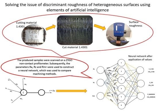
Solving the Issue of Discriminant Roughness of Heterogeneous Surfaces Using Elements of Artificial Intelligence


Faculty of Technology, Tomas Bata University in Zlín, Vavrečkova 275, 760 01 Zlín, Czech Republic
*
Author to whom correspondence should be addressed.
Materials 2021, 14(10), 2620; https://doi.org/10.3390/ma14102620
Submission received: 29 March 2021
/
Revised: 11 May 2021
/
Accepted: 14 May 2021
/
Published: 17 May 2021
(This article belongs to the Collection Additive Manufacturing: Alloy Design and Process Innovations)
Abstract
:This work deals with investigative methods used for evaluation of the surface quality of selected metallic materials’ cutting plane that was created by CO2 and fiber laser machining. The surface quality expressed by Rz and Ra roughness parameters is examined depending on the sample material and the machining technology. The next part deals with the use of neural networks in the evaluation of measured data. In the last part, the measured data were statistically evaluated. Based on the conclusions of this analysis, the possibilities of using neural networks to determine the material of a given sample while knowing the roughness parameters were evaluated. The main goal of the presented paper is to demonstrate a solution capable of finding characteristic roughness values for heterogeneous surfaces. These surfaces are common in scientific as well as technical practice, and measuring their quality is challenging. This difficulty lies mainly in the fact that it is not possible to express their quality by a single statistical parameter. Thus, this paper’s main aim is to demonstrate solutions using the cluster analysis methods and the hidden layer, solving the problem of discriminant and dividing the heterogeneous surface into individual zones that have characteristic parameters.
1. Introduction
The surface quality of the solid material determines and expresses both the grade of the workpiece and the product. Wood and stone products already require a certain level of surface quality for further use. Requirements on it are intensified with the development of metallurgy, especially in the production of cutting tools for daily use, e.g., knives, swords, sickles, scythes, and tools. However, in the production of these types of tools, the evaluation of the surface by sight or touch has been sufficient [1].
Machining methods have also been evolving, ranging from downright primitive to the traditional methods used to date, along with methods for classifying surface quality determination [1,2]. The roughness began to be prescribed in the blueprint and was given by standards that became documents approving the rules of product reproducibility. The “measurement” of surface roughness by sight and touch was no longer sufficient because it could not be measured accurately and precisely enough. With the advent of new technologies and modern measuring instruments, it was possible to measure the surface roughness and determine its parameters more accurately [1,2]. These technical possibilities were reflected in the standardization process [2].
The methods of surface quality evaluation prescribed by the standards and the repeatability of the production process have led to the idea that it is possible to determine the type of material to be machined under the conditions of repeatability of the measured roughness parameters. The subject of this work was to verify this idea [3,4].
The need for standardization of parts, products, and processes in industrial production is almost as old as industrial production itself. However, as globalization increases, the importance of interchangeability and substitutability within the supplier–customer chain increases. Setting up rules for assessing different products or production processes is the main goal of the International Organization for Standardization. Standardization in surface quality assessment is mainly dealt with in ISO 4287 and ISO 4288 [2].
Therefore, the article’s aim, considering the previous introduction, is to independently evaluate the surfaces that have arisen as a result of applying a water jet and laser beam to the aforementioned surfaces [5]. Due to the energy loss during the passage, when the cutting is carried out, the quality of the cut surface changes, which can be described by the roughness or waviness parameters, both in 2D and 3D [2].
Therefore, it is clear that this is a classical discriminatory task that methods of discrimination or cluster analysis can solve. However, in this case, the main responsibility for the solution is transferred from the metrologist to the statistician, which may be convenient for scientific but not practical application [6].
Normally, this problem is solved by evaluation of only the Ra parameter. Unfortunately, it has been confirmed several times that the parameter Ra itself is not sufficiently indicative of the surface quality. Therefore, the amplitude parameters Rz and the hybrid parameter Rmr(c) were added to the neural network [7].
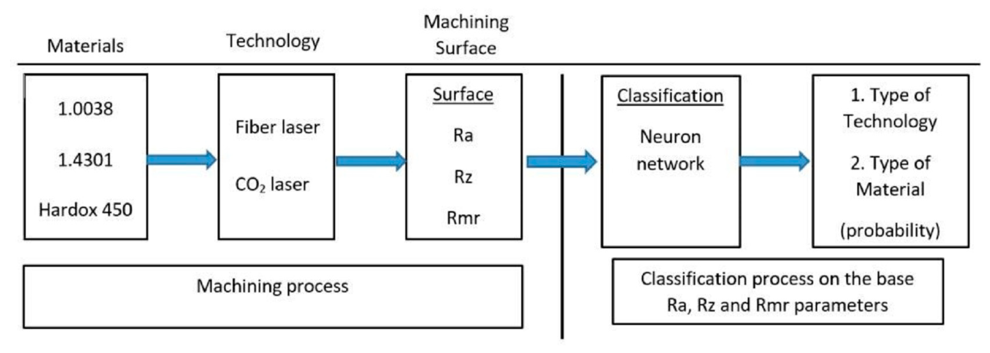
The novelty of this article lies in the possibility of comparing the roughness of surfaces created by two different machining methods by using a neural network. The surface quality expressed by Rz and Ra’s roughness parameters is examined depending on the sample material and the machining technology that was used [1,2]. The next part deals with the use of neural networks to evaluate measured data. In the last part, the measured data were statistically evaluated [2,8]. Based on the conclusions of this analysis, the possibilities of using neural networks to determine the material of a given sample with known roughness parameters were evaluated [8].
The suitability of using the perceptron neural networks with one hidden layer for this exact purpose will be described in the article. The suitability of using the perceptron neural networks with one hidden layer for this exact purpose will be described in the article. By creating a suitable file containing learning information for the neural network and finding a suitable number of neurons in a hidden layer, it is possible to apply it to solve the discriminatory task and, more precisely, find individual parameters [9,10].
2. Materials and Methods
2.1. Studied Materials and Their Machining
Three types of materials were used for the measurements, namely structural steel 1.0038- S235JRC + N (sample 235), abrasion-resistant stainless steel HARDOX 450 (sample HARDOX), and stainless steel 1.0043-X5CrNi18-10 (sample 1_430).
2.2. Surface Quality
During machining, surface irregularities arise due to the production technology. The quality of the surface and the associated roughness directly depend on the modifying method. To make surfaces comparable in quality, ISO 4287, ISO 4288, ISO 25178, and other norms define a number of parameters that can be used in other to quantify the surface of an observed sample [11].
This article presents parameters concerning surface roughness, i.e., R parameters, which were measured by Talysurf CLI 500 profilometer (Taylor & Hobson, Leicester, United Kingdom). These parameters include Ra—Arithmetical mean of height and Rz—Maximum height of profile. Furthermore, one hybrid parameter, Rmr (c)—Load length ratio of profile curve elements to the evaluation length at cut level c (% or µm), was used [1,5].
Before the roughness was measured on a Talysurf profilometer, the machined-surface areas were checked on a Leica optical microscope with a magnification of 50×. This control is necessary for the prevention of errors in the measurement itself. ISO 4287 clearly specifies that surface damage cannot be assessed.
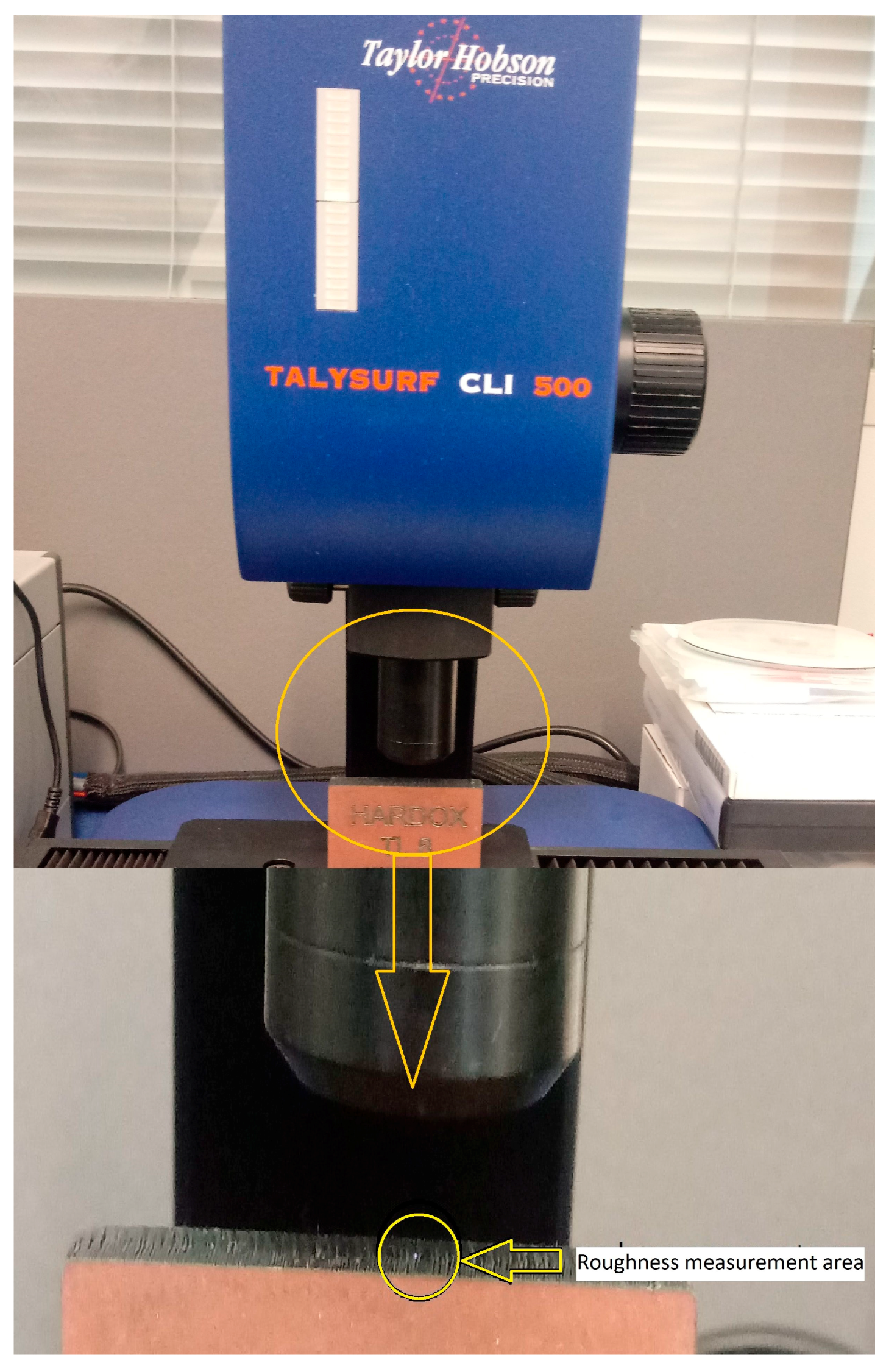
The measurement was performed under laboratory measurement conditions (temperature: 22 °C, atmospheric pressure: 1045 hPa) on a Talysurf CLI 500 profilometer (Figure 1). From three materials and two types of machining, six samples were produced. For each sample, 160 cuts were done on the X-axis and 280 on the Y-axis. The disproportion in the performed cuts is given by ISO 4277, where the main emphasis is placed on the X-axis as the central axis.
The following scanning parameters on the Talysurf CLI 500 profilometer were set: intensity reflection in the range of 85–95% (stabilization of the Z-axis), measurement speed 50 µm/s, and measurement spacing 5 µm on X and Y axes. Figure 1 shows the Talysurf profilometer with the marked measuring area.
2.3. Statistical Tools for Data Evaluation
On a theoretical level, surface quality is assessed by using a parameter that is given by ISO 4287 and ISO 25178 standards, and conclusions are drawn from statistical tests and analyses. These tests are standard statistical hypothesis tests, based on the assumption that the data from the scanned surface show a normal distribution and can be neglected [8,12]. Furthermore, the effect of systematic errors is not considered. Therefore, data analysis is carried out first to determine the type of distribution, deviations, skewness, and sharpness. The arithmetic mean and variance are mainly evaluated for parameters of the dataset [13,14].
2.4. Data Classification
In assessing the measurement data from a plurality of samples, data must be split into several subsets according to specific criteria. This identifies groups that show some similarity [8,12]. The division of data into groups is a part of the “statistical learning” discipline, where, based on a set of so-called training data, a prediction model is established. This allows a prediction of the output value with a certain probability. Further described is the use of neural networks to precisely determine the resulting values based on the input measurement data and cluster analysis method [9,12].
Clustering is one of the multidimensional data analysis techniques nowadays frequently used in artificial intelligence. The basic idea of the method is to divide the measured data into clusters, so the items from one cluster have “more similar” properties than others [1,14]. Furthermore, this approach is based on the evaluation of measured parameters (Ra, Rz, and Rmr) of samples’ surfaces (F_1_430, F_235, HARDOX) that were machined by laser technology CO2 and fiber [6,8].
For this distribution, the approach by Ward that is capable of finding the nearest clusters by optimizing distances of individual clusters was used. The optimization is based on finding the correlation coefficients that are linear scale distances [8,15].
The correlation coefficient used in the article expresses the mutual linear relationship between two quantities describing the quality of a surface. Then, the degree of correlation is expressed by the Pearson correlation coefficient, which can take values in the closed interval ranging from −1 to +1. A value close to +1 (−1) means that the linear relationship between two quantities is “very probable”. Using cluster analysis, it is possible to demonstrate that two (or more) clusters are “more probable” than the others [8,15].
2.5. Mathematical Model of the Neuron
In principle, the neuron is a unit that performs the representation of Euclidean space on real numbers {R}n –> R. This means that it converts n inputs to which weights are assigned to one output function value. The neuron output is a value ϒ; which is a function; designated as:
where is the intrinsic potential of a neuron. This function is calculated when the sum of the product value input xi × wi exceeds a predetermined value θ called the threshold. Figure 2 shows the principle of a neuron [3,4,13].
The transfer function can be divided into two categories. It is either a leap, i.e., the value of the output changes abruptly when the threshold is exceeded, or analogue, i.e., the continuous transfer function generates the output value. The jump function is only used for the output layer when binary output is required. For other layers, analogy functions are used [4,11].
One neuron itself can perform only the most basic operations. On the contrary, a structure of neurons can perform complex decision-making operations. These structures are known as neural networks. Thus, a neural network is an oriented graph with input, output, hidden nodes, and rated edges representing the signal flow [1,2].
Separate neurons are located in individual nodes. Nodes, their deployment, and interconnections are critical aspects of the network architecture. Input nodes mostly only distribute incoming data to all the first hidden layer’s neurons. Furthermore, the network may consist of several hidden layers designed to perform the desired operations as a whole. The output layer acts mainly as a network output interface [5,6,13].
3. Results and Discussion
3.1. Materials
3.2. Evaluation of Surface Roughness
As described above, the samples were cut by two types of lasers. First, it was necessary to check the surface on a microscope for defects that prevented a correct roughness assessment.
Figure 4 shows a section of material 1.0038 (6 mm and 8 mm thickness) machined by the fiber laser and CO2 laser. As is evident from the figure, the CO2 machining left a more apparent mark, while the surface of the sample cut with the fiber laser was smoother.
Figure 5 shows a section of material 1.4301 (6 mm and 8 mm thickness) machined by the fiber laser and CO2 laser. The general roughness of sections displayed on this figure is higher than on the previous one. Nevertheless, the surface left by the fiber laser is still smoother than the surface left by the CO2 laser. In addition, Figure 5D shows the evidence of the material being melted during the cutting procedure, which could be caused by the higher concentration of nickel in this material.
Figure 6 shows a section of material Hardox 450 (6 mm and 8 mm thickness) machined by the fiber laser and CO2 laser. While the previous two materials had a smoother section surface after being cut by a fiber laser, an opposite trend was observed in samples prepared from HARDOX 450. This might have been caused by the high abrasion resistance of this material.
Figure 7 graphically compares the surfaces of material 1.0038. Figure 7A shows a section of material (6 mm thickness) machined by the fiber laser. Figure 7B shows a section of material (8 mm thickness) machined by the fiber laser, too. Figure 7C shows a section of material (6 mm thickness) machined by the CO2 laser. Figure 7D shows a section of material (8 mm thickness) machined by the CO2 laser, too. All surfaces are characterized by triple parameters (Ra, Rz, Rmr) that change with the varying measuring position. Examples of measured triplets can be found in Table 5.
Figure 8 graphically compares the surfaces of material 1.4301. Figure 8A shows a section of material (6 mm thickness) machined by the fiber laser. Figure 8B shows a section of material (8 mm thickness) machined by the fiber laser. Figure 8C shows a section of material (6 mm thickness) machined by the CO2 laser. Figure 8D shows a section of material (8 mm thickness) machined by the CO2 laser. All surfaces are characterized by triple parameters (Ra, Rz, Rmr) that change with the varying measuring position. Examples of measured triplets can be found in Table 5.
Figure 9 graphically compares the surfaces of material Hardox 450. Figure 9A shows a section of material (6 mm thickness) machined by the fiber laser. Figure 9B shows a section of material (8 mm thickness) machined by the fiber laser. Figure 9C shows a section of material (6 mm thickness) machined by the CO2 laser. Figure 9D shows a section of material (8 mm thickness) machined by the CO2 laser. All surfaces are characterized by triple parameters (Ra, Rz, Rmr) that change with the varying measuring position. Examples of measured triplets can be found in Table 5.
As shown by the figures presented above, the quality of the surfaces of individual materials machined by individual types of lasers is highly variable. In practice, this variability is called a heterogeneous surface. These surfaces are characterized by the fact that the above parameters Ra, Rz, and Rmr show considerable variance. Therefore, it is quite difficult to use classical statistical methods for their recognition and subsequent classification. Therefore, a cluster analysis capturing the similarity of the above-mentioned heterogeneous surfaces seems to be a suitable method.
3.3. Statistical Evaluation
The first step of the statistical evaluation of the measured parameters Ra and Rz of the surfaces of materials 1.0038, 1.4301, and Hardox 450, machined with fiber laser and CO2 laser technology, was to perform the Anderson Darling test of normality at the confidence level of 95%. A two-way Grubs test followed this to rule out the possibility of data infiltration by gross errors.
Figure 10 shows the graphs clearly showing that Ra and Rz variances depend on the used machining technology and the material itself.
For this reason, cluster analysis was applied to demonstrate the similarity of materials and technologies. However, it seems to be much more appropriate for the classification process to use a neural network, which will perform its classification separately after proper “learning” (see Figure 11).
3.4. Classification of Evaluated Data and Cluster Analysis
This data analysis step was designed to determine if the data showed any similarity and, if so, to describe this similarity in detail [15]. Since the possibility of determining the material used by the measured roughness parameters was examined, only samples processed with the same technology were compared. For the actual analysis, the recommended Ward’s method was used for the formation of clusters [16].
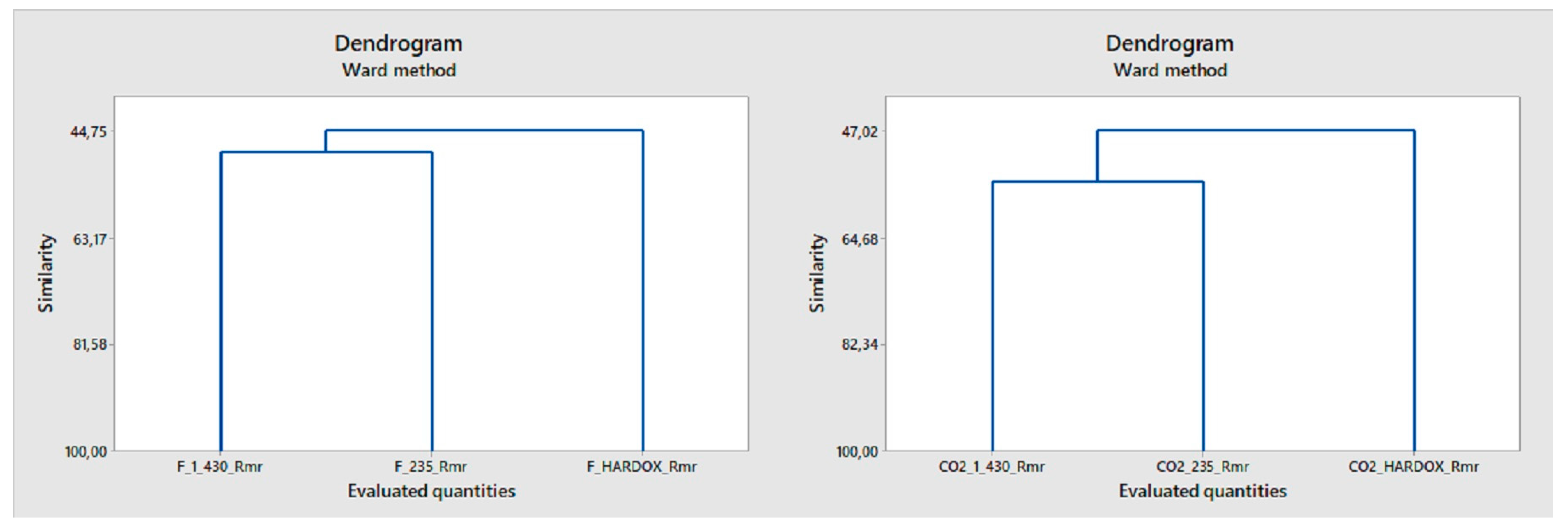
As shown by the dendrograms in Figure 12 and Figure 13, three different sheets of steel, namely 1.0043, 1.0038, and Hardox 450, having a heterogeneous surface resulting from their cutting by two types of lasers, namely a fiber and CO2 laser, were considered [17]. The purpose was to find a mutual similarity in terms of discriminant surfaces using the amplitude parameters Ra and Rz. Then, this similarity was numerically expressed using the Pearson correlation coefficient; see Table 3 and Table 4. As expected, F Hardox steel exhibited maximum dissimilarity across clusters [18].
However, the same task is, as it is demonstrated below, was solved more accurately using a single hidden layer neural network where there is no limitation of the linearity given by the Pearson correlation coefficient [19]. Moreover, the amplitude parameters cannot capture the heterogeneous surface property; therefore, it is necessary to add another hybrid parameter (in the sense of ISO 4287), namely Rmr(c), to the inputs of the searched and subsequently tune the neural network [1,6].
In Table 3 and Table 4, the levels of similarity of fiber and CO2 laser-treated samples using Pearson’s correlation coefficient are shown:
This method does not recognize the difference in the cluster of steels 1.0043 and 1.0038 well, so it is necessary to add another discriminatory parameter, the hybrid parameter Rmr (Figure 14).
3.5. Neuron Network
Tests have shown that the two materials always have roughness parameters similar to those for which it is not possible to determine a material with sufficient reliability only based on the measured Rz and Ra values. Therefore, the next decision was to consider determining parameter Rmr according to the ISO 4288 norm. For the determination of similarity, we designed a neural network using an adaptation algorithm with one hidden layer.
Software Statistica 14.0 was used to build the neural network. First, the number of neurons in the hidden layer was estimated according to the formula: [1,2]
where:
- NNH is the number of neurons in the hidden layer
- n1 is the number of neurons in the input layer
- n2 is the number of neurons in the output layer
To prove the correct functionality of the learned neural network, 30 samples machined with the described technologies were selected. For these samples, the three parameters Rz, Ra, and Rmr were measured in any position. These parameters are entered at the input of the demonstrated neural network, which performed its classification process and calculated the probability of this classification.
From Table 5, it can be concluded that the probability of most classifications exceeds 90% for materials machined with fiber laser. In the case of materials machined with a CO2 laser, the triple scattering values result in a lower value of the probability of classification; however, in most cases, it exceeds 60%, which can be considered satisfactory. Should this probability need to be increased, further learning of the neural network would need to be continued.
For each type of machining technology used, a neural network was constructed and tested on a training dataset. This set contained 753 ordered triplets [Rz; Ra; Rmr], which were the measured values of these roughness parameters on all samples machined in the same way. Then, these triplets were inserted at the input of the appropriate neural network, which performed its recognition of the type of material and laser machining technology. The neural network was debugged in the environment of Statistica 14.0 software, specifically in the neural network part.
In order to use this neural network without software Statistica 14.0, C ++ source code was generated using the scales, and the neural networks were further tested with a free Dev C ++ development environment. Based on this theoretical estimate, the neural network would look as suggested in Figure 15.
Both neural networks recognized the material correctly, even though the CO2 laser sample evaluation neural network showed a lower probability of a correct decision due to a lower level of learning. Hence, a higher error formula value was lying on the error plane.
Based on measurements of individual heterogeneous surfaces of sample materials defined in Table 5 machined with two types of lasers, a database containing 753 arranged triplets, specifically a pair of amplitude parameters Ra and Rz and one hybrid Rmr parameter, was manually created.
This was used to teach the creation of a three-input neural network and with one hidden layer. The optimum number has been optimized by the number 6, which comes from Figure 15 and constitutes the best solution for discrimination, and it is also the network’s output. The result of such discriminant is the specification of the cutting technology on the sample material in any scanned cut of the heterogeneous surface.
As shown in Table 3 and Table 4, the probability of distinguishing the cutting technology from the sample material and the sensing position is rarely below the probability of 85% recognition for the fiber laser and all types of unknown sample materials.
In the case of a CO2 laser, the situation is more complicated. The probability of recognition may decrease to 50% for measured unknown samples, which is extreme. In general, samples cut by fiber laser technology have a much higher probability of correct recognition than samples cut by CO2 laser, which is mainly due to the different typology of cutting [9,10].
4. Conclusions
The main idea of this work was to show the use of the measured values of roughness parameters to determine the sample material using artificial intelligence elements. First, Rz, Ra, and Rmr parameter values were acquired for each sample using the Talysurf CLI500 3D scanner. The measured data were first analyzed by Minitab version 18. It was verified whether the data contained outliers or whether gross measurement errors influenced them in several steps. After that, the sets of values of Rz and Ra’s parameters were analyzed for a statistically significant influence on the material or technology used. In all cases, the influence of the material and the machining technology applied was found to be statistically significant. In the next step, data were sorted by similarity criteria using cluster analysis. Since the two sets of data always shown high similarity, it turned out that using only the parameters Rz and Ra in combination with standard statistical analysis procedures was not sufficient to determine the sample material. Therefore, for each laser type, Statistica 14.0 generated a perceptron neural network with one hidden layer, which evaluated the measured values of the parameters as mentioned above together with the values of the parameter Rmr, which was used as an additional criterion in the determination of the sample. Then, these networks were tested on a test dataset, and in all cases, the material was correctly recognized by the network.
In general, the fiber laser sample network showed higher reliability than the CO2 laser sample network. The highest reliability was recorded for fiber laser-treated steel 1.0043 and the lowest was recorded for CO2 laser-treated steel 1.0043.
When comparing the results contained in this article, it can be stated that the evaluation of heterogeneous surfaces of samples based on the parameters of ISO 4287 and ISO 25178 standards cannot be done well without using discriminatory statistical methods.
However, even today’s commonly used cluster analysis in this assessment may fail or give distorted and inexact results if clustering is based on Pearson coefficients, as described in the article and the relevant tables.
Unambiguously, the best but not the most uncomplicated method seems to be the use of artificial intelligence elements, namely the classical three-input neural network, with one hidden layer containing six neurons, performing its solution to the discriminatory problem in cutting technology and sample material having a heterogeneous surface.
In the case of high-quality sorted data containing triples of amplitude and hybrid parameters, the so-called learning of the found neural network, as described in the article, can be realized according to the triplets describing the character of heterogeneous surfaces in arbitrary sections. As shown from the results table, a well-learned neural network, one with minimized error function, can indicate a low probability of discriminant in various cutting technologies and complicated heterogeneous surfaces.
Then, it depends on whether it is possible to create separate networks for individual technologies, which is understandably more likely to be discriminatory, but at the expense of significantly complicating the solution or a universal network, as demonstrated in this article.
Author Contributions
Methodology, Project administration, Writing—Original Draft, M.K.; Conceptualization, Validation, V.P.; Funding acquisition, Writing—Review & Editing, D.M.; Visualization, Resources, Investigation, A.Š.; Data Curation, Software, M.M. All authors have read and agreed to the published version of the manuscript.
Funding
This research received no external funding.
Institutional Review Board Statement
Not applicable.
Informed Consent Statement
Not applicable.
Data Availability Statement
The data presented in this study are available on request from the corresponding author.
Acknowledgments
This article was written with the support of the project IGA/FT/2021/006 TBU in Zlín. The authors would like to thank student Radek Zaoral for their cooperation.
Conflicts of Interest
The authors declare no conflict of interest.
References
- Whitehouse, D.J. Handbook of Surface and Nanometrology, 2nd ed.; CRC Press: London, UK, 2011. [Google Scholar]
- Murat, D.; Ensarioglu, C. Surface Roughness Analysis of Greater Cutting Depths During Hard Turning. Mater. Test. 2017, 59, 795–802. [Google Scholar] [CrossRef]
- Fu, G.; Sun, P.; Zhu, W.; Yang, J.; Cao, Y.; Yang, M.; Cao, Y. A Deep-Learning-Based Approach for Fast and Robust Steel Surface Defects Classification. Opt. Lasers Eng. 2019, 121, 397–405. [Google Scholar] [CrossRef]
- Yida, L.; Gao, T. Local Defects in Colloidal Quantum Dot Thin Films Measured Via Spatially Resolved Multi-Modal Optoelectronic Spectroscopy. Adv. Mater. 2020, 31, 105–119. [Google Scholar]
- Patel, A.; Bhavsar, S.N. Experimental investigation to optimize laser cutting process parameters for difficult to cut die alloy steel using response surface methodology. Mater. Today Proc. 2021, 43, 28–35. [Google Scholar] [CrossRef]
- Giudice, F.; Missori, S. Parameterised multipoint-line analytical modeling of a mobile heat source for thermal field prediction in laser beam welding. Int. J. Adv. Manuf. Technol. 2021, 112, 1339–1358. [Google Scholar] [CrossRef]
- Neslušan, M.; Minárik, P. Non-destructive evaluation of the railway wheel surface damage after long-term operation via Barkhausen noise technique. Wear 2019, 420–421, 195–206. [Google Scholar] [CrossRef]
- Abonyi, J.; Feil, B. Cluster Analysis for Data Mining and System Identification, 1st ed.; Birkhäuser Basel: Basel, Switzerland, 2007. [Google Scholar]
- Yadav, N.; Yadav, A. An Introduction to Neural Network Methods for Differential Equations; Springer: Berlin/Heidelberg, Germany, 2015. [Google Scholar]
- Patterson, D.W. Artificial Neural Networks: Theory and Applications; Prentice Hall: New York, NY, USA, 1996. [Google Scholar]
- Muthuramalingam, T.; Akash, R. Surface quality measures analysis and optimization on machining titanium alloy using CO2 based laser beam drilling process. J. Manuf. Process. 2021, 62, 1–6. [Google Scholar] [CrossRef]
- Mayuet Ares, P.; Vázquez Martínez, J. Experimental Study of Macro and Microgeometric Defects in Drilled Carbon Fiber Reinforced Plastics by Laser Beam Machining. Materials 2018, 11, 1466. [Google Scholar] [CrossRef] [PubMed] [Green Version]
- Patel, A.R.; Bhavsar, S.N. Laser Machining of Die Steel (EN-31): An. Experimental Approach to Optimize Process. Parameters using Response Surface Methodology. Int. J. Automot. Mech. Eng. 2021, 18, 8563. [Google Scholar] [CrossRef]
- Kumar, U.; Gope, D. Experimental and Numerical Assessment of Temperature Field and Analysis of Microstructure and Mechanical Properties of Low Power Laser Annealed Welded Joints. Materials 2018, 11, 1514. [Google Scholar] [CrossRef] [PubMed] [Green Version]
- Domokos, E.-K.; Bálint, C. Definition of user groups applying Ward’s method. Transp. Res. Procedia 2017, 22, 25–34. [Google Scholar]
- Erdenechimeg, K.; Jeong, H.-I. A Study on the Laser-Assisted Machining of Carbon Fiber Reinforced Silicon Carbide. Materials 2019, 12, 2061. [Google Scholar] [CrossRef] [PubMed] [Green Version]
- Callus, E.; the Approach-IS consortium and the International Society for Adult Congenital Heart Disease (ISACHD); Pagliuca, S.; Boveri, S.; Ambrogi, F.; Luyckx, K.; Kovacs, A.H.; Apers, S.; Budts, W.; Enomoto, J.; et al. Phenotypes of adults with congenital heart disease around the globe: A cluster analysis. Health Qual. Life Outcomes 2021, 19, 1–10. [Google Scholar] [CrossRef] [PubMed]
- Guarino, S.; Ponticelli, G.S. Environmental assessment of Selective Laser Melting compared with Laser Cutting of 316L stainless steel: A case study for flat washers’ production. CIRP J. Manuf. Sci. Technol. 2020, 31, 525–538. [Google Scholar] [CrossRef]
- Quondam Antonio, S.; Riganti Fulginei, F. An effective neural network approach to reproduce magnetic hysteresis in electrical steel under arbitrary excitation waveforms. J. Magn. Magn. Mater. 2021, 528, 167735. [Google Scholar] [CrossRef]
Figure 1.
Profilometer Talysurf CLI 500.

Figure 2.
Basic principle of neuron.

Figure 3.
Material cut 1.4301 (A), CO2 laser, (B) Fiber laser.

Figure 4.
Material cuts 1.0038: (A) 6 mm fiber laser, (B) 8 mm fiber laser, (C) 6 mm CO2 laser, (D) 8 mm CO2 laser.
Figure 4.
Material cuts 1.0038: (A) 6 mm fiber laser, (B) 8 mm fiber laser, (C) 6 mm CO2 laser, (D) 8 mm CO2 laser.

Figure 5.
Material cuts 1.4301: (A) 6 mm fiber laser, (B) 8 mm fiber laser, (C) 6 mm CO2 laser, (D) 8 mm CO2 laser.
Figure 5.
Material cuts 1.4301: (A) 6 mm fiber laser, (B) 8 mm fiber laser, (C) 6 mm CO2 laser, (D) 8 mm CO2 laser.

Figure 6.
Material cuts Hardox 450: (A) 6 mm fiber laser; (B) 8 mm fiber laser, (C) 6 mm CO2 laser; (D) 8 mm CO2 laser.
Figure 6.
Material cuts Hardox 450: (A) 6 mm fiber laser; (B) 8 mm fiber laser, (C) 6 mm CO2 laser; (D) 8 mm CO2 laser.

Figure 7.
Comparison of 3D scenes of materials 1.0038 section surfaces profilometer.

Figure 8.
Comparison of 3D scenes of materials 1.4301 section surfaces profilometer.

Figure 9.
Comparison of 3D scenes of materials Hardox 450 section surfaces profilometer.

Figure 10.
Demonstration of dispersion measuring parameters.

Figure 11.
Procedure of classification process using neural network.

Figure 12.
Cluster analysis of samples processed by fiber laser parameters Rz and Ra.

Figure 13.
Cluster analysis of samples processed by CO2 laser parameters Rz and Ra.

Figure 14.
Cluster analysis of samples processed by fiber laser and CO2 laser parameter Rmr.

Figure 15.
Perceptron with six hidden neurons.


Table 1.
The laser settings during sample production.
| Machining Type | Material Type | Material Thickness [mm] | Cutting Gas | Gas Pres. [Bar] | Cutting Jet Diam. [mm] | Focal Length [mm] | Cutting Speed [mm min−1] | Power [W] |
|---|---|---|---|---|---|---|---|---|
| Fiber laser | 1.0038 | 6 | Oxygen | 0.73 | 1.2 | 4.4 | 2600 | 3080 |
| Fiber laser | 1.0038 | 8 | Oxygen | 0.5 | 1.2 | 4 | 1700 | 3050 |
| Fiber laser | Hardox | 6 | Oxygen | 0.73 | 1.2 | 4.4 | 1300 | 3080 |
| Fiber laser | Hardox | 8 | Oxygen | 0.5 | 1.2 | 4 | 900 | 3050 |
| Fiber laser | 1.4301 | 6 | Nitrogen | 17 | 2.5 | −5.7 | 2100 | 3080 |
| Fiber laser | 1.4301 | 8 | Nitrogen | 19.3 | 2.5 | −7.3 | 1200 | 3080 |
| CO2 laser | 1.0038 | 6 | Oxygen | 0.7 | 1 | 0.7 | 2700 | 4000 |
| CO2 laser | 1.0038 | 8 | Oxygen | 0.4 | 1.5 | 1.5 | 2100 | 4000 |
| CO2 laser | Hardox | 6 | Oxygen | 0.7 | 1 | 0.7 | 2700 | 4000 |
| CO2 laser | Hardox | 8 | Oxygen | 0.4 | 1.5 | 1.5 | 2100 | 4000 |
| CO2 laser | 1.4301 | 6 | Nitrogen | 13 | 2 | −6.5 | 1350 | 4000 |
| CO2 laser | 1.4301 | 8 | Nitrogen | 14 | 2.5 | −9 | 1000 | 4000 |
Table 2.
Marking of measured samples.
| Indication | Pattern |
|---|---|
| F_1_430 | steel 1.0043 Fiber laser machining |
| CO2_1_430 | laser-treated CO2 steel 1.0043 |
| F_235 | steel 1.0038 Fiber laser machining |
| CO2_235 | laser-treated CO2 steel 1.0038 |
| F_HARDOX | steel HARDOX 450 Fiber laser machining |
| CO2_HARDOX | laser-treated CO2 steel HARDOX 450 |
Table 3.
Similarity levels of fiber laser-treated samples.
| Cluster | F_1_430 | F_235 F_HARDOX |
|---|---|---|
| Similarity Levels [%] | Similarity Levels [%] | |
| Rz | 67.3 | −1.05 |
| Ra | 71.5 | −9.3 |
Table 4.
Similarity levels of laser-treated samples CO2.
| Cluster | CO2_1_430 | CO2_235 CO2_HARDOX |
|---|---|---|
| Similarity Levels [%] | Similarity Levels [%] | |
| Rz | 59.8 | 88.7 |
| Ra | 52.4 | 91.6 |
Table 5.
Proof of the functionality of the proposed neural network solving the classification problem.
Table 5.
Proof of the functionality of the proposed neural network solving the classification problem.
| Fiber Laser | CO2 Laser | ||||||||
|---|---|---|---|---|---|---|---|---|---|
| Rz [µm] | Ra [µm] | Rmr | Recognized | % | Rz [µm] | Ra [µm] | Rmr | Recognized | % |
| 20.30 | 4.80 | 0.60 | F_1_430 | 0.99850 | 13.40 | 2.60 | 0.62 | CO2_1_430 | 0.6122 |
| 18.50 | 4.60 | 1.80 | F_1_430 | 0.99980 | 11.30 | 2.50 | 1.80 | CO2_1_430 | 0.8978 |
| 20.32 | 4.70 | 1.20 | F_1_430 | 0.99850 | 11.90 | 2,52 | 1,86 | CO2_1_430 | 0,7229 |
| 20,98 | 4,78 | 2,40 | F_1_430 | 0,99820 | 11,70 | 2,54 | 1,24 | CO2_1_430 | 0,5873 |
| 19,40 | 4,48 | 3,10 | F_1_430 | 0,99820 | 12,40 | 2,40 | 1,20 | CO2_1_430 | 0.8348 |
| 20.40 | 4.90 | 1.80 | F_1_430 | 0.99900 | 11.60 | 2.10 | 0.60 | CO2_1_430 | 0.8873 |
| 19.20 | 5.00 | 2.40 | F_1_430 | 0.99930 | 10.70 | 2.12 | 0.62 | CO2_1_430 | 0.6611 |
| 21.80 | 5.20 | 1.80 | F_1_430 | 0.99910 | 11.40 | 2.62 | 1.80 | CO2_1_430 | 0.4669 |
| 22.27 | 5.60 | 0.60 | F_1_430 | 0.99940 | 11.20 | 2.43 | 0.62 | CO2_1_430 | 0.5175 |
| 21.20 | 5.20 | 1.20 | F_1_430 | 0.99920 | 11.60 | 2.30 | 0.62 | CO2_1_430 | 0.7579 |
| 7.50 | 1.40 | 3.70 | F_235 | 0.99998 | 8.70 | 1.40 | 1.80 | CO2_235 | 0.4242 |
| 6.80 | 1.30 | 3.70 | F_235 | 0.99998 | 5.00 | 1.20 | 13.60 | CO2_235 | 0.9849 |
| 6.70 | 1.26 | 1.20 | F_235 | 0.99940 | 7.30 | 1.44 | 4.30 | CO2_235 | 0.9134 |
| 6.60 | 1.41 | 1.24 | F_235 | 0.99270 | 6.20 | 1.10 | 3.70 | CO2_235 | 0.9307 |
| 6.20 | 1.25 | 0.60 | F_235 | 0.99880 | 7.50 | 1.40 | 3.10 | CO2_235 | 0.8222 |
| 7.20 | 1.31 | 1.86 | F_235 | 0.99970 | 6.70 | 1.30 | 3.00 | CO2_235 | 0.9085 |
| 5.90 | 1.20 | 8.07 | F_235 | 1.00000 | 6.00 | 1.10 | 3.70 | CO2_235 | 0.9419 |
| 6.00 | 1.42 | 3.10 | F_235 | 0.95950 | 6.60 | 1.20 | 0.60 | CO2_235 | 0.9165 |
| 7.20 | 1.49 | 1.20 | F_235 | 0.98950 | 7.10 | 1.18 | 2.50 | CO2_235 | 0.8538 |
| 6.95 | 1.41 | 0.60 | F_235 | 0.99640 | 6.30 | 1.22 | 8.00 | CO2_235 | 0.9607 |
| 13.30 | 2.60 | 0.62 | F_HARDOX | 0.88750 | 16.60 | 3.70 | 1.80 | CO2_HARDOX | 0.6329 |
| 11.20 | 2.50 | 1.86 | F_HARDOX | 0.99999 | 14.10 | 3.50 | 1.20 | CO2_HARDOX | 0.9273 |
| 11.90 | 2.52 | 1.80 | F_HARDOX | 0.99940 | 15.10 | 3.60 | 1.80 | CO2_HARDOX | 0.9074 |
| 11.80 | 2.54 | 1.24 | F_HARDOX | 0.99900 | 15.00 | 3.70 | 0.62 | CO2_HARDOX | 0.9745 |
| 12.40 | 2.41 | 1.24 | F_HARDOX | 0.86100 | 14.44 | 3.60 | 1.10 | CO2_HARDOX | 0.9728 |
| 11.40 | 2.10 | 0.62 | F_HARDOX | 0.87560 | 14.80 | 3.50 | 1.80 | CO2_HARDOX | 0.7229 |
| 10.80 | 2.12 | 0.62 | F_HARDOX | 0.99880 | 14.60 | 3.55 | 1.24 | CO2_HARDOX | 0.8973 |
| 11.50 | 2.62 | 1.80 | F_HARDOX | 0.99970 | 14.20 | 3.70 | 0.60 | CO2_HARDOX | 0.9937 |
| 11.29 | 2.40 | 0.60 | F_HARDOX | 0.99880 | 15.00 | 3.50 | 4.30 | CO2_HARDOX | 0.8853 |
| 11.64 | 2.30 | 0.62 | F_HARDOX | 0.99870 | 13.30 | 3.40 | 3.70 | CO2_HARDOX | 0.9415 |
Publisher’s Note: MDPI stays neutral with regard to jurisdictional claims in published maps and institutional affiliations. |
© 2021 by the authors. Licensee MDPI, Basel, Switzerland. This article is an open access article distributed under the terms and conditions of the Creative Commons Attribution (CC BY) license (https://creativecommons.org/licenses/by/4.0/).
Share and Cite
MDPI and ACS Style
Kubišová, M.; Pata, V.; Měřínská, D.; Škrobák, A.; Marcaník, M. Solving the Issue of Discriminant Roughness of Heterogeneous Surfaces Using Elements of Artificial Intelligence. Materials 2021, 14, 2620. https://doi.org/10.3390/ma14102620
AMA Style
Kubišová M, Pata V, Měřínská D, Škrobák A, Marcaník M. Solving the Issue of Discriminant Roughness of Heterogeneous Surfaces Using Elements of Artificial Intelligence. Materials. 2021; 14(10):2620. https://doi.org/10.3390/ma14102620
Chicago/Turabian StyleKubišová, Milena, Vladimír Pata, Dagmar Měřínská, Adam Škrobák, and Miroslav Marcaník. 2021. "Solving the Issue of Discriminant Roughness of Heterogeneous Surfaces Using Elements of Artificial Intelligence" Materials 14, no. 10: 2620. https://doi.org/10.3390/ma14102620
Note that from the first issue of 2016, this journal uses article numbers instead of page numbers. See further details here.