2.1. The Basic Concept of the Strain Intensity Factor
Irwin introduced the stress intensity factor Δ
K as a driving parameter of the crack propagation (based on the small yield assumption [
39]), while the SIF is defined as
where Δ
K represents the range of the stress intensity factor,
γ represents the geometrical coefficient,
a is the crack flaw size, and
is the stress range. The SIF is the function of the global stress and geometry of the specimen, which can describe the local stress field near the crack tip. So, the SIF becomes a major driving parameter to correlate with the crack growth rate by many researchers [
21,
22,
23]. However, some studies reveal that the strain intensity factor shows a better correlation with the crack growth for some materials under the fully reversed loading condition [
37]. In those experimental studies, the SIF cannot give a satisfactory performance. Therefore, a strain-intensity-factor-based method is proposed in this paper. Similar to the SIF, for the simplest case (mode–I) the strain intensity factor is defined as follows:
where
is the range of the strain intensity factor and
is the strain range.
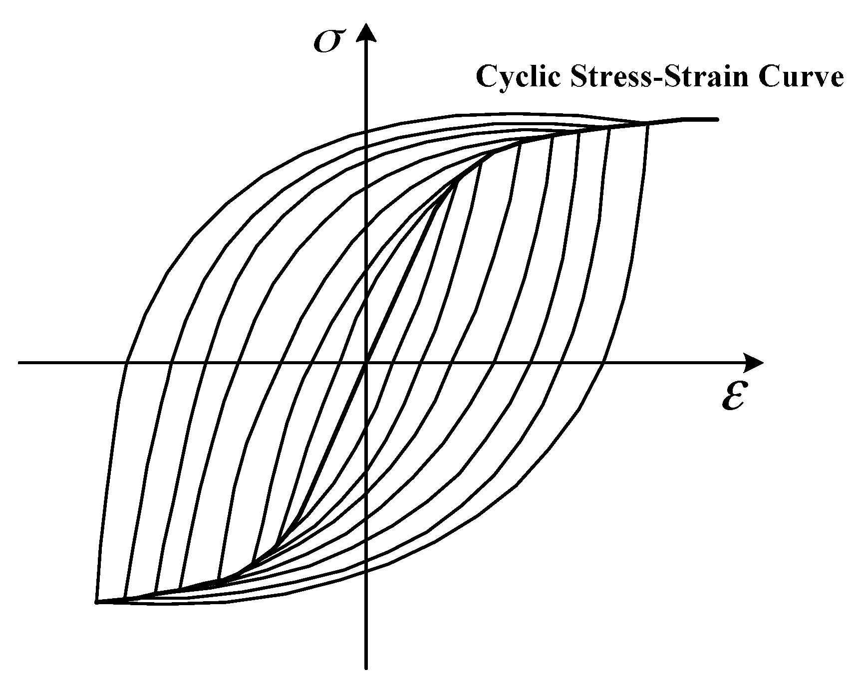
For the cyclic tension-tension load condition, the stress range and strain range vary linearly within the elastic region. For uniaxial, their relationship follows Hooke’s law, so the stress intensity factor and strain intensity factor are proportional. Therefore, the fatigue life predicted by the strain intensity factor should be the same as that obtained by using the SIF. However, for some materials under the tension-compression load condition, their cyclic stress and strain are not linearly related. The constitutive function should follow the cyclic stress-strain curve rather than the monotonic one (as shown in
Figure 1). It can be seen that increasing the applied loading range will give rise to a more severe nonlinearity, and the hysteresis loop range will become wider. The formula between the cyclic stress and strain proposed by Ramberg-Osgood is expressed as Equation (3) [
40]
where
is the total strain,
is the elastic strain,
is the plastic strain,
K′ represents the cyclic strength coefficient, and
n′ represents the cyclic strain hardening coefficient.
It is known that the flow bands at the crack tip will be activated under the cyclic tension-compression loading, which are induced by the dislocation movements. Crack propagation occurs when the accumulated cyclic strain exceeds the fracture strain [
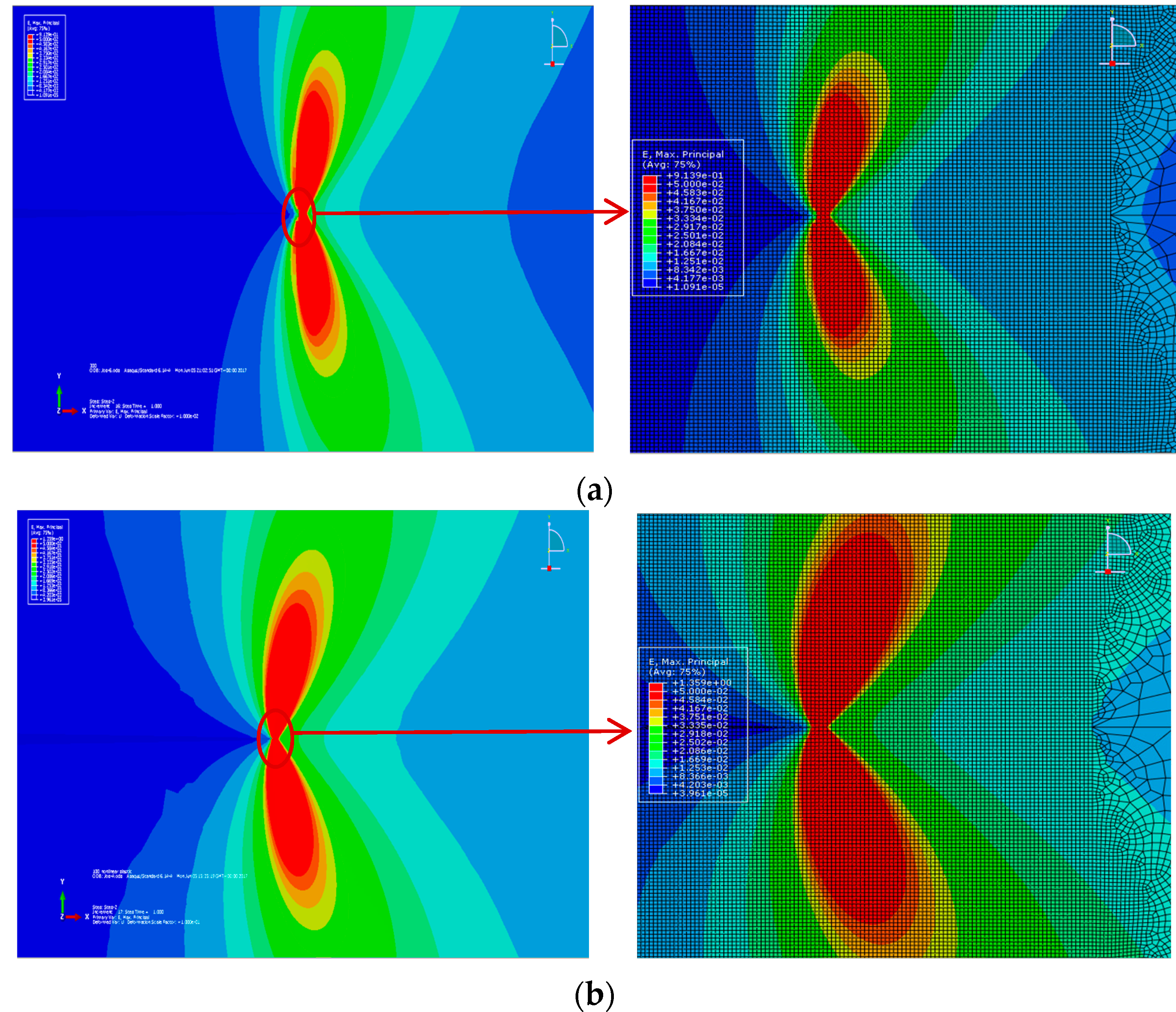
31]. So, the crack growth is more directly linked to the strain than to the stress. A 3D finite element simulation is conducted for a comparative demonstration. With the same geometry configuration and the applied stress range, different constitutive relationships will lead to a deviation of the global strain variation. Furthermore, the local strain fields at the crack tip are also quite different, which will ultimately influence the fatigue crack growth process. In
Figure 2, the difference of the strain fields at the crack tip is visualized by using the finite element (FE) software ABAQUS. In
Figure 2a,b the constitutive relationships follow the linear elastic and perfect plastic, and nonlinear cyclic stress-strain relationships respectively, which have an identical yield stress or 0.2% proof strength. The mechanical properties of the materials in the FE analysis are listed in
Table 1.
The 0.2% proof strength of the material is 297 MPa; Young’s modulus and Poisson’s ratio are 202.5 GPa and 0.3 respectively. The cyclic strength coefficient and cyclic strain hardening coefficient are 691 and 0.154, while the applied loading is 200 MPa.
The simulation results of the remote strain and maximum local strain at the crack tip (for these two constitutive equations) are listed in
Table 2. As seen in
Table 2, under the same applied loading, the remote strain calculated by the nonlinear cyclic stress-strain relationship is larger than the linear elastic and perfect plastic one by 25.2%. The relative difference of the maximum local strain at the crack tip is 31.9%. It indicates that for some materials the strain range is a better parameter to describe the crack growth than the stress range.
Thus the relationship between the SIF range and the strain intensity factor range is also nonlinear in this condition. According to Equations (2) and (3), the formulation of the strain intensity factor under the fully reversed loading condition is proposed, which can be expressed as:
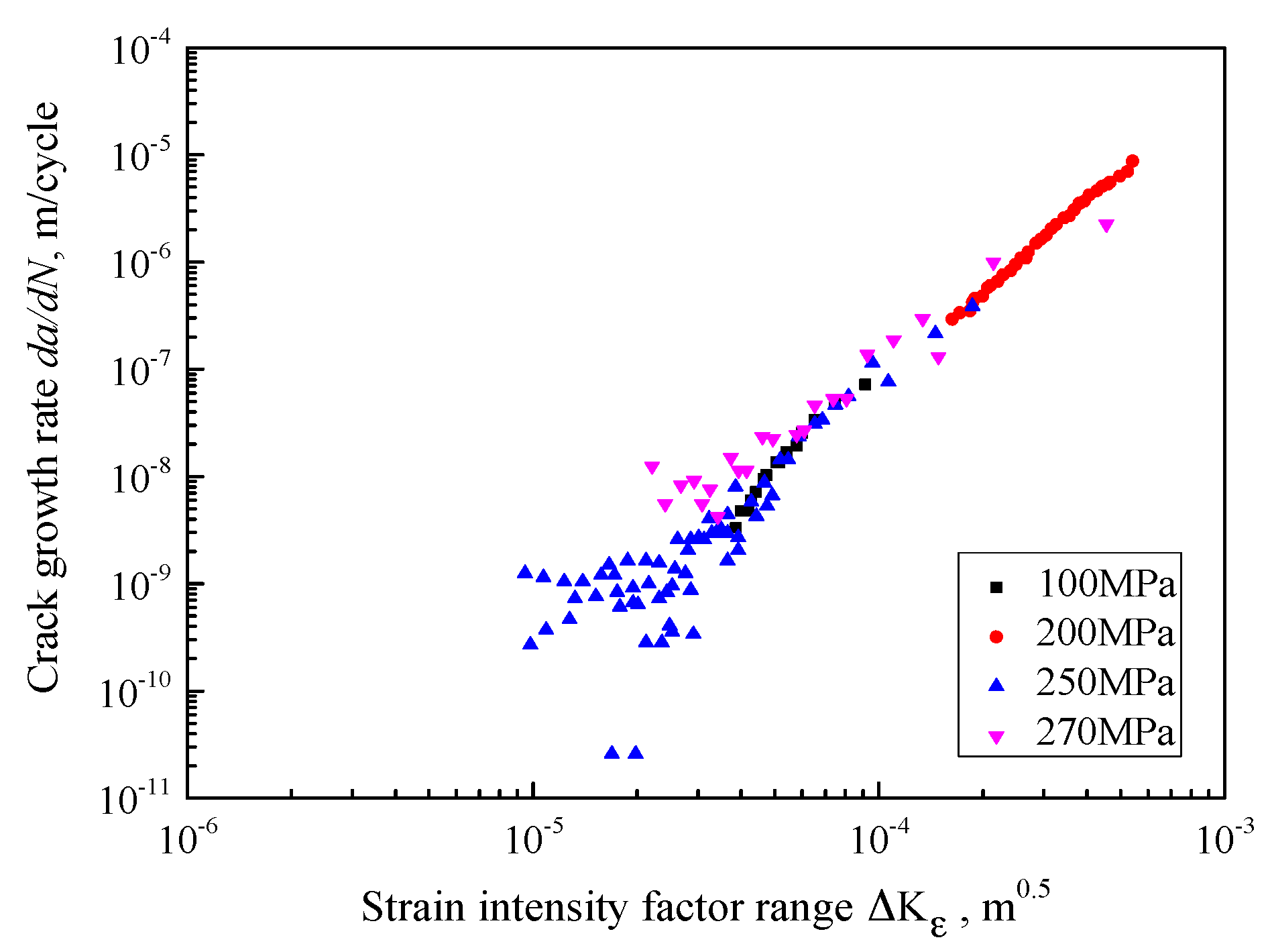
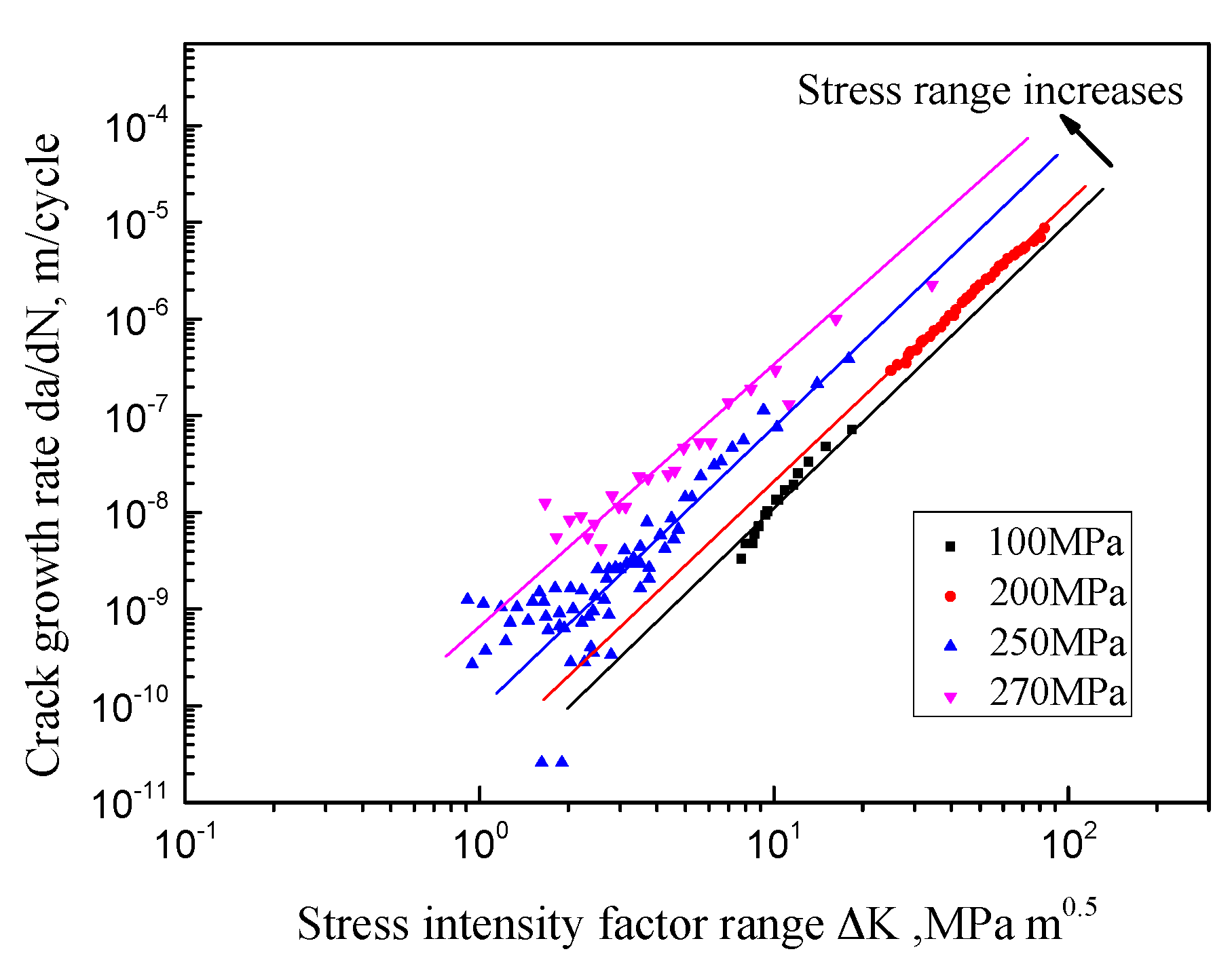
To illustrate the difference between the SIF and the strain intensity factor in the correlation with the crack growth rate, the crack growth data in 316 stainless steel (under the fully reversed loading with different stress ranges) is analyzed. As shown in
Figure 3, the lateral horizontal axis represents the SIF range and the vertical axis represents the crack growth rate. The dots in different shapes and colors represent the experimental measurements under different stress ranges. And all the data are from the fully reversed fatigue testing of cylindrical specimens in 316 stainless steel. Based on the traditional SIF method, all the testing data should shrink into one straight line, because of the same R-ratio. However, the testing data of different stress ranges follow several parallel straight lines. As shown in
Figure 3, the lines in different colors represent the trends of the testing data under different stress levels. Distinct deviations are observed between the different groups of these data. Moreover, fixing the SIF range, the crack growth rate becomes larger with the stress range increasing. In this case, the SIF range is not the unique driving parameter for the crack growth rate.
Using Equation (4), the strain intensity factor range
can be calculated, and the corresponding material properties are
n′ = 0.154 and
k′ = 691 [
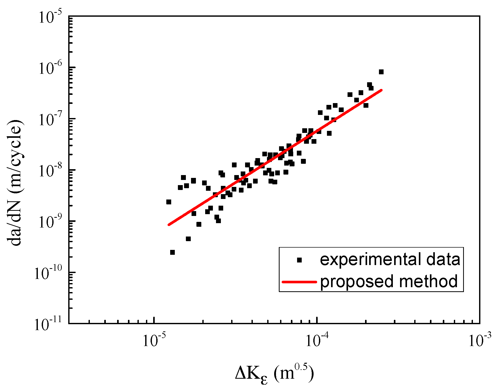
41]. The testing data are re-plotted in
Figure 4. The horizontal axis represents the strain intensity factor range and the vertical axis represents the crack growth rate. It can be seen clearly that all the testing data shrink into one line (and the dispersion is quite small). It is indicated that the strain intensity factor range could be a better driving force than the SIF range to depict the fatigue crack propagation behavior.
2.2. The Fatigue Life Prediction Model
A SIF-based equation proposed by Newman is employed, shown as Equation (5) [
42],
where
C1,
n1,
p1, and
q are fitting parameters and
g is related to the crack closure.
R is the stress ratio.
,
, and
are the threshold SIF, the maximum SIF, and the critical SIF, respectively. The fast growing stage has little impact on the fatigue life and so can be ignored. Moreover, in this investigation R is equal to −1 (the fully reversed loading), so the Equation (5) can be simplified as:
where
C2,
n2,
p2 are the fitting parameters. Next, the strain intensity factor replaces the SIF. The formula can be modified as:
where
C,
n, and
p are the fitting parameters and
is the threshold strain intensity factor. Thus, the fatigue life can be calculated by integrating the fatigue crack growth rate equation, which can be expressed as follows:
where
ai is the initial crack size and
ac is the critical crack size at failure. When the crack length is approaching
ac, the crack growth rate is very fast. Some previous studies claim that the fatigue life is not sensitive to the value of
ac [
5,
43] (in this study, it is determined by
Kc (
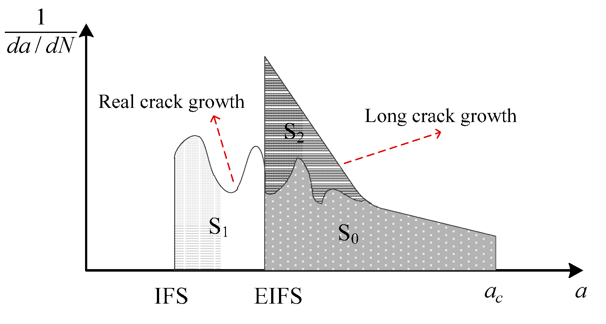
)). It can be observed from Equation (8) that the initial crack length plays an important role in the fatigue life evaluation. Since the real small crack growth is irregular and hard to describe accurately, the EIFS concept is proposed to estimate the small crack growth life [
5]. As shown in
Figure 5, the area S
1 and S
0 represent the fatigue life of the real crack, and the area S
2 and S
0 represent the life calculated by using EIFS. It is assumed that the area S
1 is equal to the area S
2. In other words, the long crack growth model and the EIFS are used to approximate the real small crack growth.
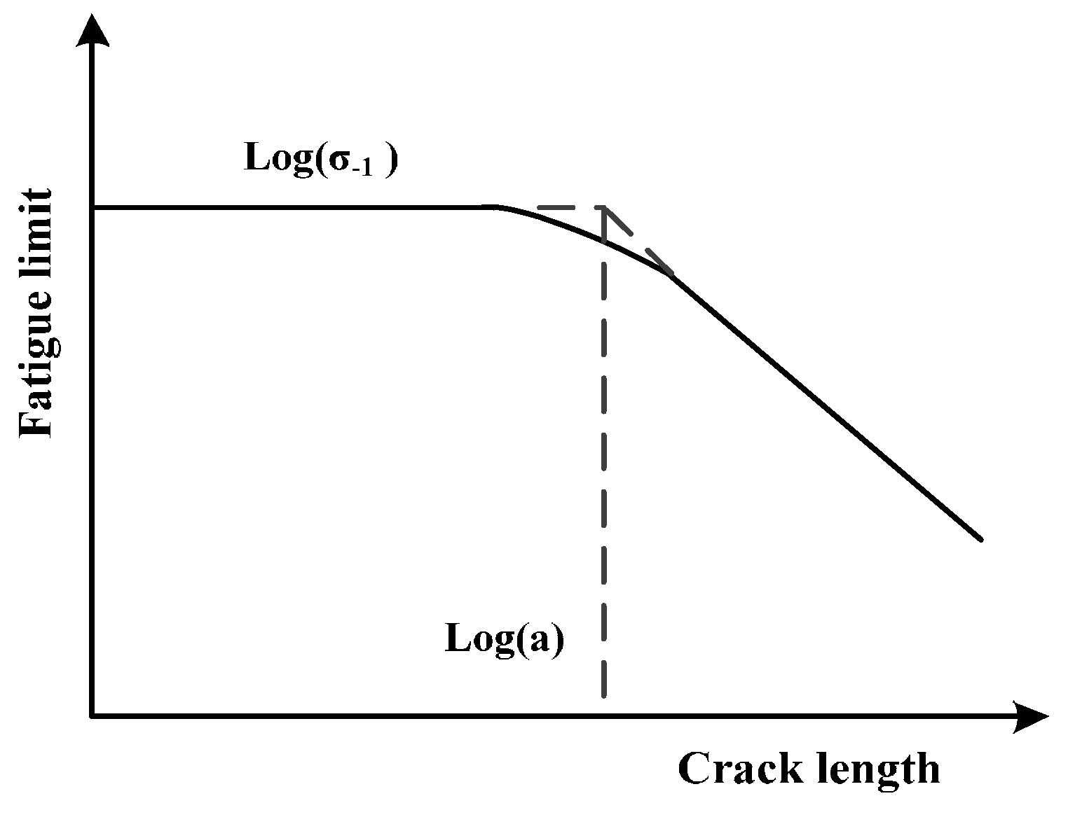
In
Figure 6, the Kitagawa-Takahashi diagram (KT diagram) shows the stress level decreases with the increase of the crack length until the stress reaches the fatigue limit [
44].
El Haddad [
45] et al. proposed an equation combining the threshold stress intensity factor range
and the fatigue limit
in which the crack length (a) is considered to be the EIFS. Under this condition, the stress and strain is almost linearly related, for the stress range is quite small. Thus, the EIFS can be calculated by the strain intensity factor and the value can be obtained by the threshold strain intensity factor and the fatigue limit strain:
where
is the fatigue limit strain. The threshold strain intensity factor and fatigue limit strain are defined as the threshold values, below which the fatigue life is infinite in theory.
Then, the EIFS is calculated by solving the Equation (10) numerically. Note that
γ is also the function of the crack length.
is determined by back-extrapolation (the detailed procedure can be found in Reference [
5]).
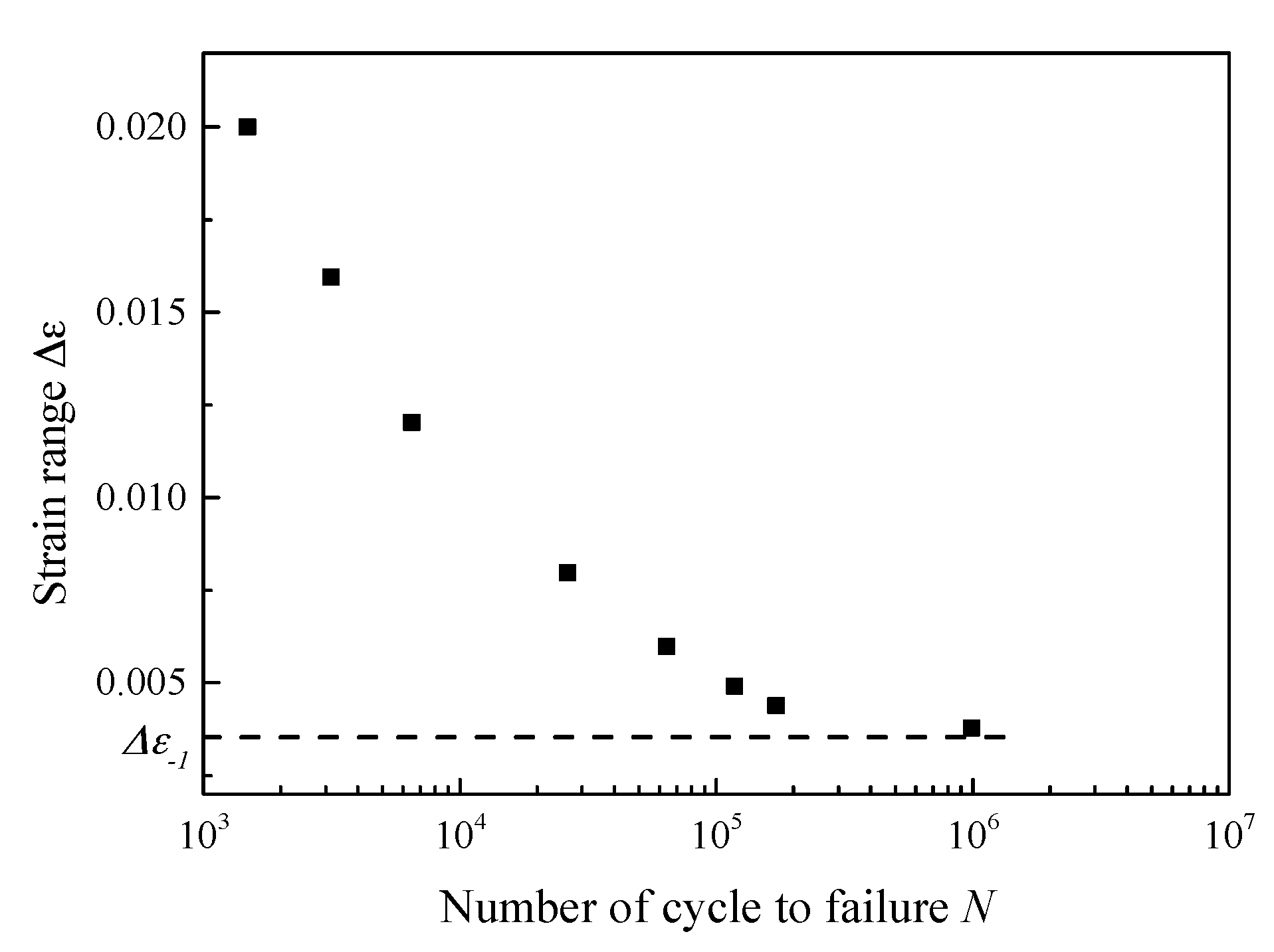
is obtained by analyzing the asymptotic properties of the
ε-N curve (as shown in
Figure 7). Then, the fatigue life can be estimated as:


