7.1. A Generalised Failure Time Distribution
One generalised linear model for ln(t
F) takes the form
where μ is a scaling parameter which in this application is given by
and σ is a shape parameter so that the random variable v can be interpreted as following a standardised distribution. v is obviously incorporated into the model to pick up the batch to batch variation present in the experimental data. As the nature of the creep failure time distribution is generally unknown, it makes sense to select the most general possible representation of this distribution. On such distribution is the generalised F distribution. Therefore, in this paper, the variable v is taken to be the logarithm of an F variate with 2κ
1 and 2κ
2 degrees of freedom. The probability density function (PDF) for v is then given by
where Γ() is the gamma function and μ and σ, together with κ
1 and κ
2, are the parameters of this four parameter log F distribution. Values of (κ
1, κ
2) equal to (1, 1), (1, ∞) and (∞, 1) correspond, respectively, to the logistic, extreme value for a minima and extreme value for a maxima for ln[t
F]. As κ
2 approaches infinity the distribution for v approaches the logarithm of a generalised gamma variate as presented by Stacy and Mihram [
10]. When σ = 1 the familiar gamma distribution is obtained. When (κ
1 = ∞, κ
2 = ∞) the distribution for ln[t
F] corresponds to a normal distribution (and so the variable v becomes the standard normal distribution). However, as specified in Equation (10), the distribution is degenerate in nature. Prentice [
11] has shown that such degeneracy can be avoided by transforming v in the following way
so that
The probability density function (PDF) for w can be found by substituting Equation (11) into Equation (10)
At κ
1 = κ
2 = ∞, w has a standard normal distribution. The probability density function (PDF) for y = ln[t
F] is
Values of (κ1, κ2) equal to (1, 1), (1, ∞), (∞, 1) and (∞, ∞) correspond, respectively, to the logistic, extreme value for a minima, extreme value for a maxima and normal distributions for ln[tF]. Consequently, values of (κ1, κ2) equal to (1, 1) and (∞, ∞) correspond, respectively, to the log-logistic and (non degenerate) log normal distribution for tF. The Weibull distribution for tF is obtained at (κ1, κ2) = (1, ∞). If in addition η = 1, the exponential distribution for tF is obtained. The generalised gamma distribution corresponds to κ2 = ∞ and this reduces to the gamma distribution for η = 1.
The distribution for ln[t
F] corresponding to κ
2 = ∞ is essentially the logarithm of a generalised gamma variate which has recently been applied by Evans [
12] to high temperature life time data. The PDF given by Equation (14) is positively skewed for κ
1 > κ
2, negatively skewed for κ
1 < κ
2 and symmetric for κ
1 = κ
2.
Within this framework, it is also easy to allow for the variability in failure times to depend on stress, which is a phenomenon often seen in large multi batch uniaxial creep test programs. One possible specification for this stress dependant heteroscedasticity that does not allow for a negative variance at any stress level is
so that β
1 = 0 corresponds to homoscedasticity or constant variability in failure times, which is the implicit assumption of the original Wilshire specification. The rth percentile time to failure is then given by
where w
k1,k2,r is the rth percentile of the logarithm of an F distributed variate with 2κ
1 and 2κ
2 degrees of freedom.
7.2. Parameter Estimation
The parameters μ, η, κ
1 and κ
2 can be estimated from a sample of observations on t
F. Suppose that a sample of n log (natural) times to failure have been collected. Assuming that these observations are independent, the probability of actually observing this sample of log times to failure is given by Equation (14) and the product rule of probability,
where L(μ, η, κ
1, κ
2) is called the likelihood of observing the sample of log times to failure, which of course depends on the values for μ, η, κ
1, κ
2. Within this framework, it makes sense to choose values for μ, η, κ
1 and κ
2 that maximise this likelihood. Because it is often easier to work with sums rather than products, values for μ, η, κ
1 and κ
2, are in practice chosen to maximise the log likelihood, ln L(μ, η, κ
1, κ
2).
The values for μ, η, κ1 and κ2 that maximise ln L(μ, η, κ1, κ2) are called maximum likelihood estimates and are given the symbols . Maximising the log of Equation (17) requires simultaneously solving the equations , ; , .
As Equation (17) stands, finding such a solution is rather difficult because these partial derivatives are not finite and in some cases are identically zero along the boundaries κ
1 = ∞ and κ
2 = ∞. This makes it all the more difficult to discriminate between various distributions for ln[t
F]—especially the log-normal distribution. As shown by Prentice [
11], the following re-parameterisation leads to a maximised log likelihood function with regular (finite and not identically zero) likelihood derivatives everywhere on the boundary κ
1 = ∞ and κ
2 = ∞
Under this parameterisation, the log-normal, Weibull, log-logistic, reciprocal Weibull, and generalised gamma distributions for t
F occur, respectively, at (q, p) values of (0, 0), (1, 0), (0, 1), (−1, 0) and (q > 0, 0). The maximum likelihood solution can be further simplified by using numerical rather than analytical derivatives and by treating q and p as fixed, so that maximisation of the log of Equation (9) only requires simultaneously solving the equations
As shown by Lawless [
13], this implies a simple two-step grid search procedure. For a given value of p and q and τ
*c and T
crit in Equations (9), (12), (17) and (18), first find the values
that maximise ln L(μ, η, q, p) by solving the above equations with the specified values for q, p and τ
*c, T
crit. Secondly, if this is done for various values of q, p, τ
*c and T
crit the largest of all these maximised log likelihood’s, termed the grand maximised log likelihood, can be obtained and so
, τ
*c and T
crit located. Berndt et al. [
14] give details of how these derivatives can be solved numerically.
7.3. Findings
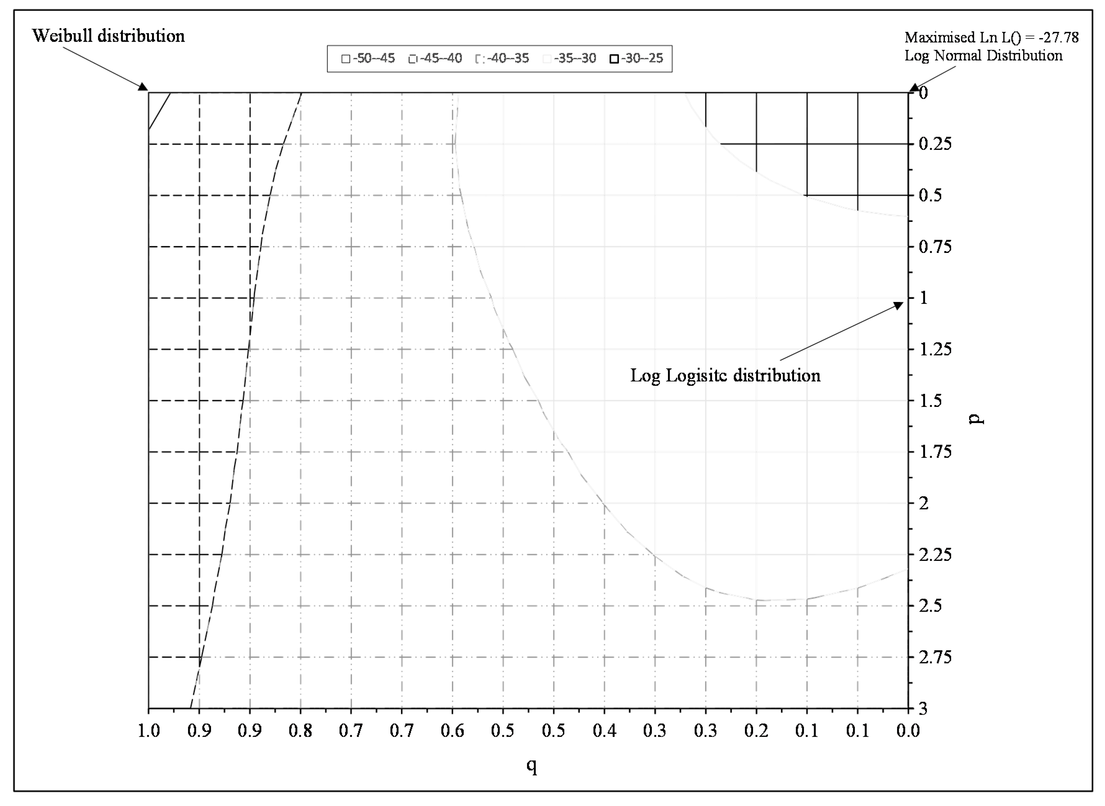
Figure 6 shows the results of the above grid search procedure and the ln of the likelihood function is maximised when p = q = 0, suggesting that the normal distribution for ln[t
F] best describes all the experimental failure times.
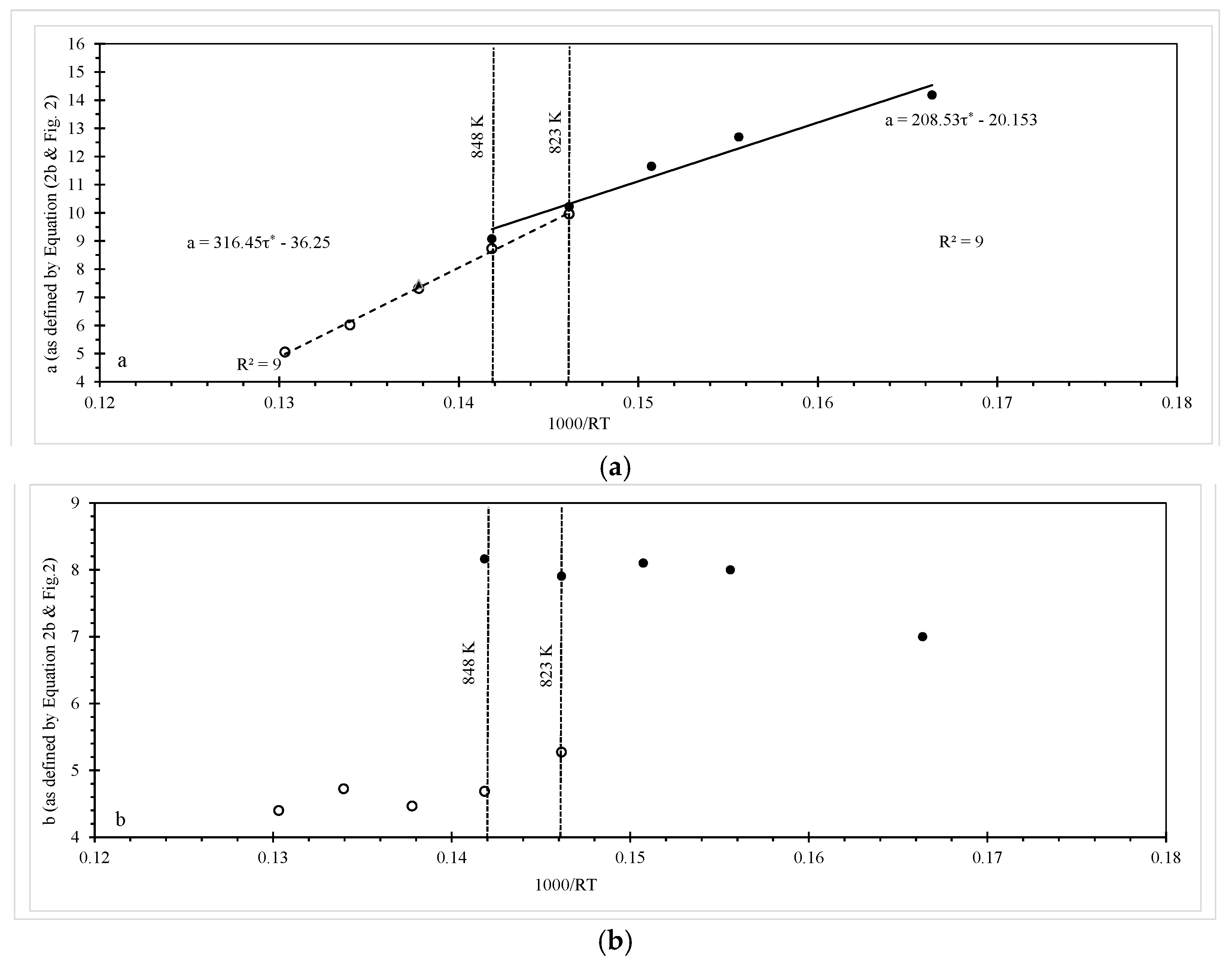
The maximum likelihood estimates for the unknown parameters in Equations (9), (15) and (18), associated with this grand maximised log likelihood, are shown in
Table 2. The parameter estimates in
Table 2 are similar to those in
Table 1 and do not alter the interpretations made earlier about creep mechanisms. However, the statistical significance of β
1 means that the variability in the experimental times to failure increases with increasing stress levels. This is clearly seen in
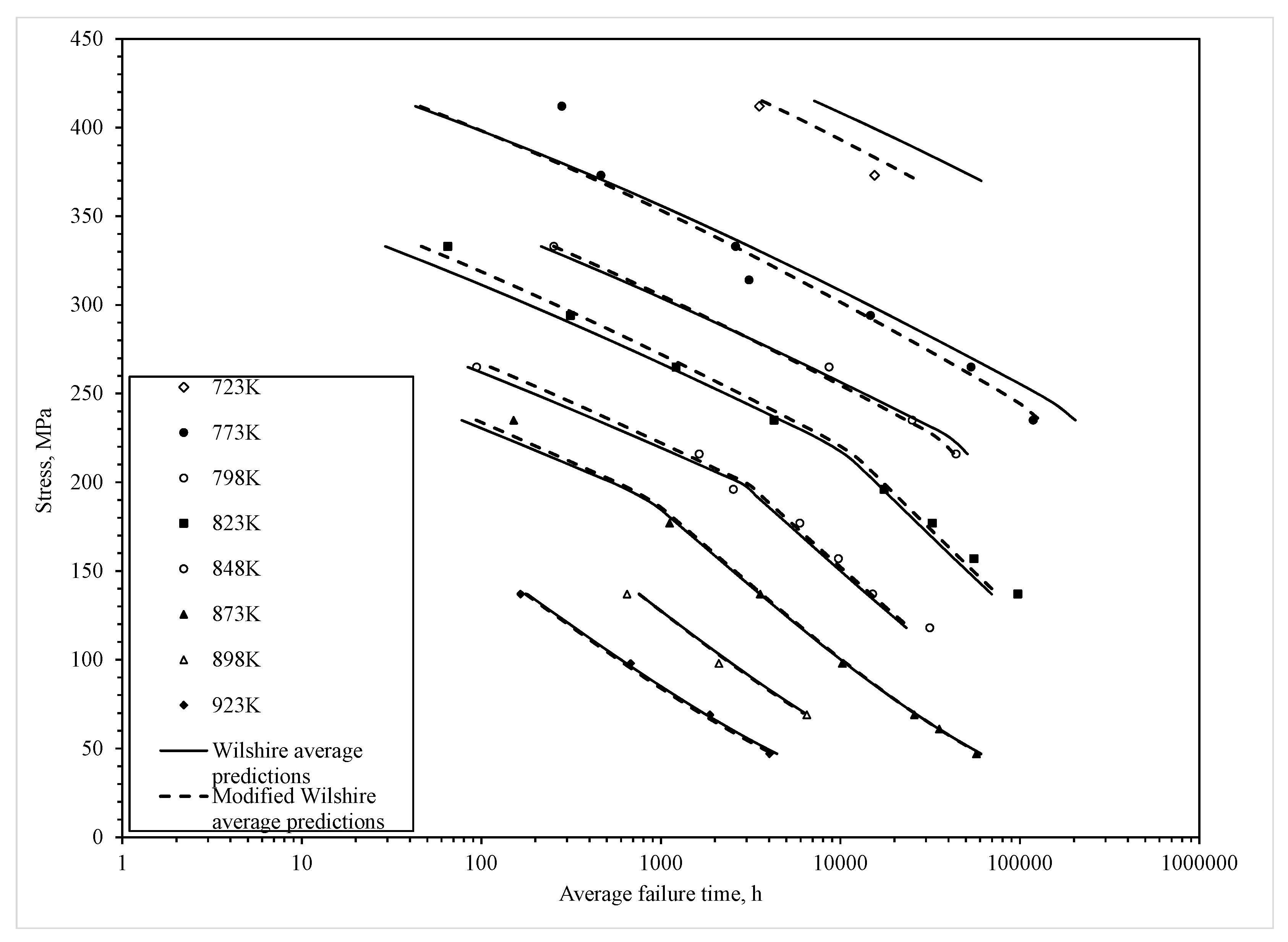
Figure 7, where the r = 0.05 and r = 0.995 percentiles of the time to failure are shown and are based on Equation (16). This produced a 99% prediction band for times to failure around the median (r = 0.5 percentile) time to failure shown as the solid segmented line in
Figure 7. In this figure, the left most plot of data are the results from applying the traditional Wilshire equation, based on the parameters in
Table 1, with a constant failure time variance and a normal distribution. The constant variance is seen by the constant width of the prediction bands. At the higher stress levels, this specification does not work well with more data points falling outside this band compared to at the lower stress levels. That is, the bands are too wide at lower stresses and to narrow at the higher stresses.
The plot of data to the right is the modified Wilshire equation based on the parameters in
Table 2 that allows for non-constant variance within the normal distribution. It can now be seen that very few data points are outside this prediction band, and the narrower width of the band at the lower stresses allows for less conservative safe life estimates to be made for this material, whilst still maintaining a less than 0.05% chance of failure before this safe life prediction.
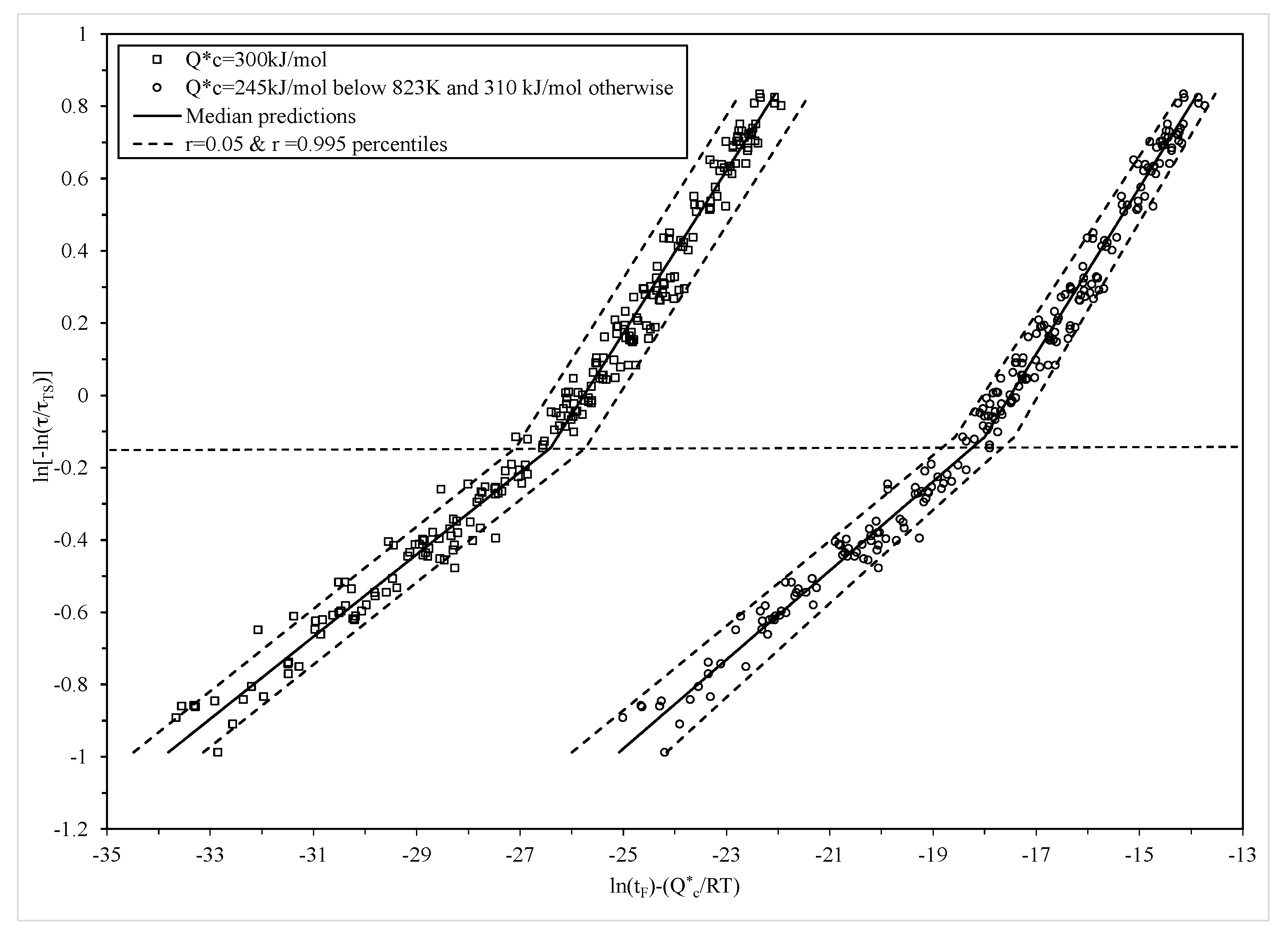
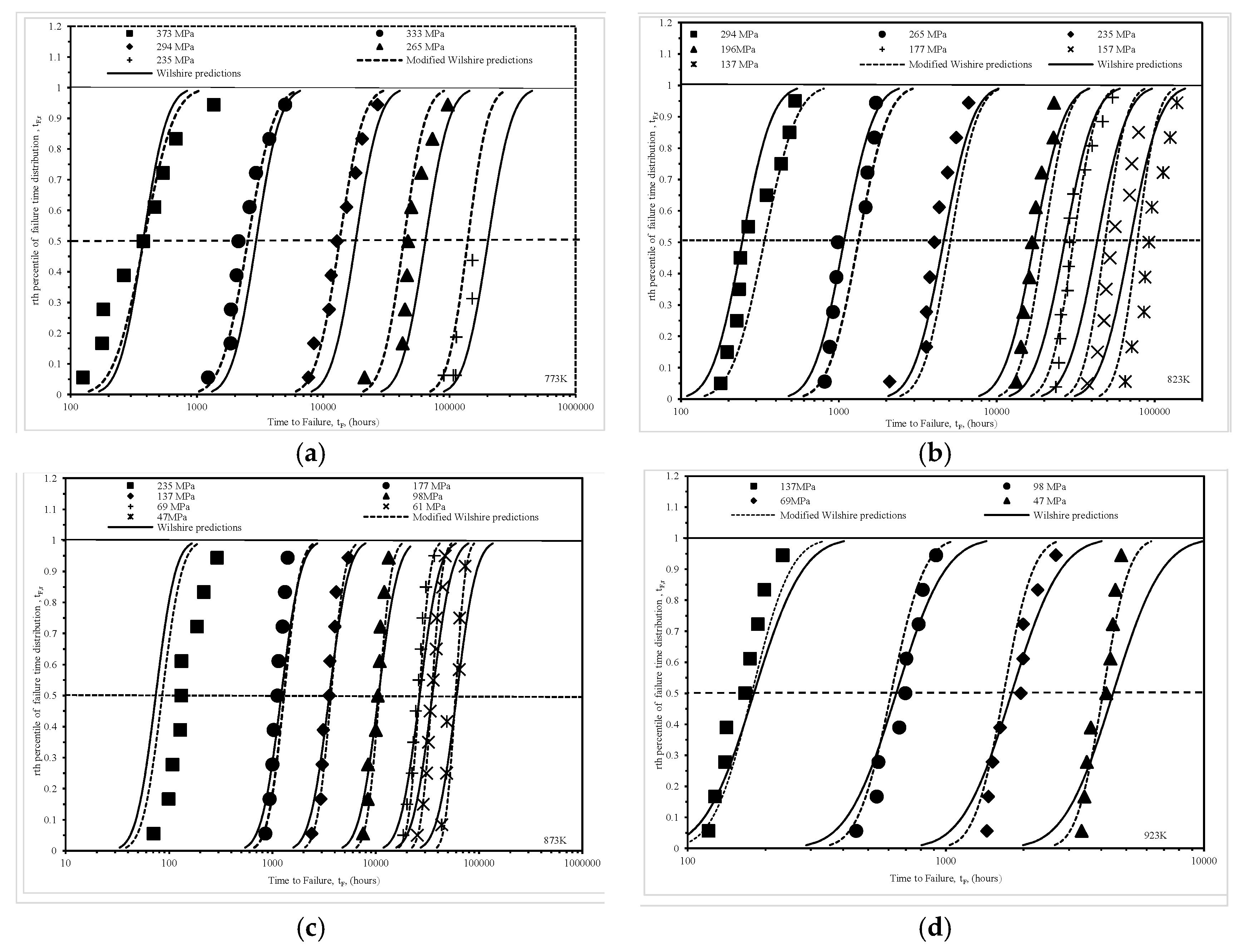
Figure 8 presents another way of comparing how well these two approaches do at predicting various percentiles of the time to failure distribution. In this figure the shown data points are the empirical percentiles as they are calculated only from the failure times themselves using
and as such make no distributional assumptions in their derivation. In Equation (20), n represents the number of failed specimens obtained at a particular stress–temperature combination and i is a rank index—equal to 1 for the smallest recorded failure time through to n for the largest recorded failure time at this test condition.
In
Figure 8, these empirical percentiles are plotted against the actual failure times at various stress–temperature combination to yield the symbol data points shown. The curves then show the rth percentile failure predictions obtained using the traditional Wilshire and modified Wilshire approaches. Highlighted with a horizontal line is the median actual and predicted time to failure at each of the stress–temperature combinations. At 773 K, it is clear that the modified approach yields better median time to failure predictions at all the different stress levels and, whilst still not perfect, it also yields better predictions at the tail ends of the failure time distribution as well.
The same picture emerges at 873 K, although both techniques fail to predict any percentile time to failure at the highest stress of 235 MPa. At 923 K, the modified approach clearly predicts the shape of the actual failure time distribution much better than the traditional Wilshire approach, but at the highest stress neither approach has worked particularly well—even though the median predicted time to failure is reasonable. Finally, at 823 K although neither approach describes the failure time distribution well at the very lowest stresses, the modified approach is the better of the two.


