
Characterizing Hypervelocity Impact (HVI)-Induced Pitting Damage Using Active Guided Ultrasonic Waves: From Linear to Nonlinear


 and
and 
Abstract
:1. Introduction
2. Theory and Rationale: Nonlinear Guided Waves
3. Numerical Simulation of Nonlinear Guided Waves
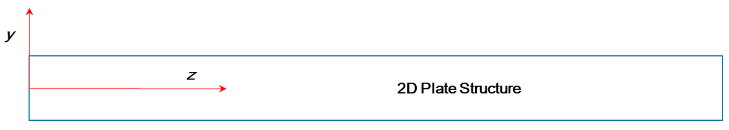
3.1. 2-D Scenario
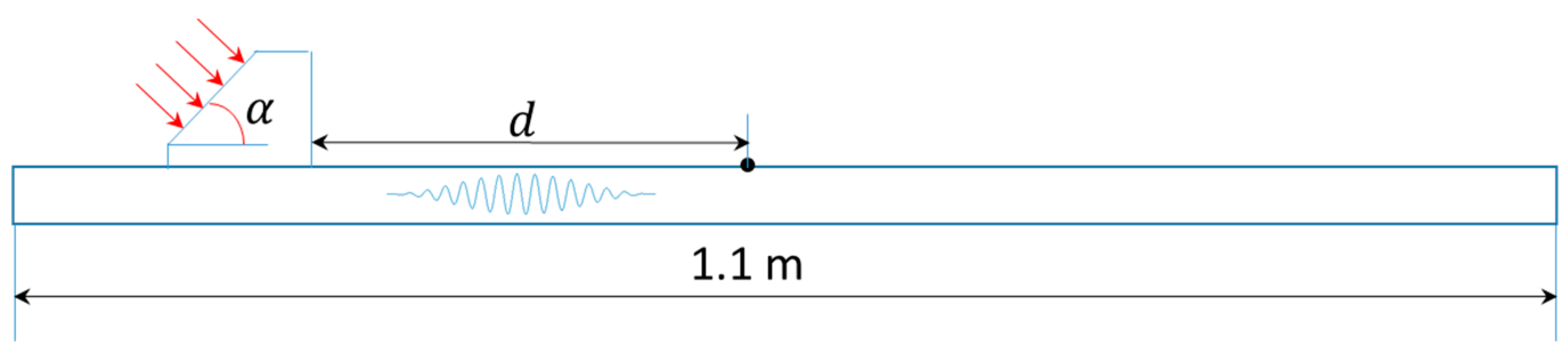
3.1.1. Problem Description
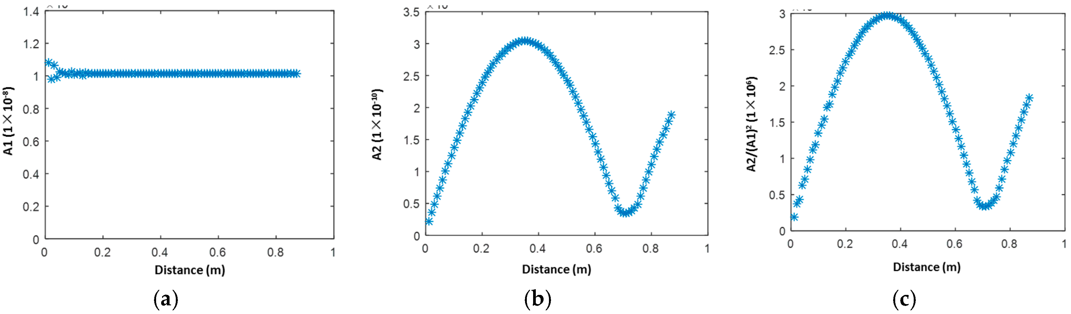
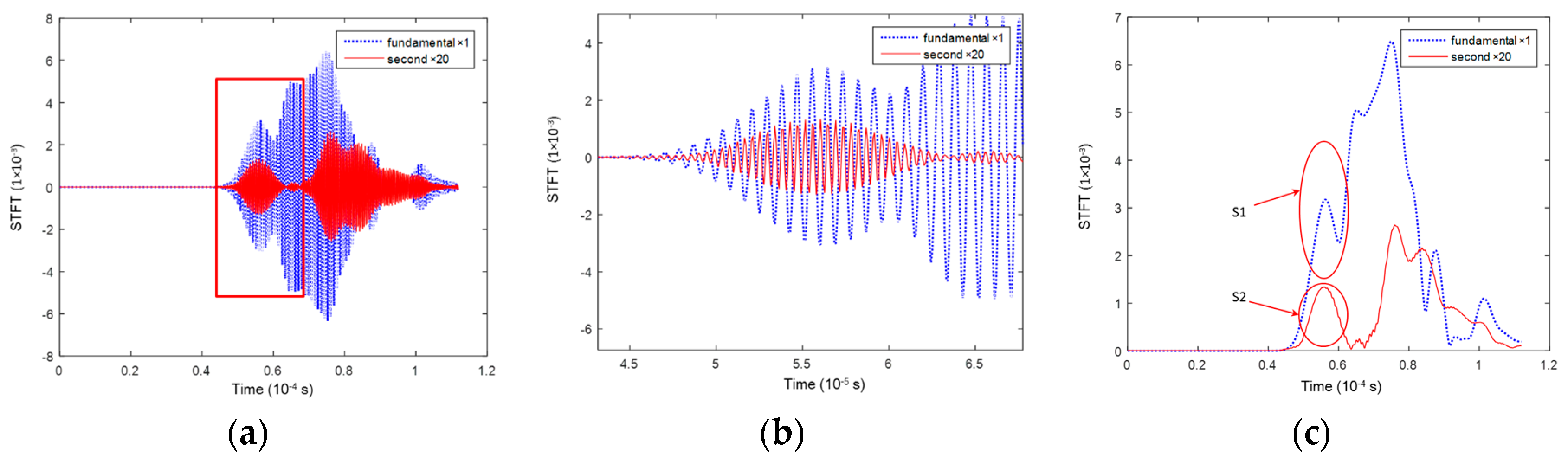
3.1.2. Results and Discussion
3.2. 3-D Scenario
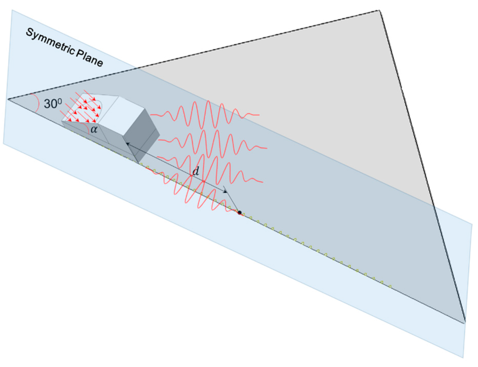
3.2.1. Problem Description
3.2.2. Results and Discussion
4. Experimental Validation
4.1. HVI Experiment
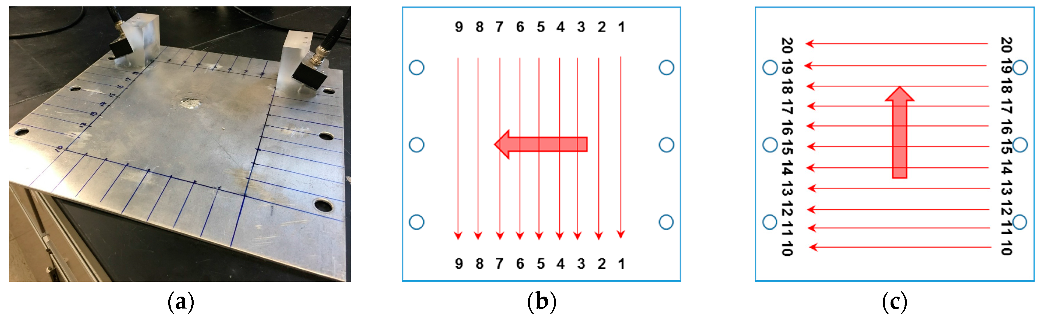
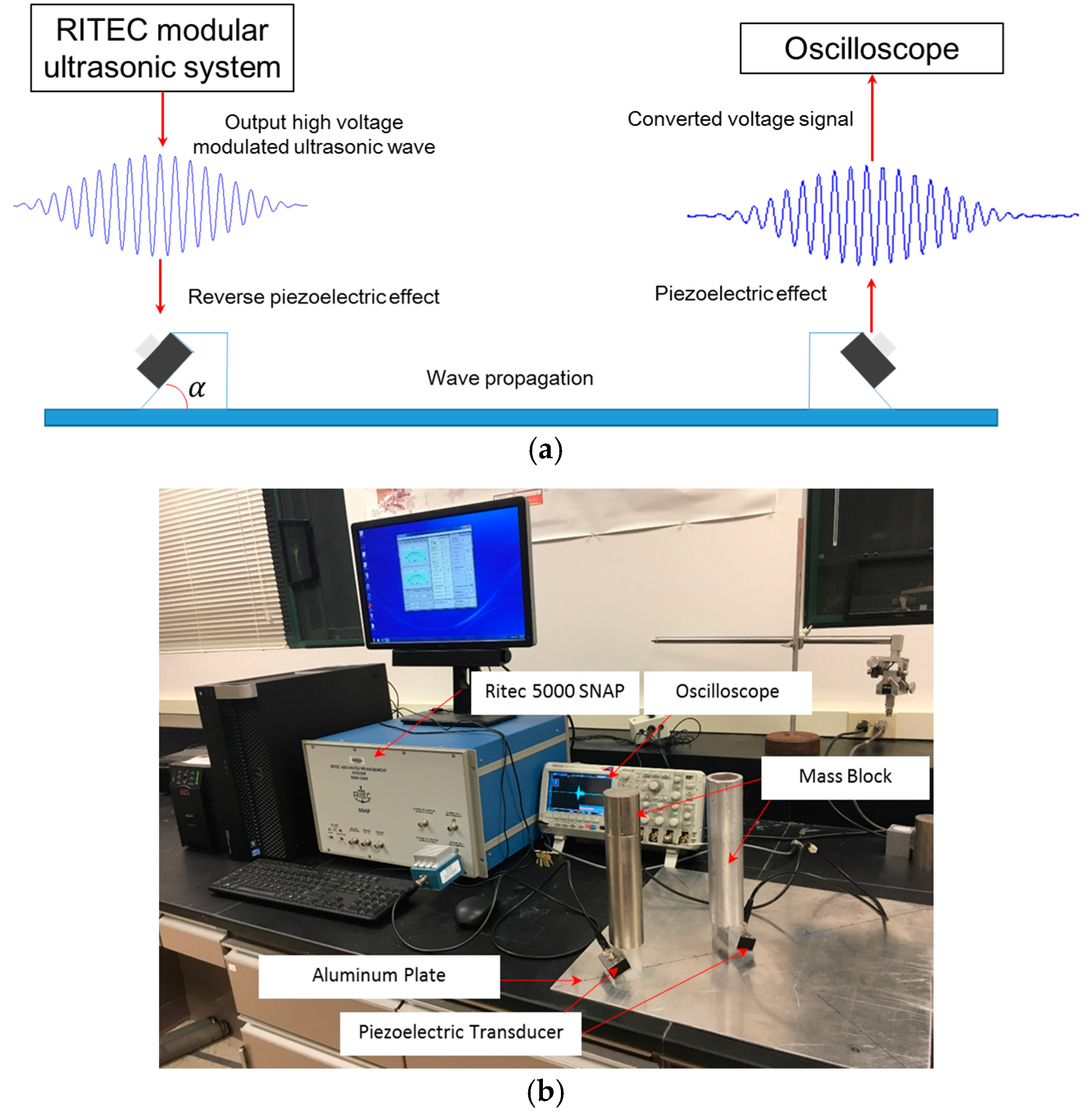
4.1.1. Experimental Setups
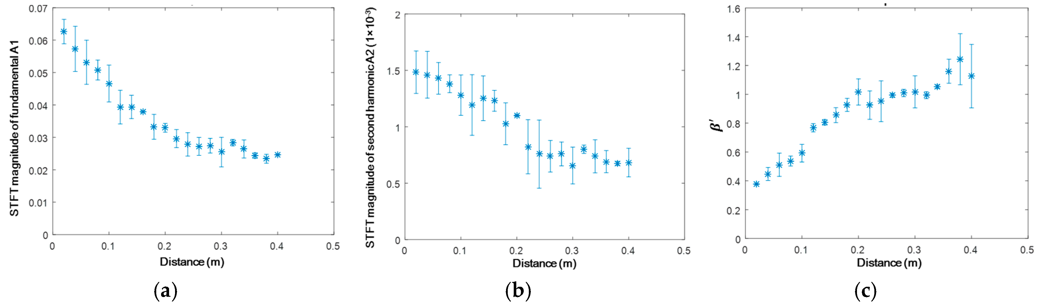
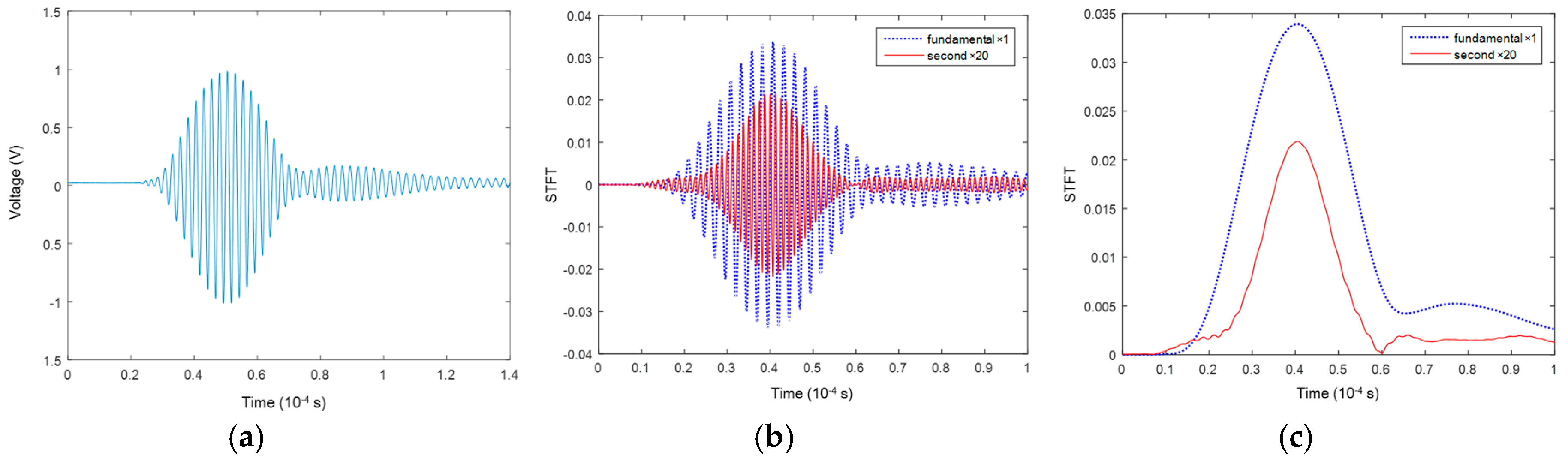
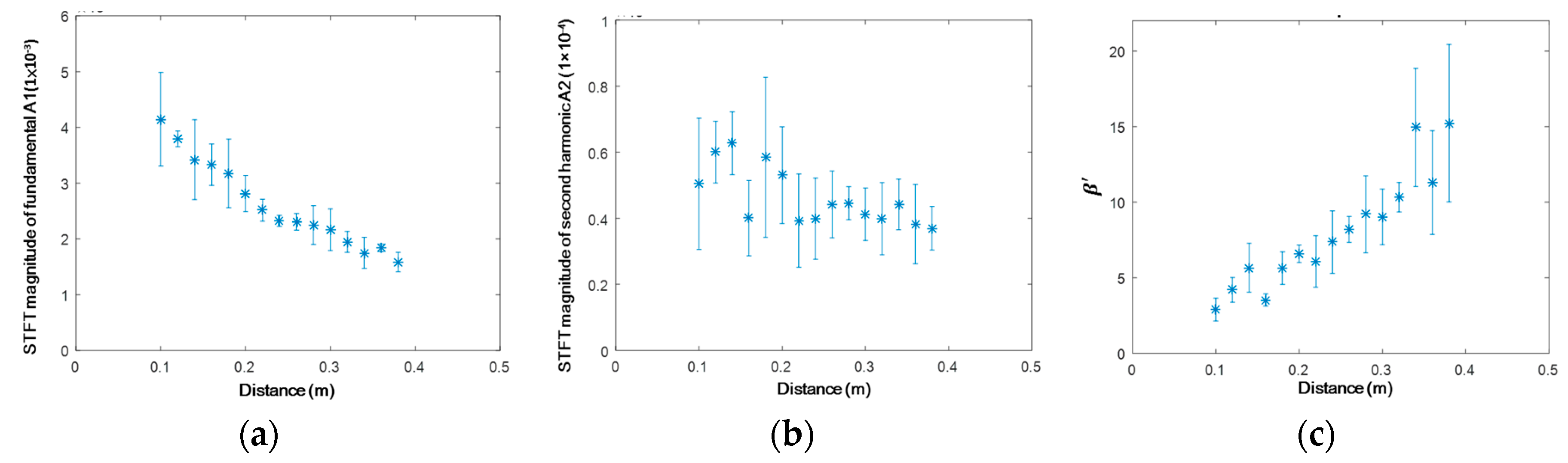
4.1.2. Results and Discussion
4.2. Development of Linear/Nonlinear Damage Indices
5. Damage Characterization of HVI-Induced Pitting Damage Using Damage Indices
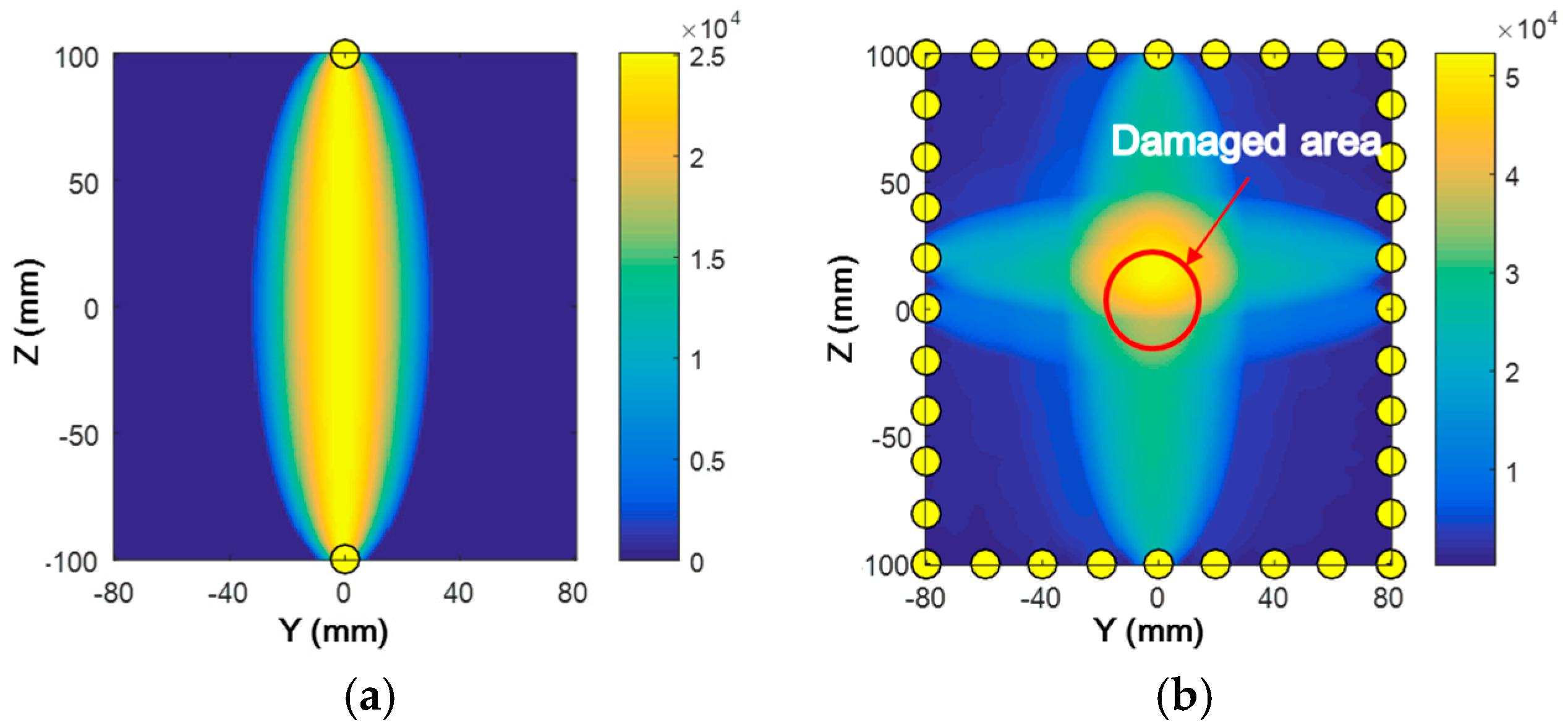
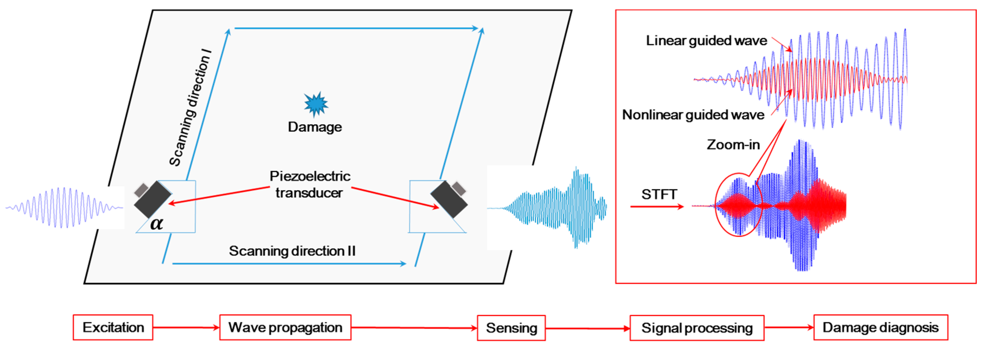
5.1. Construction of Probabilistic Imaging Using the Damage Index
5.2. Imaging: Results and Discussion
6. Conclusions
Acknowledgments
Author Contributions
Conflicts of Interest
References
- IADC W G. Members. Sensor Systems to Detect Impacts on Spacecraft IADC-08-03; IADC: Houston, TX, USA, 2013. [Google Scholar]
- Christiansen, E.; Hyde, J.; Bernhard, R. Space shuttle debris and meteoroid impacts. Adv. Space Res. 2004, 34, 1097–1103. [Google Scholar] [CrossRef]
- Drolshagen, G. Impact effects from small size meteoroids and space debris. Adv. Space Res. 2008, 41, 1123–1131. [Google Scholar] [CrossRef]
- NASA. Space Debris and Human Spacecraft. Available online: http://www.nasa.gov/mission_pages/station/news/orbital_debris.html (accessed on 13 May 2017).
- NASA Orbital Debris Program Office. Monthly number of objects in earth orbit by object type. Orbital Debris Q. News 2016, 20, 13. [Google Scholar]
- European Space Agency. Impact Chip. Available online: http://www.esa.int/spaceinimages/Images/2016/05/Impact_chip (accessed on 13 May 2017).
- Taylor, E.A.; Herbert, M.K.; Vaughan, B.A.M.; McDonnell, J.A.M. Hypervelocity impact on carbon fibre reinforced plastic/aluminium honeycomb: Comparison with whipple bumper shields. Int. J. Impact Eng. 1999, 23, 883–893. [Google Scholar] [CrossRef]
- Su, Z.; Ye, L.; Lu, Y. Guided lamb waves for identification of damage in composite structures: A review. J. Sound Vib. 2006, 295, 753–780. [Google Scholar] [CrossRef]
- Qiu, L.; Yuan, S.F.; Zhang, X.Y.; Wang, Y. A time reversal focusing based impact imaging method and its evaluation on complex composite structures. Smart Mater. Struct. 2011, 20, 105014. [Google Scholar] [CrossRef]
- Yuan, S.; Ren, Y.; Qiu, L.; Mei, H. A multi-response-based wireless impact monitoring network for aircraft composite structures. IEEE Trans. Ind. Electron. 2016, 63, 7712–7722. [Google Scholar] [CrossRef]
- Qiu, L.; Yuan, S.; Liu, P.; Qian, W. Design of an all-digital impact monitoring system for large-scale composite structures. IEEE Trans. Instrum. Meas. 2013, 62, 1990–2002. [Google Scholar] [CrossRef]
- Giurgiutiu, V. Tuned lamb wave excitation and detection with piezoelectric wafer active sensors for structural health monitoring. J. Intell. Mater. Syst. Struct. 2005, 16, 291–305. [Google Scholar] [CrossRef]
- Li, F.; Su, Z.; Ye, L.; Meng, G. A correlation filtering-based matching pursuit (cf-mp) for damage identification using lamb waves. Smart Mater. Struct. 2006, 15, 1585–1594. [Google Scholar] [CrossRef]
- Zhou, C.; Su, Z.; Cheng, L. Quantitative evaluation of orientation-specific damage using elastic waves and probability-based diagnostic imaging. Mech. Syst. Signal Process. 2011, 25, 2135–2156. [Google Scholar] [CrossRef]
- Alleyne, D.N.; Cawley, P. The interaction of lamb waves with defects. IEEE Trans. Ultrason. Ferroelectr. 1992, 39, 381–397. [Google Scholar] [CrossRef] [PubMed]
- Jhang, K.-Y. Nonlinear ultrasonic techniques for nondestructive assessment of micro damage in material: A review. Int. J. Precis. Eng. Manuf. 2009, 10, 123–135. [Google Scholar] [CrossRef]
- Su, Z.; Zhou, C.; Hong, M.; Cheng, L.; Wang, Q.; Qing, X. Acousto-ultrasonics-based fatigue damage characterization: Linear versus nonlinear signal features. Mech. Syst. Signal Process. 2014, 45, 225–239. [Google Scholar] [CrossRef]
- Hong, M.; Su, Z.; Lu, Y.; Sohn, H.; Qing, X. Locating fatigue damage using temporal signal features of nonlinear lamb waves. Mech. Syst. Signal Process. 2015, 60, 182–197. [Google Scholar] [CrossRef]
- Deng, M. Cumulative second-harmonic generation of lamb-mode propagation in a solid plate. J. Appl. Phys. 1999, 85, 3051–3058. [Google Scholar] [CrossRef]
- Deng, M. Cumulative second-harmonic generation accompanying nonlinear shear horizontal mode propagation in a solid plate. J. Appl. Phys. 1998, 84, 3500–3505. [Google Scholar]
- De Lima, W.J.N.; Hamilton, M.F. Finite-amplitude waves in isotropic elastic plates. J. Sound Vib. 2003, 265, 819–839. [Google Scholar] [CrossRef]
- Lissenden, C.J.; Liu, Y.; Choi, G.W.; Yao, X. Effect of localized microstructure evolution on higher harmonic generation of guided waves. J. Nondestruct. Eval. 2014, 33, 178–186. [Google Scholar] [CrossRef]
- Liu, Y.; Chillara, V.K.; Lissenden, C.J.; Rose, J.L. Third harmonic shear horizontal and rayleigh lamb waves in weakly nonlinear plates. J. Appl. Phys. 2013, 114, 114908. [Google Scholar] [CrossRef]
- Chillara, V.K.; Lissenden, C.J. Interaction of guided wave modes in isotropic weakly nonlinear elastic plates: Higher harmonic generation. J. Appl. Phys. 2012, 111, 124909. [Google Scholar] [CrossRef]
- Chillara, V.K.; Lissenden, C.J. Nonlinear guided waves in plates: A numerical perspective. Ultrasonics 2014, 54, 1553–1558. [Google Scholar] [CrossRef] [PubMed]
- Norris, A.N. Finite-amplitude waves in solids. In Nonlinear Acoustics; Hamilton, M.F., Ed.; Academic Press: San Diego, CA, USA, 1998; pp. 263–277. [Google Scholar]
- Landau, L.; Lifshitz, E. Theory of Elasticity, 3rd ed.; Pergamon Press: Oxford, UK, 1986. [Google Scholar]
- Thomas, J.F., Jr. Third-order elastic constants of aluminum. Phys. Rev. 1968, 175, 955–962. [Google Scholar] [CrossRef]
- Auld, B.A. Acoustic Fields and Waves in Solids; Wiley: New York, NY, USA, 1973. [Google Scholar]
- Rose, J.L. Ultrasonic Guided Waves in Solid Media; Cambridge University Press: Cambridge, UK, 2014. [Google Scholar]
- Chillara, V.K.; Lissenden, C.J. Review of nonlinear ultrasonic guided wave nondestructive evaluation: Theory, numerics, and experiments. Opt. Eng. 2016, 55, 011002. [Google Scholar] [CrossRef]
- Hong, M.; Su, Z.; Wang, Q.; Cheng, L.; Qing, X. Modeling nonlinearities of ultrasonic waves for fatigue damage characterization: Theory, simulation, and experimental validation. Ultrasonics 2014, 54, 770–778. [Google Scholar] [CrossRef] [PubMed]
- Liu, Y.; Chillara, V.K.; Lissenden, C.J. On selection of primary modes for generation of strong internally resonant second harmonics in plate. J. Sound Vib. 2013, 332, 4517–4528. [Google Scholar] [CrossRef]
- Torello, D.; Thiele, S.; Matlack, K.H.; Kim, J.-Y.; Qu, J.; Jacobs, L.J. Diffraction, attenuation, and source corrections for nonlinear rayleigh wave ultrasonic measurements. Ultrasonics 2015, 56, 417–426. [Google Scholar] [CrossRef] [PubMed]
- Matlack, K.H.; Kim, J.-Y.; Jacobs, L.J.; Qu, J. Experimental characterization of efficient second harmonic generation of lamb wave modes in a nonlinear elastic isotropic plate. J. Appl. Phys. 2011, 109, 014905. [Google Scholar] [CrossRef]
- Zuo, P.; Zhou, Y.; Fan, Z. Numerical and experimental investigation of nonlinear ultrasonic lamb waves at low frequency. Appl. Phys. Lett. 2016, 109, 021902. [Google Scholar] [CrossRef]
- Bermes, C.; Kim, J.-Y.; Qu, J.; Jacobs, L.J. Experimental characterization of material nonlinearity using lamb waves. Appl. Phys. Lett. 2007, 90, 021901. [Google Scholar] [CrossRef]
- Zhao, X.L.; Gao, H.D.; Zhang, G.F.; Ayhan, B.; Yan, F.; Kwan, C.; Rose, J.L. Active health monitoring of an aircraft wing with embedded piezoelectric sensor/actuator network: I. Defect detection, localization and growth monitoring. Smart Mater. Struct. 2007, 16, 1208–1217. [Google Scholar] [CrossRef]


| Part | Elastic Modulus (GPa) | Poisson’s Ratio | Density (kg/m3) |
|---|---|---|---|
| Plexiglas wedge | 4.12 | 0.39 | 1180 |
| Aluminum plate | 68.9 | 0.33 | 2780 |
| A (GPa) | B (GPa) | C (GPa) | |
| −320 | −200 | −190 |
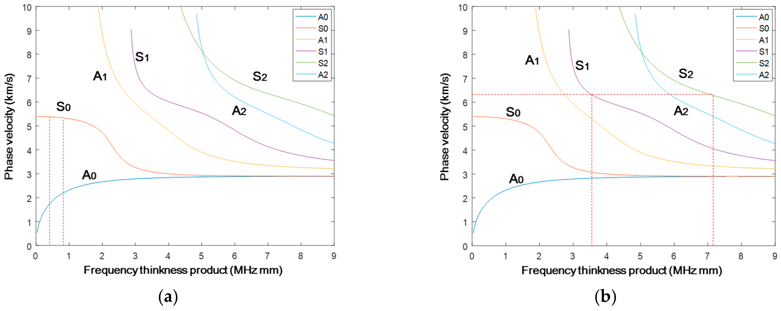
| Case No. | Plate Thickness (mm) | Excitation Frequency (kHz) | Frequency Thickness Product (MHz mm) | Mode Pair | Phase Velocity (m/s) |
|---|---|---|---|---|---|
| 1 | 1 | 400 | 0.4–0.8 | S0-S0 | 5261–5221 |
| 2 | 3 | 1178 | 3.534–7.068 | S1-S2 | 6241–6241 |
© 2017 by the authors. Licensee MDPI, Basel, Switzerland. This article is an open access article distributed under the terms and conditions of the Creative Commons Attribution (CC BY) license (http://creativecommons.org/licenses/by/4.0/).
Share and Cite
Liu, M.; Wang, K.; Lissenden, C.J.; Wang, Q.; Zhang, Q.; Long, R.; Su, Z.; Cui, F. Characterizing Hypervelocity Impact (HVI)-Induced Pitting Damage Using Active Guided Ultrasonic Waves: From Linear to Nonlinear. Materials 2017, 10, 547. https://doi.org/10.3390/ma10050547
Liu M, Wang K, Lissenden CJ, Wang Q, Zhang Q, Long R, Su Z, Cui F. Characterizing Hypervelocity Impact (HVI)-Induced Pitting Damage Using Active Guided Ultrasonic Waves: From Linear to Nonlinear. Materials. 2017; 10(5):547. https://doi.org/10.3390/ma10050547
Chicago/Turabian StyleLiu, Menglong, Kai Wang, Cliff J. Lissenden, Qiang Wang, Qingming Zhang, Renrong Long, Zhongqing Su, and Fangsen Cui. 2017. "Characterizing Hypervelocity Impact (HVI)-Induced Pitting Damage Using Active Guided Ultrasonic Waves: From Linear to Nonlinear" Materials 10, no. 5: 547. https://doi.org/10.3390/ma10050547
APA StyleLiu, M., Wang, K., Lissenden, C. J., Wang, Q., Zhang, Q., Long, R., Su, Z., & Cui, F. (2017). Characterizing Hypervelocity Impact (HVI)-Induced Pitting Damage Using Active Guided Ultrasonic Waves: From Linear to Nonlinear. Materials, 10(5), 547. https://doi.org/10.3390/ma10050547