
Interacting Effects Induced by Two Neighboring Pits Considering Relative Position Parameters and Pit Depth

School of Aerospace Engineering, Xiamen University, Xiamen 361005, Fujian, China
*
Authors to whom correspondence should be addressed.
Materials 2017, 10(4), 398; https://doi.org/10.3390/ma10040398
Submission received: 30 January 2017
/
Revised: 26 March 2017
/
Accepted: 7 April 2017
/
Published: 9 April 2017
(This article belongs to the Special Issue Stress Corrosion Cracking in Materials)
Abstract
:For pre-corroded aluminum alloy 7075-T6, the interacting effects of two neighboring pits on the stress concentration are comprehensively analyzed by considering various relative position parameters (inclination angle θ and dimensionless spacing parameter λ) and pit depth (d) with the finite element method. According to the severity of the stress concentration, the critical corrosion regions, bearing high susceptibility to fatigue damage, are determined for intersecting and adjacent pits, respectively. A straightforward approach is accordingly proposed to conservatively estimate the combined stress concentration factor induced by two neighboring pits, and a concrete application example is presented. It is found that for intersecting pits, the normalized stress concentration factor Ktnor increases with the increase of θ and λ and always reaches its maximum at θ = 90°, yet for adjacent pits, Ktnor decreases with the increase of λ and the maximum value appears at a slight asymmetric location. The simulations reveal that Ktnor follows a linear and an exponential relationship with the dimensionless depth parameter Rd for intersecting and adjacent cases, respectively.
1. Introduction
Pitting corrosion is considered to be one of the most significant degradation mechanisms as it causes stress concentration and facilitates crack initiation, thus accelerating structural failure under fatigue loading conditions [1,2,3]. Therefore, understanding the stress environment around corrosion pits can assist the early prediction of critical regions bearing a relatively high probability of crack initiation, which is of particular significance to maintain structural integrity, especially for aircrafts, offshore structures, and other applications with high criticality or low tolerance of unwanted degradation.
It is believed that pit size, location, geometry, and the interaction with other pits are dominant factors which affect the stress concentration. A number of studies have been conducted to discuss the influence of the first three factors [4,5,6,7,8,9,10], yet limited research has focused on the interacting effects induced by neighboring pits. Domínguez et al. [11] examined the stress concentration for two close pitting holes located on the hourglass-shape specimen of aluminum alloy 6061-T6, and found that the stress concentration factor (SCF) increased exponentially with the proximity of pitting holes under the rotating-bending loading condition. Han et al. [12] studied the mechanical property of transmission pipelines with inner corrosion defects via the finite element method. Results showed that for the pipeline with two or three longitudinally-aligned corrosion defects, high stress areas and the plastic strain increased rapidly along the axial direction with the increasing of the inner pressure. By conducting 2D simulations, Kolios et al. [13] revealed that a lower spacing between pits resulted in a higher SCF, and colluded pits had a smaller stress-concentrating effect than pits spaced at a larger distance from each other. Hou et al. [14] discussed the stress concentration induced by two adjacent pits under a uniaxial tension loading condition. They pointed out that the SCF decreased nonlinearly with the increasing of the spacing between two transverse pits, and the interaction between two longitudinal pits should be ignored in the SCF calculation. Pidaparti et al. [15] predicted the stress distribution on a corroded random surface and found that the single pit induced a stress about 70% higher than the two-pit case for a 74-day corroded specimen. Xu [16] investigated the tensile behavior of eight different-depth spherical pits equally distributed at four lines along the axial direction on the reinforcement surface, and emphasized that the most disadvantageous location coincided with the deepest pit. The above-mentioned studies, however, mainly focus on neighboring pits aligned along transverse and/or longitudinal directions, which is obviously insufficient when comparing to the random spatial distribution of pitting corrosion in the actual environment. Furthermore, the influence of the pit depth on interacting effects has scarcely been taken into account in the available publications.
In our previous works [17,18], high-cycle fatigue tests were conducted for the pre-corroded aluminum alloy (AA) 7075-T6 specimens. Fracture analysis showed that under 120 h and 240 h pre-corrosion conditions, 64.9% (24 out of 37 pieces) and 44.1% (15 out of 34 pieces) of the specimens respectively failed due to the propagation of fatigue cracks originating at two neighboring pits. This is considered to be an interesting phenomenon and deserved further investigation.
In this work, for pre-corroded AA7075-T6 specimens, numerical simulations are carried out to investigate how a neighboring pit will exert influence on the stress field caused by a single pit, and how the critical corrosion region is identified for two intersecting and adjacent pits, respectively. By synthetically considering the pit depth and the relative position parameters, a straightforward approach is proposed to conservatively estimate the combined stress concentration factor (C-SCF) induced by two neighboring pits.
2. Finite Element Model
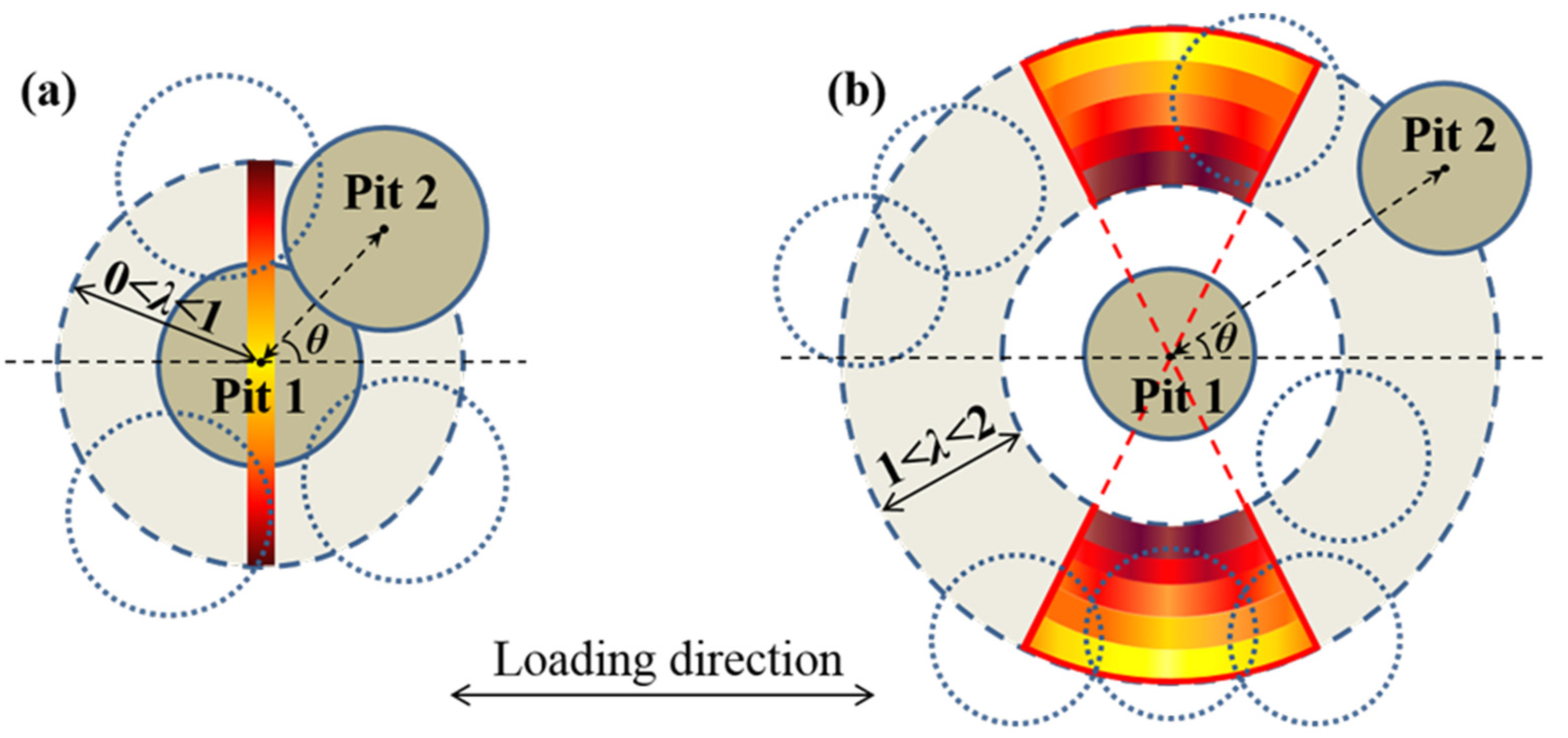
Details of the model for two neighboring pits are illustrated in Figure 1. The geometry involves a cuboid (10 mm × 6 mm × 2 mm) containing Pit 1 and Pit 2 on its top surface. The actual pit is idealized with a hemi-elliptical shape and is assumed to be capable of representing the stress field around the actual pit [19]. In order to examine the effect of the spatial distribution on the C-SCF, Pit 1 is placed at the center of the gage area as a reference for comparison, while Pit 2 is located at a random location on the top surface. Thus, the arrangements of Pit 1 and Pit 2, according to their relative positions, can be classified into two cases: adjacent pits and intersecting pits, as exemplified in Figure 1a.
Two relative position parameters, θ and λ, are introduced to quantitatively describe the relative locations of Pit 1 and Pit 2, which is illustrated in Figure 1b by taking two adjacent pits as an example. Here, θ is defined as the inclination angle between the loading direction and the line connecting centers of the two pits, and λ as a dimensionless parameter is used to measure the proximity of the two pits and is defined below,
where D is the spacing between the centers of Pit 1 and Pit 2, and r the radius for both pits, which is assigned to be 50 μm in our study. To clarify the influence of the pit depth (d) on interacting effects, we configure the depth of Pit 1 (d1) with three settings: 30 μm, 50 μm, and 100 μm, respectively, which correspondingly represent shallow, hemi-spherical, and deep pits. For Pit 2, we consider two cases of the pit depth (d2), which is either shallower than (d2 < d1) or identical with (d2 = d1 = d) that of Pit 1. The specific definitions and settings for all the configurations of Pit 1 and Pit 2 are listed in Table 1. In our simulations, the geometrical dimensions are referenced to our previous testing results [17,18,20], i.e., the pit width and the aspect ratio (depth to half width) are in the range of 2–130 μm and 0.4–4.8, respectively. Additionally, in consideration of other pit shapes reported in the literature, such as dish-shaped [21] and needle-shaped pits [22], our FEA (finite element analysis) models are run within a relatively wide range of parameters to improve the validity and applicability.
λ = D/2r
Simulations here are performed within the linear elastic framework since all our fatigue tests in previous works [17,18] were conducted within the range of linear elasticity. The stress concentration factor, defined as the ratio of the local maximum stress to the far field stress (here it is a uniformly distributed area load of 1 MPa), is analyzed by using ANSYS software in the range of 0 < λ ≤ 2.5 and 0 ≤ θ ≤ 90° for all the cases of Pit 1 and Pit 2. Owing to the symmetry of the spatial distribution, the results for 0 ≤ θ ≤ 90° can fully represent those for 0 ≤ θ ≤ 360°. So our discussions only focus on the range of 0 ≤ θ ≤ 90°. Due to the inner curved-surface of the pits, and especially for the irregular shapes caused by two intersecting pits, the mesh is created with 3D elements Solid95, which are well suited for modelling curved boundaries and have good tolerance to irregular shapes without much loss of accuracy. Figure 2a presents the mesh refinement in the region around the pits with the inset showing the whole model meshes. The boundary conditions are specified as follows: as marked in the inset of Figure 2a, the end surface A1 is fully fixed, and a randomly-picked node on the surface A3 is fixed along the Y and Z directions to ensure that no other movement or misalignment occurs. Since the SCF result will not be affected by the magnitude of the load, in all of our analyses, along the X direction a uniformly distributed area load of 1 MPa is applied on the end surface A2 (opposite to A1), and thus the SCF (which is equal to the local maximum stress) can be directly read from the stress contour plot. A linear elastic material model of AA7075-T6 (σ0.2 = 461.9 MPa) is used with the elastic modulus of 71.7 GPa and the Poisson’s ratio of 0.33. The C-SCF induced by Pit 1 and Pit 2 is expressed with Ktcom, and the SCF induced by the single pit (Pit 1) is denoted as Ktsin. For the convenience of comparison, the normalized SCF is defined as the ratio of the C-SCF to that of the single pit, and is expressed with Ktnor as the following,
Ktnor = Ktcom/Ktsin
To achieve good accuracy of the FE (finite element) solutions, a mesh convergence study is carried out before all of the stress analyses. Concerning the Pde-Pid case with λ = 2 and θ = 90°, the C-SCF is almost convergent for the model with 180,000 elements, as shown in Figure 2b. Thus in the following studies, all the models are meshed with about 200,000 elements to both ensure the accuracy and avoid extra computational efforts.
3. Results and Discussion
3.1. The Influence of the Relative Position Parameters
3.1.1. Two Intersecting Pits
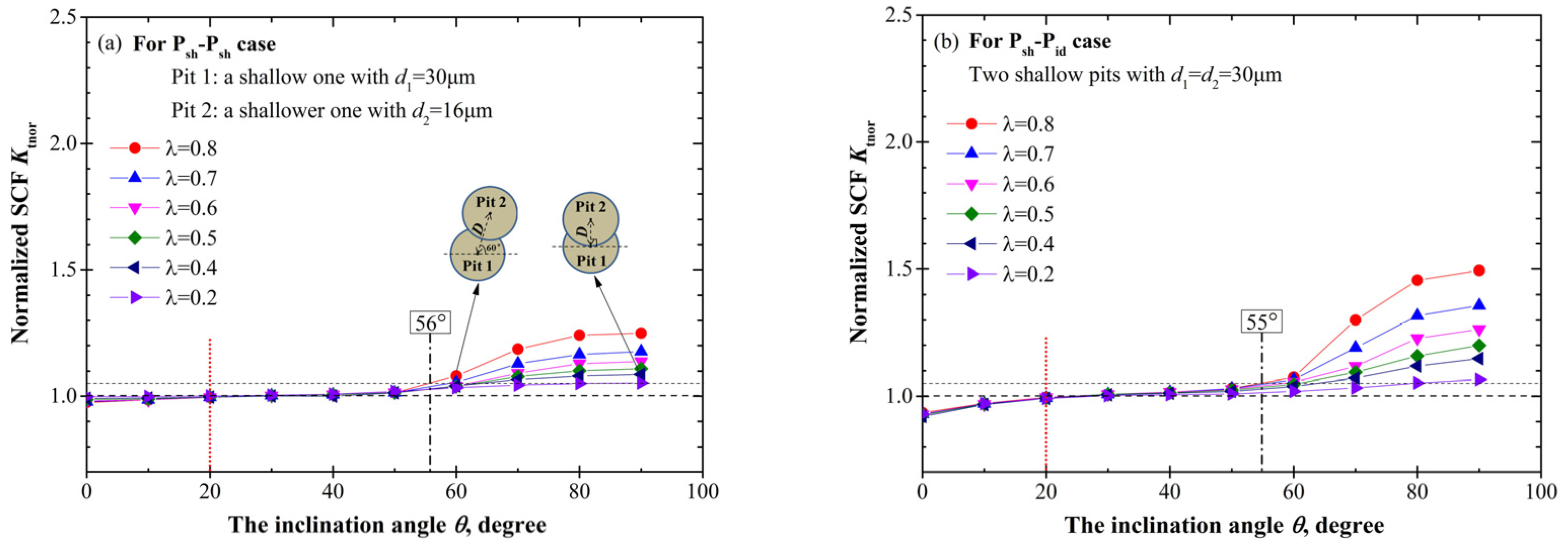
Figure 3 shows the variation of Ktnor with the relative position parameters θ and λ for six intersecting cases. Apparently, for all the cases Ktnor increases with the increase of the inclination angle θ as well as the dimensionless spacing parameter λ, and always, Ktnor reaches its maximum at θ = 90° for any λ discussed. Here, we define the inclination angle corresponding to the maximum Ktnor as the critical angle and denote it with θcri. Thus, for two intersecting pits the critical angle θcri is always 90°, which is a symmetric location for the two pits with respect to the loading direction.
By comparing the shallow cases (Figure 3a,b) to the hemi-spherical (Figure 3c,d) and deep cases (Figure 3e,f), it can be found that Ktnor increases with the increase of the pit depth. For the given spatial parameters λ = 0.8 and θ = 90°, Ktnor is about 1.25 for the shallow Psh-Psh case (Ktcom = 2.2), while for the deep Pde-Psh case Ktnor increases to about 2.31 (Ktcom = 5.8). The corresponding stress contours are given and compared in Figure 4, reflecting the higher stress concentration and the greater stress gradient for the deeper pits.
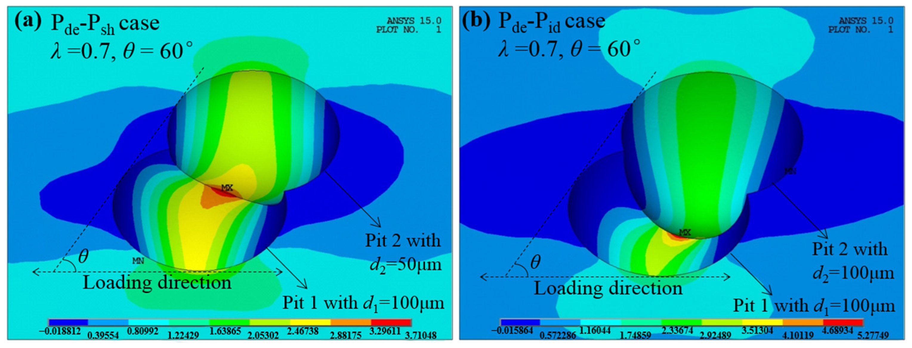
Furthermore, when comparing Figure 3a,c,e to Figure 3b,d,f respectively, it is clear that interacting effects are more pronounced for the two identical pits than those for the counterparts with a shallower pit, which is further graphically illustrated in Figure 5 with the stress contour of the Pde-Psh case (d1 = 100 μm, d2 = 50 μm) compared to that of the Pde-Pid case (d1 = 100 μm, d2 = 100 μm) when λ = 0.7 and θ = 60°. This feature implies that a neighboring pit whose size is roughly identical to the single pit can exert more influence on the stress field than a shallower one.
Another interesting phenomenon shown in Figure 3 is that θ = 20° (marked with the dot lines) looks like a turning point for interacting effects. When θ > 20°, Ktnor is greater than 1, i.e., Ktcom > Ktsin, which reflects the amplification effect on the stress concentration. When θ < 20°, Ktnor is less than 1, i.e., Ktcom < Ktsin, which indicates the relaxation effect on the stress concentration. Comparing Figure 3a,c,e to Figure 3b,d,f, the relaxation effect for the shallower cases is insignificant due to the lower influence induced by the shallower neighboring pit, thus Ktnor approximately remains 1 when θ < 20°.
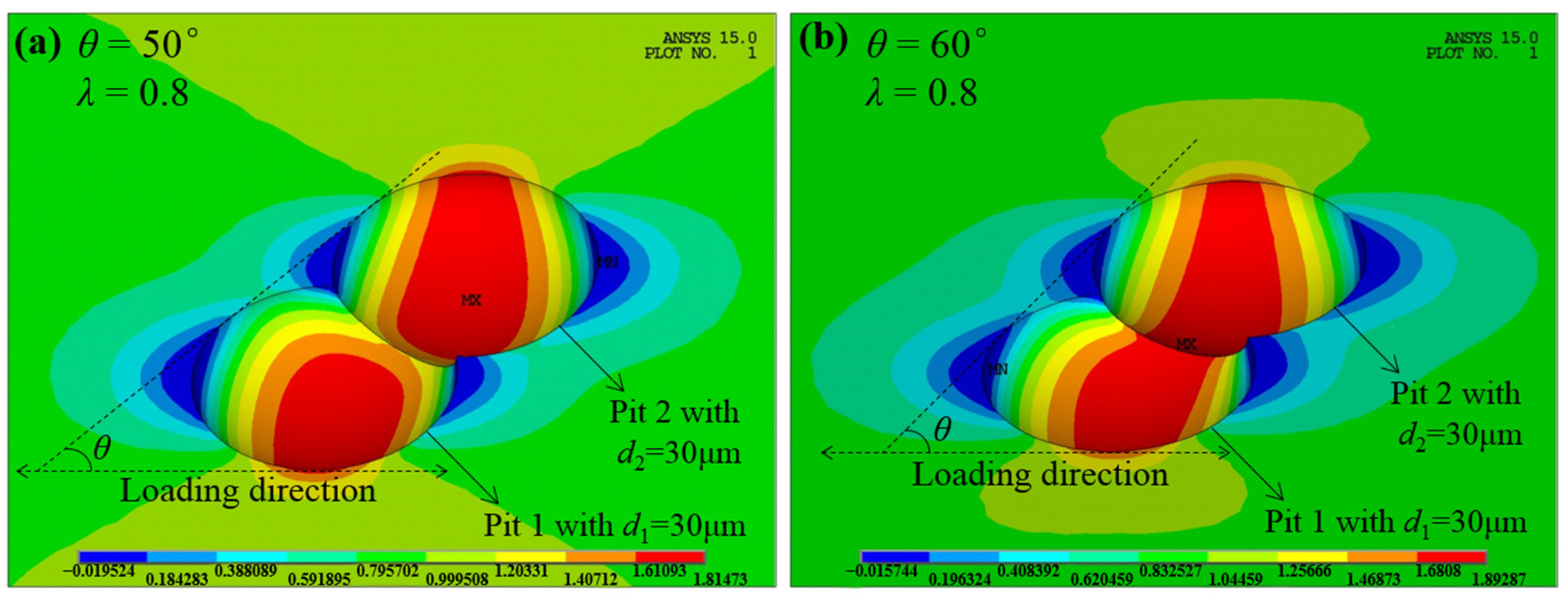
At the initial increase of θ from 20°, owing to such a slight growth of Ktnor, we assume that the amplification effect actually begins to work when the C-SCF increases by 5% over that of the single pit, and define the inclination angle corresponding to Ktnor = 1.05 as the threshold angle θth, as marked and labeled in Figure 3 for the limiting case of λ = 0.8. The comparison of stress contours with different θ is shown in Figure 6 for the Psh-Pid case (θth = 55°) when λ = 0.8. We can see that when θ < θth (50° in Figure 6a), the maximum C-SCF is located on the wall of Pit 2, and the stress distribution is almost the same with that of a single pit [4]. Yet when θ > θth (60° in Figure 6b), the maximum C-SCF will shift to the common separation wall between the two pits, which means that the neighboring pit begins to exert influence on the combined stress field.
3.1.2. Two Adjacent Pits
Contrary to intersecting cases, for adjacent pits the normalized SCF Ktnor decreases with the increase of the dimensionless spacing parameter λ, as shown in Figure 7. Moreover, when λ is greater than 2, Ktnor approximately remains 1 irrespective of any variation of θ, which is exemplified in Figure 8 with the stress contours at three different θ (10°, 45°, 90°) for the Pse-Pid case when λ = 2.5.
As shown in Figure 7 and Figure 8, when λ > 2, a neighboring pit will have little contribution to the stress concentration resulting from a single pit, which is in good accordance with the similar conclusions proposed for both pits [11,19] and cracks [23,24].
In broad terms, the variation tendency for Ktnor with the pit depth is similar to that for intersecting cases, but with a less pronounced increase for adjacent pits which can be attributed to the larger spacing between the two pits. In addition, the turning point θ = 20° and the threshold value θth exist for adjacent pits as well, and the decreasing trend of θth with the increase of the pit depth is nearly the same with that for intersecting pits. It should be noted that at the limiting case λ = 1.1, the θth for two identical shallow, hemi-spherical, and deep pits is 55°, 45°, and 30°, respectively, which correspondingly equals the counterpart for intersecting cases.
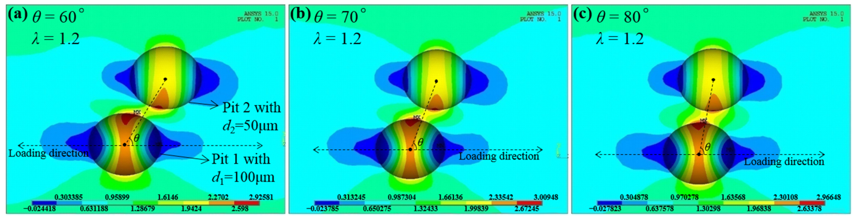
Unlike the monotonous relationship of Ktnor with θ for intersecting cases, for adjacent pits the maximum Ktnor does not always occur at the symmetric location which may be intuitively expected. Actually, only shallow cases (Figure 7a,b) with λ = 1.1 act like intersecting cases, i.e., Ktnor reaches its maximum at θcri = 90°. For all the other cases shown in Figure 7, Ktnor reaches its maximum at a slightly asymmetric location, such as θcri = 80° and θcri = 70°. Figure 9 presents the stress contours at θcri = 70° compared to those at θ = 60° and θ = 80° for the Pde-Psh case when λ = 1.2. It can be found that the maximum stress is located on the wall of Pit 1 near the common separation region, and the C-SCF reaches its maximum at θcri = 70°. It is interesting that the slight asymmetry will result in the maximum C-SCF, which has also been reported for cracks [25] and holes [26], i.e., the interaction effect reaches its maximum in the configuration where the symmetry is slightly perturbed instead of in the ideally symmetric arrangement. Yet the dependence of this asymmetry on the pit depth, as well as the spacing between two pits, has so far not been discussed.
As we can see from Figure 7, for a fixed λ, θcri slightly decreases with the increase of the pit depth. Taking two identical pits for an example, when λ = 1.1, θcri equals to 90°, 80°, and 70° for double shallow, hemi-spherical, and deep pits, respectively, which can be correspondingly observed in Figure 7b,d,e. The more accurate relationship of θcri and the pit depth will be discussed with more cases below.
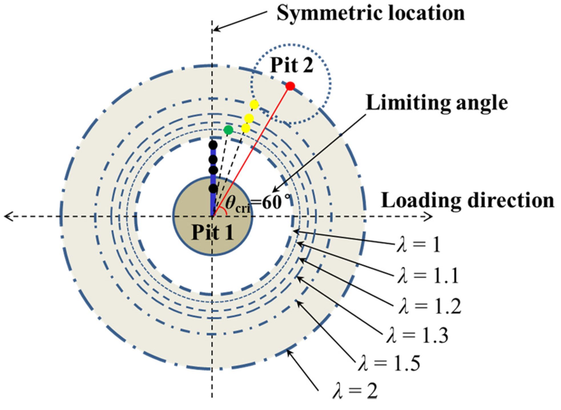
In addition, with the increasing of λ from 1.1 to 2, θcri generally decreases in the range of 60–80°. This tendency is illustrated explicitly with black orthogonal symbols in Figure 7d, that is, θcri = 80° for λ = 1.1, θcri = 70° for λ = 1.2, 1.3, and 1.5, and θcri = 60° for λ = 2. Together with the results for the intersecting pits (i.e., θcri = 90° for 0 < λ < 1), the variation tendency of θcri with λ can be schematically illustrated in Figure 10. The colored dot is used to point out the location of Pit 2. We can see that with the increase of the spacing between the two pits, the C-SCF will reach its maximum at θ deviating more from the symmetric location, and notably, the limiting angle will be θcri = 60° since there is almost no interacting effects between the two pits when λ > 2.
3.1.3. The Critical Corrosion Region
According to the severity of the C-SCF, we can summarize the influence of the relative position parameters and determine the critical corrosion region for Pit 2, which denotes the area with high susceptibility to fatigue damage due to the amplified C-SCF. Figure 11 gives the schematic illustration displaying the critical corrosion regions for both the intersecting and adjacent cases, where the dashed circle represents the possible location for Pit 2. With regard to the intersecting pits (0 < λ < 1), the C-SCF reaches its maximum at θcri = 90°, thus the colored band in Figure 11a corresponds to the critical corrosion region for Pit 2. While for adjacent cases (1 < λ ≤ 2), the maximum C-SCF occurs in the range of 60° ≤ θ ≤ 90° due to the asymmetric characteristic of θcri, thus the colored fan-shaped area in Figure 11b gives the critical corrosion region for Pit 2. It is worthwhile to mention that for the colored area, generally, the darker the stained band is, the higher the C-SCF is.
The obtained results for Ktnor’s variation with the relative position parameters may provide a mechanics-based explanation for the candidate locations of fatigue crack initiation. Medina et al. [27] observed in the experiments that maximum pit depth showed very low correlation with the location of fatigue fracture. They ascribed this phenomenon to the relaxation of the stress concentration caused by neighboring pits. With reference to our results, we believe that besides the reason mentioned in [27], the amplification effect on the stress concentration is another possible cause for this phenomenon. Figure 12 shows a typical fracture observed through scanning electron microscope (SEM) in our previous work [17]. The fatigue crack initiates from two intersecting pits with θ = 90° rather than the nearby deep pit, which can be attributed to the amplification effect on the combined stress concentration.
Furthermore, studies [22,28,29,30] have frequently mentioned that fatigue cracks originate from shallow pits rather than deep ones, and so far there is still no sound explanation for this phenomenon. According to our results, this observation may be attributed to the presence of an adjacent pit located in the critical region, especially when θ is in the range of 60°–70°, where the pit may remain invisible during conventional fracture analysis. A neighboring pit like that will induce such an increase in the C-SCF that even a shallow pit, that seems like a single one via SEM observation, can nucleate a fatigue crack and eventually lead to structural failure. This feature also implies that the conventional 2D SEM analysis is not enough to characterize the corrosion fatigue fracture due to interacting effects caused by neighboring pits, and 3D fracture analysis instead should be performed for better understanding of failure mechanisms.
3.2. The Influence of Pit Depth
As discussed before, the normalized SCF Ktnor is not only associated with the relative position parameters λ and θ, but also with the pit depth d. Based on the analysis in Section 3.1, the general characteristics of Ktnor’s variation with the pit depth have been initially observed by focusing on three settings, i.e., shallow, sphere, and deep pits. To further clarify the influence of the pit depth on the C-SCF, we append more FEA calculations with other pit depths regarding two identical neighboring pits. In addition, a dimensionless depth parameter Rd = d/r, also called the aspect ratio, is used in the following analysis for the purpose of generality.
3.2.1. The Relationship between θth and Pit Depth
As mentioned in Section 3.1.2, the threshold angle θth generally shows a decreasing trend with the increase of the pit depth, that is, θth is 55°, 45°, and 30° for double shallow (d = 30 μm), hemi-spherical (d = 50 μm), and deep pits (d = 100 μm), respectively. To further confirm this tendency, we perform FEA calculations at other depths with the limiting case of λ = 1.1, and determine the threshold angle θth according to the definition in Section 3.1.1. The calculation results are listed in Table 2 with the newly obtained θth shown in bold. It is noteworthy that the θth approaches 90° with the decrease of the pit depth, which suggests that the effect of neighboring pits on the stress concentration is nearly negligible for very shallow pits.
Figure 13 shows the decreasing tendency of θth with the increase of Rd, and their relationship can be expressed with an exponential decay function as,
Thus, when pit dimensions are obtained, the threshold angle θth can be conservatively estimated with Equation (3) since it is proposed regarding the limiting case of λ = 1.1.
3.2.2. The Relationship between Ktnor and Pit Depth
To better comprehend the dependence of Ktnor on the pit depth, supplementary calculations are performed for deeper pits with Rd = 1.6, 3, and 4 at the most disadvantaged configurations (i.e., the high stress concentration) of relative position parameters. Based on the results obtained in Section 3.1.1, for intersecting pits the most disadvantaged configuration is θ = 90° with λ = 0.8. All results of Ktnor at diverse pit depths are listed in Table 3 with the newly obtained results shown in bold.
For adjacent cases, the most disadvantaged spacing parameter is clearly λ = 1.1. Yet θcri varies with the pit depth, as initially discussed in Section 3.1.2. Thus, we add more FEA calculations for deeper pits in order to find not only the dependence of θcri on the pit depth, but also the variation of Ktnor with the pit depth. Table 4 lists the newly obtained results (in bold) as well as the results already obtained for d = 30 μm, 50 μm, and 100 μm. It can be found that for deeper pits, the maximum Ktnor always occurs at θcri = 70°. Since there is a slight difference of Ktnor between θcri = 90° and θ = 70° for the Psh-Pid case (1.27 vs. 1.19), as well as that between θcri = 80° and θ = 70° for the Pse-Pid case (1.43 vs. 1.39), we choose the case of λ = 1.1 with θ = 70° as the most disadvantageous configuration for two adjacent pits.
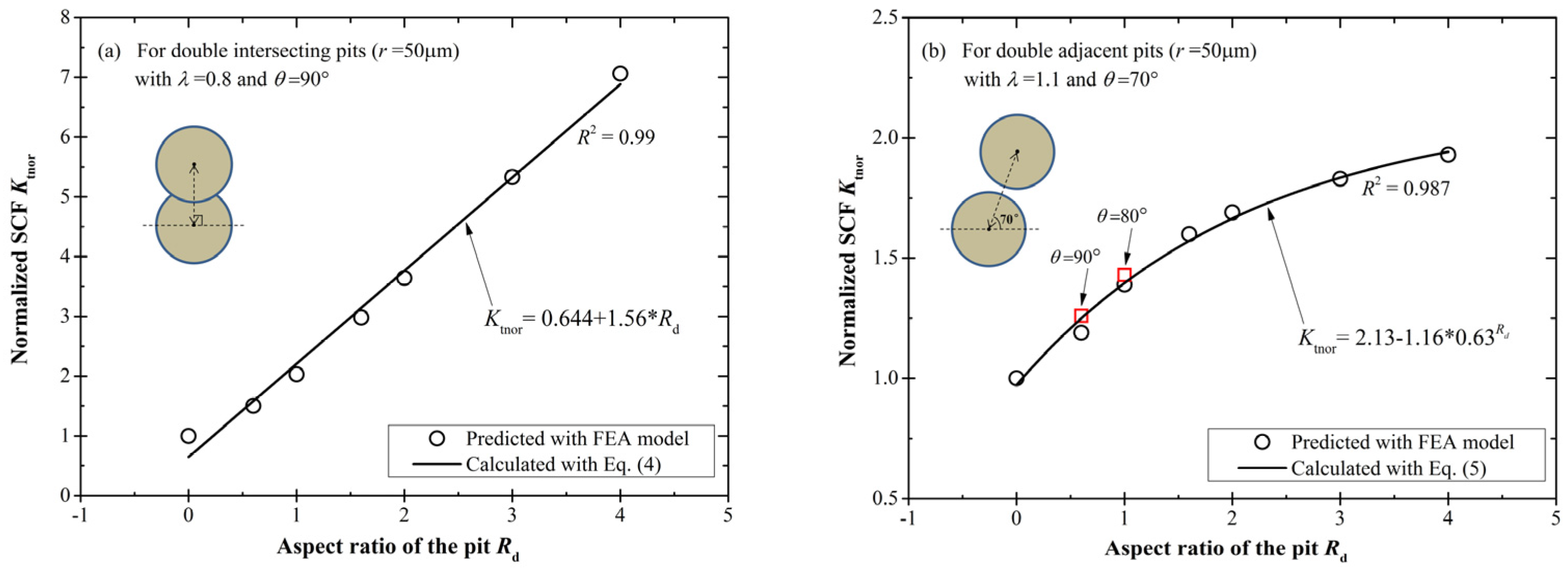
Figure 14 shows the relationship of the normalized SCF Ktnor vs. the aspect ratio Rd at the most disadvantageous configuration of the relative position parameters. For the intersecting case with λ = 0.8 and θ = 90° (Figure 14a), Ktnor presents good linearity with Rd and the linear growth can be given as,
This linear relationship reveals the strong dependence of Ktnor on the pit depth, and also implies that for intersecting cases, the pit depth is a highly sensitive parameter to which much attention should be paid. However, for the adjacent case with λ = 1.1 and θ = 70° (Figure 14b), Ktnor increases exponentially with Rd, and can be written as,
A declining tendency of the amplification effect can be observed with the increase of the pit depth, which suggests the weakened influence of the pit depth on the C-SCF for deeper adjacent pits.
In view of the above discussions, once we acquire the dimensions related to the pits, we can determine whether the interacting effects work on the stress field induced by the neighboring pits. Meanwhile, via the empirical formulas of Equations (4) or (5), we can conservatively estimate the combined SCF because they are proposed regarding to the most disadvantageous configuration of the relative position parameters. This convenient method to estimate the C-SCF is important for the structural safety assessment as well as for the structural design.
4. Application
4.1. Estimation Procedure for the C-SCF
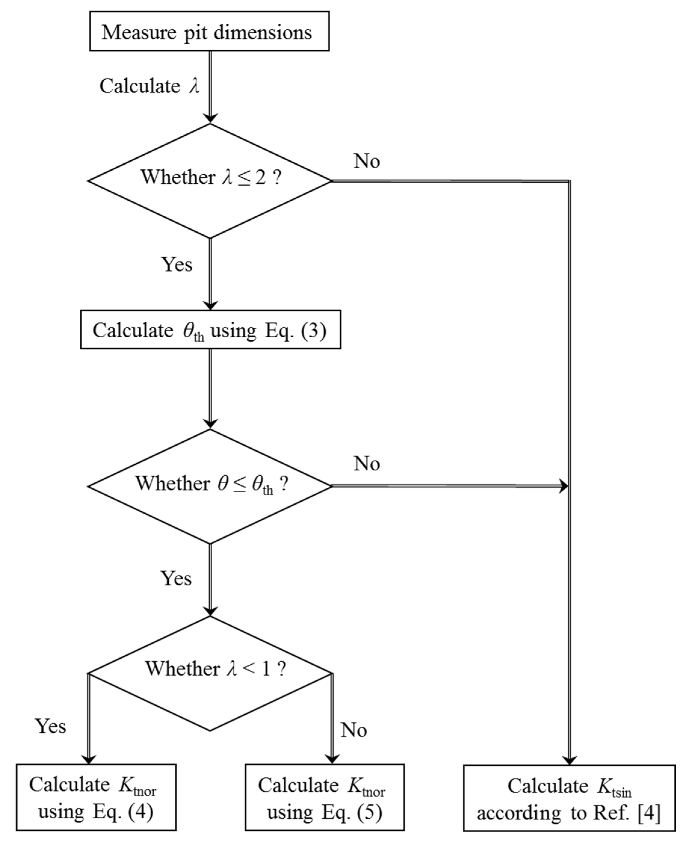
Figure 15 presents the flow chart to conservatively estimate the normalized SCF resulting from two neighboring pits. Firstly, the corrosion morphology is characterized to the obtain pit dimensions. Secondly, the dimensionless spacing parameter λ is calculated. If λ > 2, there is no significant interacting effect between these two pits, and it is recommended to estimate the SCF according to our previous work [4]. If λ ≤ 2, θth should be calculated using Equation (3). The third step is to examine whether the inclination angle θ of the two pits is greater than θth. Based on the discussion in Section 3.1.1, no interacting effect exists for θ < θth, and the SCF can be estimated according to [4]. If θ > θth, the spacing parameter λ should be further considered. If 0 < λ < 1, we calculate Ktnor by using the proposed formula of Equation (4), and otherwise, we predict Ktnor by using the proposed formula of Equation (5). Finally, the C-SCF Ktcom can be obtained through multiplying Ktnor by Ktsin, and the latter can be calculated using the method in [4].
4.2. Application Example
Full immersion corrosion tests are performed on an aluminum alloy 7075-T6 specimen in 3.5 wt % NaCl aqueous solution for 120 h. After pre-corrosion, the specimens are carefully rinsed in running water for 10 min and then dried.
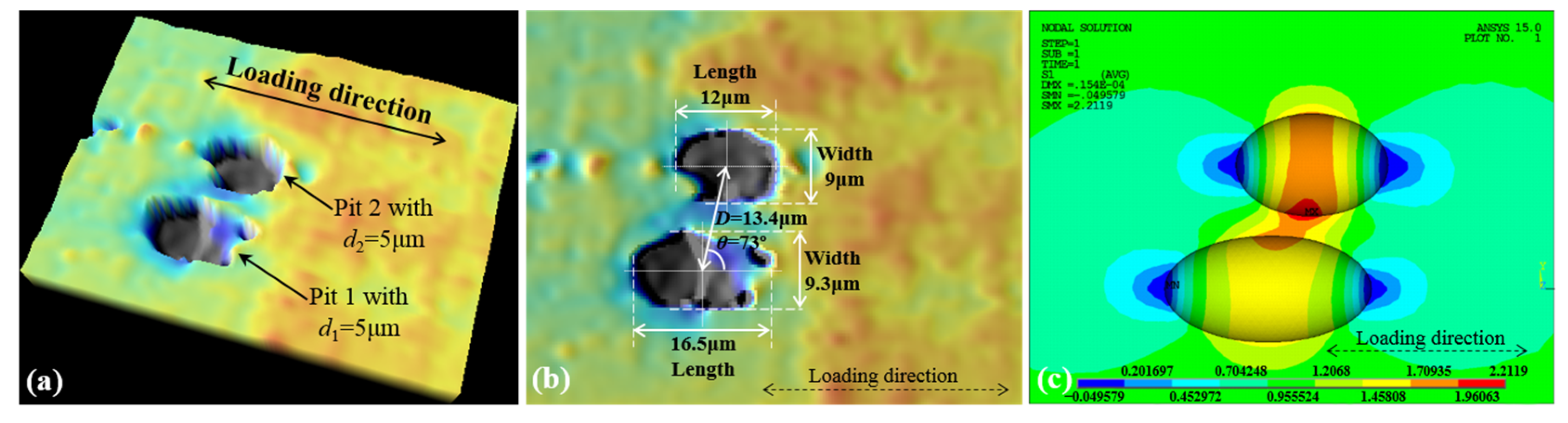
With a white light confocal microscope, two neighboring pits are characterized, and the obtained 3D and 2D morphology, as well as their pit dimensions, are shown in Figure 16a,b, respectively. In accordance with the measured dimensions, the FEA model is developed and the C-SCF is calculated. The stress contour is shown in Figure 16c, and the FEA calculation result for Ktcom is about 2.21.
To conservatively estimate the C-SCF, the elliptical pit is idealized as the one with a circular surface shape, i.e., r = 4.5 μm, since the latter has a slightly higher stress concentration effect than the former [4]. According to the measured dimensions, the dimensionless spacing parameter is λ = 13.4/9 ≈ 1.5, and is evidently less than 2. Then, we calculate the critical angle θth for these two pits by using Equation (3), and the result is θth = 43° with the aspect ratio Rd = 5/4.5 ≈ 1.11. As shown in Figure 16b, the measured inclination angle θ is 73°, and is apparently larger than θth. Therefore, the interacting effects will work on the stress field induced by Pit 1 and Pit 2, and the normalized SCF Ktnor can be estimated with Equation (5) proposed for two adjacent pits. By substituting Rd into the empirical formula, the achieved Ktnor is about 1.43.
With reference to our previous work [4], the SCF induced by a single pit (Ktsin) is about 2.12, thus the C-SCF can be predicted as the following,
Ktcom = Ktnor × Ktsin = 1.43 × 2.12 ≈ 3.03.
Compared to the FEA result (~2.21), the estimation error factor is about 1.37, which is mainly attributed to the conservative Ktnor calculated according to the most disadvantageous configuration of the relative position parameters. Additionally, the pit idealization, assuming the elliptical pit as the circular one, also introduces errors into the calculation of Ktsin and results in a larger value than the actual one (2.12 vs. 1.83 for the elliptical pit). The error factor of 1.37 may seem over-conservative. However, for circumstances where in-situ observations of pit dimensions are impossible or with worse accuracy, a relatively conservative estimation is usually needed and feasible for safety assessments. Therefore, the estimation method proposed here is still highly recommended given that a safety margin is always required to ensure the reliability of fatigue-related analysis and design.
5. Conclusions
By comprehensively considering the pit depth and the relative position parameters of two neighboring pits, their interacting effects on the stress concentration are analyzed and discussed. The noteworthy findings are summarized as follows,
- (1)
- For two intersecting pits, the combined SCF Ktcom increases with the increase of the relative position parameters θ and λ, and Ktcom always reaches its maximum at the symmetric location (θ = 90°) in the range of 0 < λ <1.
- (2)
- For two adjacent pits, the combined SCF Ktcom decreases with the increase of λ, and when λ > 2, the interacting effects have little contribution to the combined SCF, thus Ktcom ≈ Ktsin. The maximum C-SCF occurs at the asymmetric location of 60° ≤ θcri ≤ 90°. Meanwhile, θcri decreases with the increase of λ from 1 to 2, and θcri = 60° can be regarded as the limiting angle of this asymmetric feature.
- (3)
- The threshold angle θth exponentially decreases with the aspect ratio Rd (Equation (3)), which implies that the interacting effects induced by two neighboring pits exert influence in a larger scope for the deeper pits.
- (4)
- The normalized SCF generally increases with the pit depth, and follows a linear and an exponential relationship with Rd for two intersecting and adjacent pits, respectively. For the most disadvantageous configurations (i.e., the high stress concentration) of the relative position parameters, the empirical formulas (Equations (4) and (5)) are proposed to conservatively estimate the combined SCF and are validated via a practical example with the estimation error factor of 1.37.
In future work, pit eccentricity should be taken into account to further elucidate the interacting effect between two neighboring pits. In addition, a more complete study concerning a random arrangement of multi-pits will also be an interesting investigation.
Acknowledgments
The authors would like to thank the National Natural Science Foundation of China (No. 51475396), the National Basic Research Program of China (No. 2013CB733004), the Natural Scientific Research Innovation Foundation in Harbin Institute of Technology (No. 30620150071), the Fundamental Research Funds for the Central Universities (No. 20720170048) and the Scientific Project for Young and Middle-aged Teachers of Fujian Province (No. JAT160015) for their support.
Author Contributions
Yongfang Huang and Tieqiang Gang conceived and performed the simulations; Tieqiang Gang performed the experiments; Yongfang Huang analyzed the data; Lijie Chen contributed experimental materials and analysis tools; Yongfang Huang wrote the paper; and all the authors revised the paper together.
Conflicts of Interest
The authors declare no conflict of interest.
References
- Jones, K.; Hoeppner, D.W. Prior corrosion and fatigue of 2024-T3 aluminum alloy. Corros. Sci. 2006, 48, 3109–3122. [Google Scholar] [CrossRef]
- Kazempour-Liacy, H.; Mehdizadeh, M.; Akbari-Garakani, M.; Abouali, S. Corrosion and fatigue failure analysis of a forced draft fan blade. Eng. Fail. Anal. 2011, 18, 1193–1202. [Google Scholar] [CrossRef]
- Sharma, M.M.; Zeimian, C.W. Pitting and stress corrosion cracking susceptibility of nanostructured Al–Mg alloys in natural and artificial environments. J. Mater. Eng. Perform 2008, 1059, 94–95. [Google Scholar] [CrossRef]
- Huang, Y.F.; Wei, C.; Chen, L.J.; Li, P.F. Quantitative correlation between geometric parameters and stress concentration of corrosion pits. Eng. Fail. Anal. 2014, 44, 168–178. [Google Scholar] [CrossRef]
- Cerit, M. Numerical investigation on torsional stress concentration factor at the semi elliptical corrosion pit. Corros. Sci. 2013, 67, 225–232. [Google Scholar] [CrossRef]
- Burns, J.T.; Larsen, J.M.; Gangloff, R.P. Driving forces for localized corrosion-to-fatigue crack transition in Al–Zn–Mg–Cu. Fatigue Fract. Eng. Mater. Struct. 2011, 34, 745–773. [Google Scholar] [CrossRef]
- Turnbull, A.; Wright, L.; Crocker, L. New insight into the pit-to-crack transition from finite element analysis of the stress and strain distribution around a corrosion pit. Corros. Sci. 2010, 52, 1492–1498. [Google Scholar] [CrossRef]
- Cerit, M.; Genel, K.; Eksi, S. Numerical investigation on stress concentration of corrosion pit. Eng. Fail. Anal. 2009, 16, 2467–2472. [Google Scholar] [CrossRef]
- Pidaparti, R.M.; Patel, R.R. Correlation between corrosion pits and stresses in Al alloys. Mater. Lett. 2008, 62, 4497–4499. [Google Scholar] [CrossRef]
- Pao, P.S.; Gill, S.J.; Feng, C.R. On fatigue crack initiation from corrosion pits in 7075-T7351 aluminum alloy. Scr. Mater. 2000, 43, 391–396. [Google Scholar] [CrossRef]
- Domínguez Almaraz, G.M.; Mercada Lemus, V.H.; Villalón López, J.J. Effect of proximity and dimension of two artificial pitting holes on the fatigue endurance of aluminum alloy AISI 6061-T6 under rotating bending fatigue tests. Metall. Mater. Trans. A 2011, 43, 2271–2776. [Google Scholar] [CrossRef]
- Han, C.J.; Zhang, H.; Zhang, J. Failure pressure analysis of the pipe with inner corrosion defects by FEM. Int. J. Electrochem. Sci. 2016, 11, 5046–5062. [Google Scholar] [CrossRef]
- Kolios, A.; Srikanth, S.; Salonitis, K. Numerical simulation of material strength deterioration due to pitting corrosion. Procedia CIRP 2014, 13, 230–236. [Google Scholar] [CrossRef]
- Hou, J.; Song, L. Numerical investigation on stress concentration of tension steel bars with one or two corrosion pits. Adv. Mater. Sci. Eng. 2015, 1–7. [Google Scholar] [CrossRef]
- Pidaparti, R.M.; Rao, A.S. Analysis of pits induced stresses due to metal corrosion. Corros. Sci. 2008, 50, 1932–1938. [Google Scholar] [CrossRef]
- Xu, Y.D. The Corrosion characteristics and tensile behavior of reinforcement under coupled carbonation and static loading. Materials 2015, 8, 8561–8577. [Google Scholar] [CrossRef]
- Huang, Y.F.; Ye, X.B.; Hu, B.R.; Chen, L.J. Equivalent crack size model for pre-corrosion fatigue life prediction of aluminum alloy 7075-T6. Int. J. Fatigue 2016, 88, 217–226. [Google Scholar] [CrossRef]
- Huang, Y.F. Fatigue Testing and Life Prediction for Pre-Corroded Aluminum Alloy 7075-T6. Ph.D. Thesis, Xiamen University, Xiamen, China, 2014. (In Chinese). [Google Scholar]
- Van der Walde, K. Corrosion-Nucleated Fatigue Crack Growth. Ph.D. Thesis, Purdue University, West Lafayette, IN, USA, 2005. [Google Scholar]
- Huang, Y.F.; Chen, L.J.; Ye, X.B. Statistical analysis of pit dimensions for pre-corroded AA7075-T6. Adv. Mater. Res. 2014, 906, 259–262. [Google Scholar] [CrossRef]
- Pistorius, P.C.; Burstein, G.T. Metastable pitting corrosion of stainless steel and the transition to stability. Phil. Trans. R. Soc. Lond. A 1992, 341, 531–559. [Google Scholar] [CrossRef]
- Medved, J.J.; Breton, A.M.; Irving, P.E. Corrosion pit size distributions and fatigue lives—A study of the EIFS technique for fatigue design in the presence of corrosion. Int. J. Fatigue 2004, 26, 71–80. [Google Scholar] [CrossRef]
- Kishimoto, K.; Soboyejo, W.O.; Smith, R.A.; Knott, J.F. A numerical investigation of the interaction and coalescence of twin coplanar semi-elliptical fatigue cracks. Int. J. Fatigue 1989, 11, 91–96. [Google Scholar] [CrossRef]
- Noda, N.-A.; Kobayashi, K.; Oohashi, T. Variation of the stress intensity factor along the crack front of interacting semi-elliptical surface cracks. Arch. Appl. Mech. 2001, 71, 43–52. [Google Scholar] [CrossRef]
- Kachanov, M. Elastic solids with many cracks and related problems. In Advances in Applied Mechanics; Hutchinson, J.W., Wu, T.Y., Eds.; Academic Press: New York, NY, USA, 1993; Volume 3, pp. 259–445. [Google Scholar]
- Tsukrov, I.; Kachanov, M. Stress concentrations and microfracturing patterns in a brittle-elastic solid with interacting pores of diverse shapes. Int. J. Solids Struct. 1997, 34, 2887–2904. [Google Scholar] [CrossRef]
- Medina, H.; Hinderliter, B. Where do random rough surfaces fail? Part I: Fracture loci safety envelopes at early stages of degradation. J. Energy Power Eng. 2013, 7, 907–916. [Google Scholar]
- Kim, S.; Burns, J.T.; Gangloff, R.P. Fatigue crack formation and growth from localized corrosion in Al-Zn-Mg-Cu. Eng. Fract. Mech. 2009, 76, 651–667. [Google Scholar] [CrossRef]
- Crawford, B.R.; Sharp, P.K. Equivalent Crack Size Modelling of Corrosion Pitting in an AA7050-T7451 Aluminium Alloy and Its Implications for Aircraft Structural Integrity; Technical Report; DSTO-TR-2745: Melbourne, Victoria, Australia, 2012. [Google Scholar]
- Gruenberg, K.M.; Craig, B.A.; Hillberry, B.M.; Bucci, R.J.; Hinkle, A.J. Predicting fatigue life of pre-corroded 2024-T3 aluminum. Int. J. Fatigue 2004, 26, 629–640. [Google Scholar] [CrossRef]
Figure 1.
Details of the model containing two neighboring pits. (a) Sketch outline of the adjacent and intersecting cases; and (b) diagram of the configurations of Pit 1 and Pit 2.
Figure 1.
Details of the model containing two neighboring pits. (a) Sketch outline of the adjacent and intersecting cases; and (b) diagram of the configurations of Pit 1 and Pit 2.
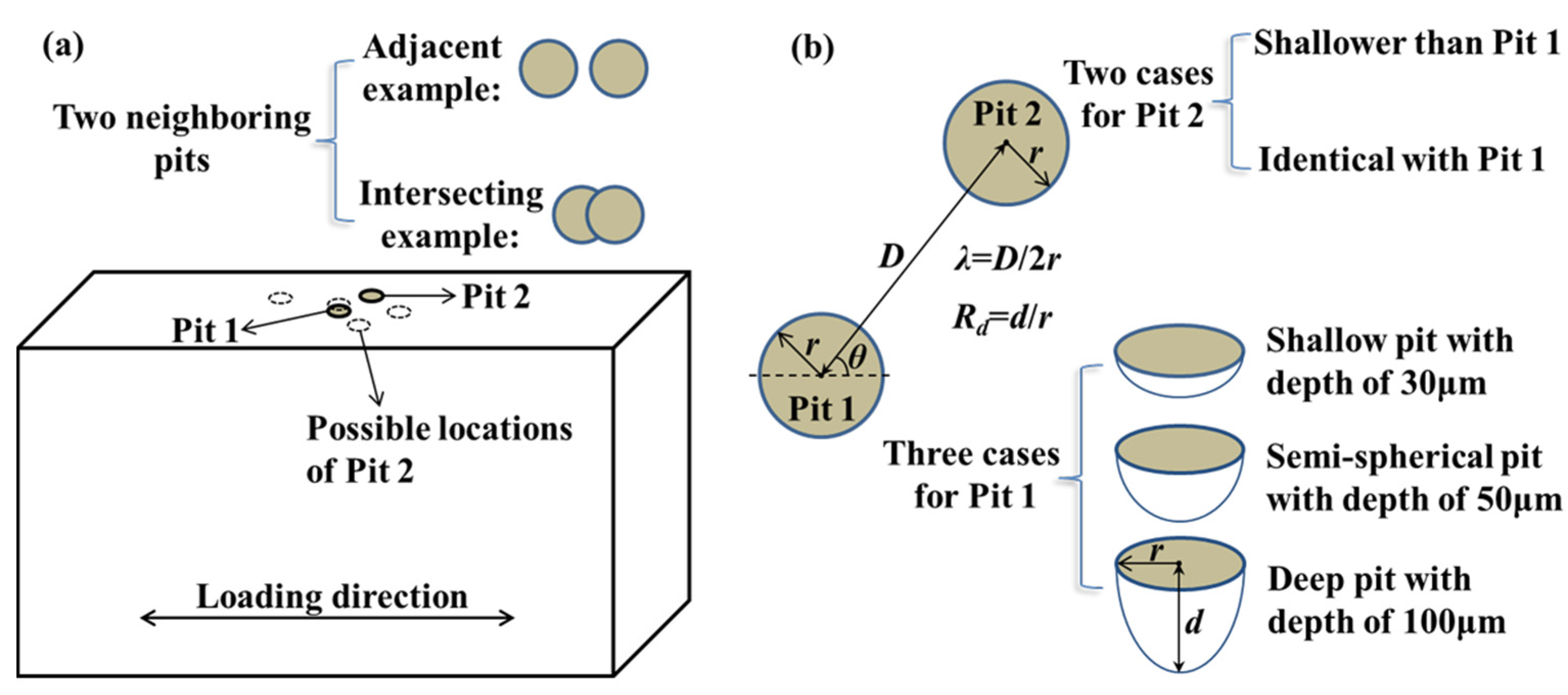
Figure 2.
The results of finite element meshing and the convergence study. (a) The mesh refinement around the pits with the inset showing the whole model meshes; and (b) the convergence study with different numbers of elements.
Figure 2.
The results of finite element meshing and the convergence study. (a) The mesh refinement around the pits with the inset showing the whole model meshes; and (b) the convergence study with different numbers of elements.
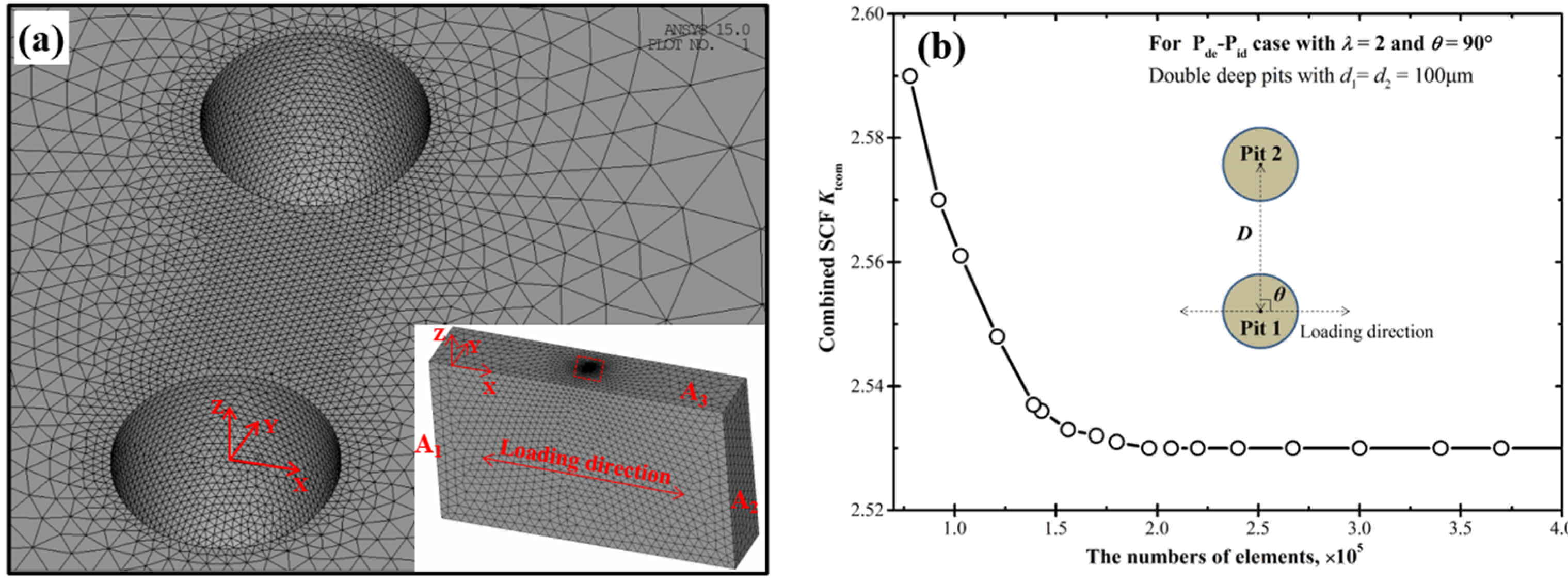
Figure 3.
The variation of Ktnor with the relative position parameters λ and θ for two intersecting pits. (a) Psh-Psh case; (b) Psh-Pid case; (c) Pse-Psh case; (d) Pse-Pid case; (e) Pde-Psh case; and (f) Pde-Pid case.
Figure 3.
The variation of Ktnor with the relative position parameters λ and θ for two intersecting pits. (a) Psh-Psh case; (b) Psh-Pid case; (c) Pse-Psh case; (d) Pse-Pid case; (e) Pde-Psh case; and (f) Pde-Pid case.

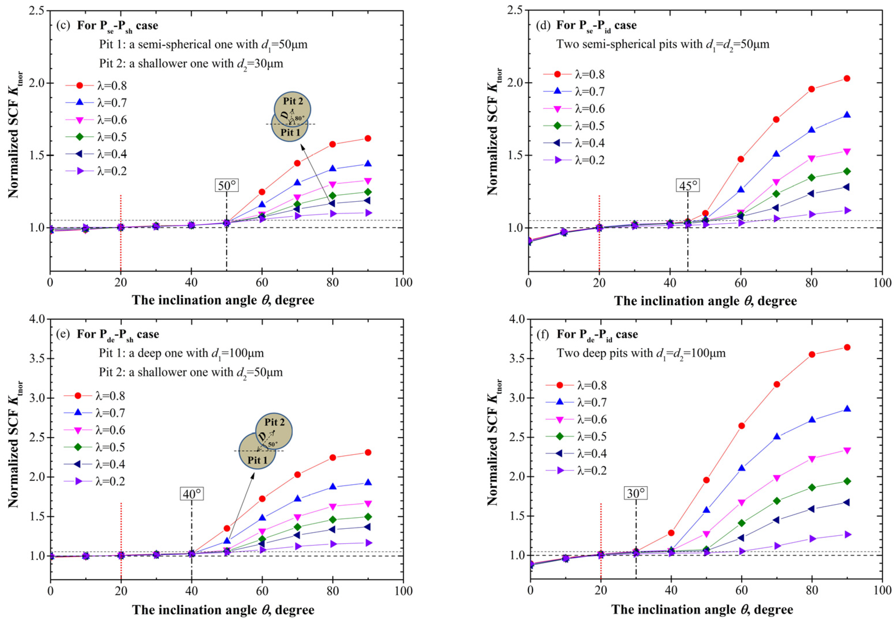
Figure 4.
The comparison of stress contours with different pit depths. (a) d1 = 30 μm, d2 = 16 μm; and (b) d1 = 100 μm, d2 = 50 μm. The units of stress in this and the subsequent figures are MPa.
Figure 4.
The comparison of stress contours with different pit depths. (a) d1 = 30 μm, d2 = 16 μm; and (b) d1 = 100 μm, d2 = 50 μm. The units of stress in this and the subsequent figures are MPa.
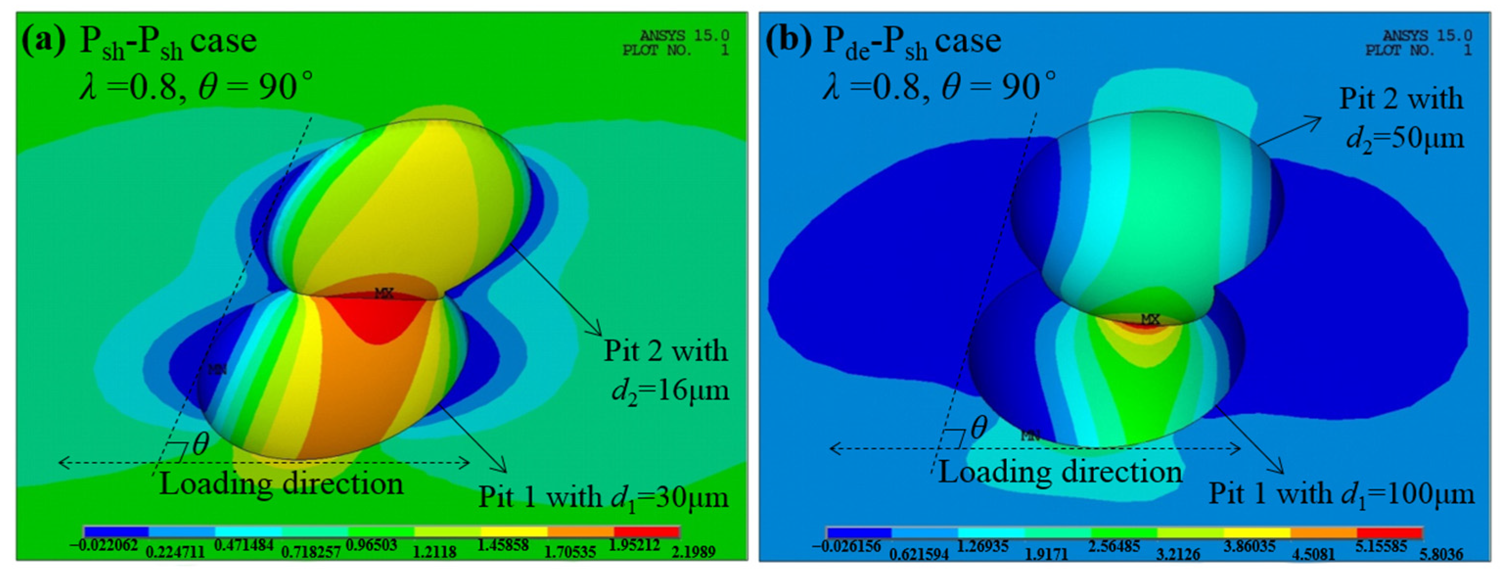
Figure 5.
The comparison of stress contours with different depths of Pit 2. (a) d1 = 100 μm, d2 = 50 μm; and (b) d1 = 100 μm, d2 = 100 μm.
Figure 5.
The comparison of stress contours with different depths of Pit 2. (a) d1 = 100 μm, d2 = 50 μm; and (b) d1 = 100 μm, d2 = 100 μm.

Figure 6.
The comparison of stress contours with different inclination angle θ for the Psh-Pid case (d1 = d2 = 30 μm) when λ = 0.8 and θth = 55°. (a) θ < θth; and (b) θ > θth.
Figure 6.
The comparison of stress contours with different inclination angle θ for the Psh-Pid case (d1 = d2 = 30 μm) when λ = 0.8 and θth = 55°. (a) θ < θth; and (b) θ > θth.

Figure 7.
The variation of Ktnor with the relative position parameters λ and θ for two adjacent pits. (a) Psh-Psh case; (b) Psh-Pid case; (c) Pse-Psh case; (d) Pse-Pid case; (e) Pde-Psh case; and (f) Pde-Pid case.
Figure 7.
The variation of Ktnor with the relative position parameters λ and θ for two adjacent pits. (a) Psh-Psh case; (b) Psh-Pid case; (c) Pse-Psh case; (d) Pse-Pid case; (e) Pde-Psh case; and (f) Pde-Pid case.
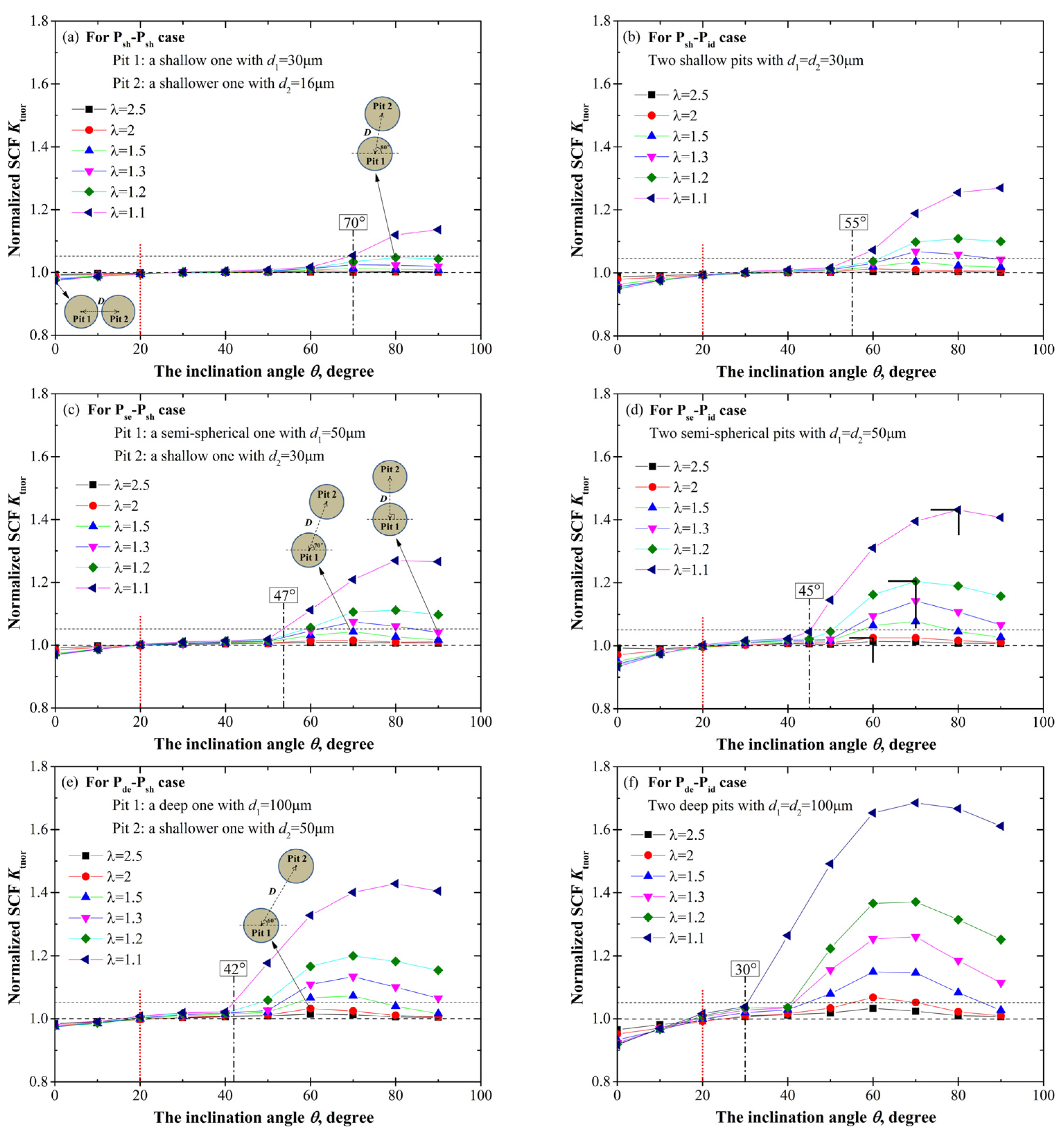
Figure 8.
The comparison of stress contours with different θ for the Pse-Pid case (d1 = d2 = 50 μm) when λ = 2.5, showing little interacting effect between these two pits. (a) For θ = 10°; (b) for θ = 45°; and (c) for θ = 90°.
Figure 8.
The comparison of stress contours with different θ for the Pse-Pid case (d1 = d2 = 50 μm) when λ = 2.5, showing little interacting effect between these two pits. (a) For θ = 10°; (b) for θ = 45°; and (c) for θ = 90°.
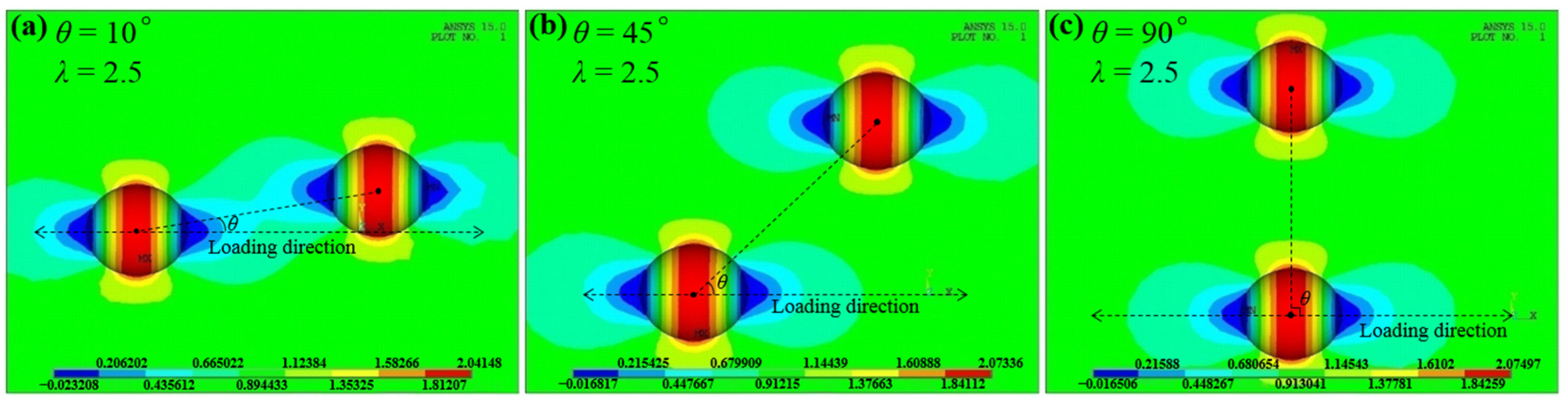
Figure 9.
The comparison of stress contours with different θ for the Pde-Psh case (d1 = 100 μm, d2 = 50 μm) when λ = 1.2, showing the slight asymmetric characteristic that results in the maximum C-SCF (combined stress concentration factor). (a) For θ = 60°; (b) for θ = 70°; and (c) for θ = 80°.
Figure 9.
The comparison of stress contours with different θ for the Pde-Psh case (d1 = 100 μm, d2 = 50 μm) when λ = 1.2, showing the slight asymmetric characteristic that results in the maximum C-SCF (combined stress concentration factor). (a) For θ = 60°; (b) for θ = 70°; and (c) for θ = 80°.

Figure 10.
Schematic drawing showing the relationship of θcri with λ, reflecting the dependence of the asymmetry feature on the spacing between two pits. For clarity, the locations of Pit 2 are presented with colored dots. The black, green, yellow, and red dots correspond to 90°, 80°, 70° and 60°, respectively.

Figure 11.
Diagram showing the critical corrosion region for a neighboring pit. The dashed circle represents the possible location for Pit 2, and the colored area corresponds to the critical corrosion region, with the darker color illustrating the higher C-SCF. (a) For intersecting pits; and (b) for adjacent pits. Notably, for a fixed λ in Figure 11b, the C-SCF slightly varies with the inclination angle θ, which is schematically illustrated with the color gradients in each stained band.

Figure 12.
Typical SEM fractography with the fatigue crack initiating from two intersecting pits rather than the deeper pit. (a) Overall view of the fracture surface; and (b) local view of the crack origin.
Figure 12.
Typical SEM fractography with the fatigue crack initiating from two intersecting pits rather than the deeper pit. (a) Overall view of the fracture surface; and (b) local view of the crack origin.
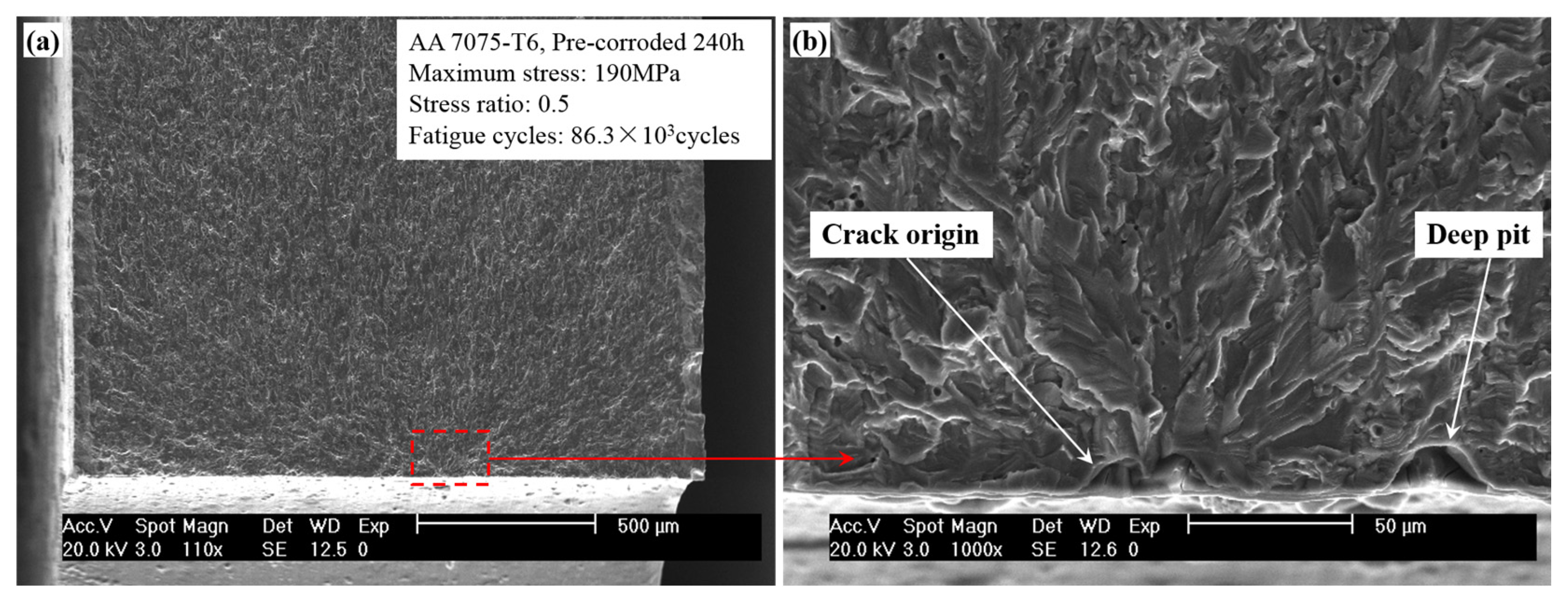
Figure 13.
The relationship of the threshold angle θth with the aspect ratio Rd, reflecting the dependence of the affected spatial scope on the pit depth.
Figure 13.
The relationship of the threshold angle θth with the aspect ratio Rd, reflecting the dependence of the affected spatial scope on the pit depth.
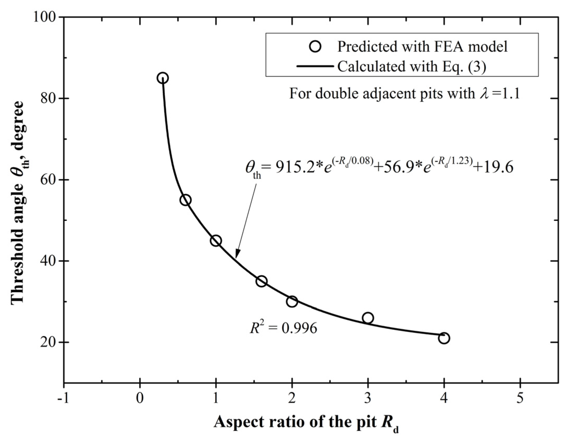
Figure 14.
The relationship of the normalized SCF Ktnor with the aspect ratio Rd at the most disadvantageous configuration (i.e., the high stress concentration) of the relative position parameters. (a) For intersecting pits; and (b) for adjacent pits.
Figure 14.
The relationship of the normalized SCF Ktnor with the aspect ratio Rd at the most disadvantageous configuration (i.e., the high stress concentration) of the relative position parameters. (a) For intersecting pits; and (b) for adjacent pits.

Figure 15.
Flow chart for estimating the normalized SCF.

Figure 16.
An example for corrosion characterization and the FEA (finite element analysis) result of the C-SCF. (a) 3D morphology; (b) 2D morphology with pit dimensions; and (c) the FEA result for the C-SCF.
Figure 16.
An example for corrosion characterization and the FEA (finite element analysis) result of the C-SCF. (a) 3D morphology; (b) 2D morphology with pit dimensions; and (c) the FEA result for the C-SCF.


Table 1.
The definitions and settings for the configurations of Pit 1 and Pit 2.
| Definition | Pit 2 (μm) | ||
|---|---|---|---|
| Shallower | Identical | ||
| Pit 1 (μm) | Shallow | Psh-Psh (d1 = 30, d2 = 16) | Psh-Pid (d1 = 30, d2 = 30) |
| Hemi-spherical | Pse-Psh (d1 = 50, d2 = 30) | Pse-Pid (d1 = 50, d2 = 50) | |
| Deep | Pde-Psh (d1 = 100, d2 = 50) | Pde-Pid (d1 = 100, d2 = 100) | |
Table 2.
The results of θth for double adjacent pits (λ = 1.1) with various pit depths. The newly obtained ones are presented in bold.
Table 2.
The results of θth for double adjacent pits (λ = 1.1) with various pit depths. The newly obtained ones are presented in bold.
| d (μm) | Rd | Ktsin | Ktnor | θ |
|---|---|---|---|---|
| 15 | 0.3 | 1.53 | 1.051 | 86° |
| 1.047 | 85° | |||
| 30 | 0.6 | 1.76 | 1.05 | 55° |
| 50 | 1 | 2.06 | 1.05 | 45° |
| 80 | 1.6 | 2.37 | 1.057 | 36° |
| 1.033 | 35° | |||
| 100 | 2 | 2.51 | 1.05 | 30° |
| 150 | 3 | 2.72 | 1.051 | 27° |
| 1.048 | 26° | |||
| 200 | 4 | 2.82 | 1.052 | 22° |
| 1.046 | 21° |
Table 3.
The results of Ktnor at diverse pit depths for double intersecting pits with λ = 0.8 and θ = 90°. The supplementary results are shown in bold.
Table 3.
The results of Ktnor at diverse pit depths for double intersecting pits with λ = 0.8 and θ = 90°. The supplementary results are shown in bold.
| d (μm) | Rd | Ktsin | Ktnor |
|---|---|---|---|
| 30 | 0.6 | 1.76 | 1.49 |
| 50 | 1 | 2.06 | 2.03 |
| 80 | 1.6 | 2.37 | 2.98 |
| 100 | 2 | 2.51 | 3.64 |
| 150 | 3 | 2.72 | 5.33 |
| 200 | 4 | 2.82 | 7.062 |
Table 4.
The variation of Ktnor and θcri with the pit depths for double adjacent pits when λ = 1.1. The supplementary results are listed in bold.
Table 4.
The variation of Ktnor and θcri with the pit depths for double adjacent pits when λ = 1.1. The supplementary results are listed in bold.
| d (μm) | Rd | Ktsin | Ktnor | θ |
|---|---|---|---|---|
| 30 | 0.6 | 1.76 | 1.27 | 90° |
| 1.19 | 70° | |||
| 50 | 1 | 2.06 | 1.43 | 80° |
| 1.39 | 70° | |||
| 80 | 1.6 | 2.37 | 1.591 | 75° |
| 1.602 | 70° | |||
| 1.561 | 65° | |||
| 100 | 2 | 2.51 | 1.69 | 70° |
| 150 | 3 | 2.72 | 1.782 | 72° |
| 1.83 | 70° | |||
| 1.786 | 65° | |||
| 200 | 4 | 2.82 | 1.89 | 72° |
| 1.934 | 70° | |||
| 1.877 | 65° |
© 2017 by the authors. Licensee MDPI, Basel, Switzerland. This article is an open access article distributed under the terms and conditions of the Creative Commons Attribution (CC BY) license (http://creativecommons.org/licenses/by/4.0/).
Share and Cite
MDPI and ACS Style
Huang, Y.; Gang, T.; Chen, L. Interacting Effects Induced by Two Neighboring Pits Considering Relative Position Parameters and Pit Depth. Materials 2017, 10, 398. https://doi.org/10.3390/ma10040398
AMA Style
Huang Y, Gang T, Chen L. Interacting Effects Induced by Two Neighboring Pits Considering Relative Position Parameters and Pit Depth. Materials. 2017; 10(4):398. https://doi.org/10.3390/ma10040398
Chicago/Turabian StyleHuang, Yongfang, Tieqiang Gang, and Lijie Chen. 2017. "Interacting Effects Induced by Two Neighboring Pits Considering Relative Position Parameters and Pit Depth" Materials 10, no. 4: 398. https://doi.org/10.3390/ma10040398
Note that from the first issue of 2016, this journal uses article numbers instead of page numbers. See further details here.