Comparative Study of Hybrid Models Based on a Series of Optimization Algorithms and Their Application in Energy System Forecasting

Abstract

Big data mining, analysis, and forecasting play vital roles in modern economic and industrial fields, especially in the energy system. Inaccurate forecasting may cause wastes of scarce energy or electricity shortages. However, forecasting in the energy system has proven to be a challenging task due to various unstable factors, such as high fluctuations, autocorrelation and stochastic volatility. To forecast time series data by using hybrid models is a feasible alternative of conventional single forecasting modelling approaches. This paper develops a group of hybrid models to solve the problems above by eliminating the noise in the original data sequence and optimizing the parameters in a back propagation neural network. One of contributions of this paper is to integrate the existing algorithms and models, which jointly show advances over the present state of the art. The results of comparative studies demonstrate that the hybrid models proposed not only satisfactorily approximate the actual value but also can be an effective tool in the planning and dispatching of smart grids.

1. Introduction

The energy system is a complex system that achieves the simultaneous generation, transportation, distribution and consumption of electrical energy, playing a pivotal role in each field of social production. It is essential that the electrical power system have sufficient capacity to address dynamic change, which could otherwise affect the quality of the power supply and even endanger the safety and stability of the electrical system. Currently, the control of electrical systems helps to plan electricity management, arrange reasonable operation modes, save energy, reduce the costs of generating electricity and enhance both economic and social benefits [1]. Three indicators in the electrical system are crucial for adapting to modern and scientific power grid management: short-term wind speed, electrical load and electricity price because they are connected to generation, distribution and consumption, respectively.

First, the short-term wind speed can have a great influence on the generation of electricity. Faced with resource shortages, environmental pollution and ecosystem degradation, developing and utilizing clean energy with high efficiency has become an important topic. Wind is a clean and inexhaustible type of energy and one of the most promising energy resources [1]. Wind energy has achieved rapid development worldwide, and, as shown in Figure 1, the newly increased wind power installed capability has reached 51477 MW. The power of wind is proportional to the wind speed; therefore, the wind speed determines the magnitude of the wind power. Compared with the long- and middle-term wind speed, the randomness, fluctuation and intermittent nature of short-term wind speed makes it more difficult to control wind turbines or ensure the normal operation of the power grid [2]. Second, with the continuous increase in the installed capacity and the consumption of electrical power, forecasting the electrical load becomes more and more significant [3]. Electrical load forecasting means to estimate and forecast the electricity demand through analysing and researching the historical data and extracting the inner relationship of data from the perspective of known economic and social development and the demands of the electrical system, considering factors such as politics, economy and climate. In recent years, large-scale power outages in large-scale areas have been caused by extra electrical load, resulting in great economic losses [4]. Thus, the scientific control of electrical load seems vital. Finally, the indicator electricity price is related to its consumption, which can be adjusted with changes in supply and demand until it tends to be reasonable. Forecasting the electricity price is crucial because it has already become one of the cores of electricity marketization [5]. On the one hand, the electricity price could balance the economic interests of participants in the market. On the other hand, the market would also be faced with large risks in electricity price owing to the fluctuation of the wind [6].

Based on the discussion above, we can see that forecasting the electrical power system with high accuracy and reliability is a widespread difficulty; however, it is of great significance. Based on the computational mechanism, the forecasting methods can be divided into four types: statistical methods, physical methods, intelligent methods and hybrid methods.

1.1. Statistical Forecasting Methods

Statistical methods construct mathematical and statistical models to conduct time series forecasting and offer better real-time performance [7]. Statistical forecasting methods achieve reduced forecasting errors if the input variables are under normal conditions [8]. Autoregressive integrated moving average (ARIMA) is a typical statistical technique that is widely used in time series forecasting. Kavasseri and Seetharaman [9] examined the use of a fractional-ARIMA model to forecast wind speeds on the day-ahead and two-day-ahead horizons. The forecast errors in wind speed were analysed and compared with the persistence model, and the results indicated significant improvements in forecasting accuracy. Wang et al. [10] proposed residual modification models to improve the precision of seasonal ARIMA for electricity demand forecasting. They applied a seasonal ARIMA approach, an optimal Fourier method optimized by particle swarm optimization (PSO) and combined the PSO optimal Fourier method with seasonal ARIMA to correct the forecasting results for electrical power in northwest China. The final results showed that the forecasting accuracy was higher than the seasonal ARIMA model alone and that the combined model was the most satisfactory. Shukur and Lee [11] stated that the non-linearity in the patterns of wind speed data was the reason for inaccurate wind speed forecasting using a linear ARIMA model, and the inaccurate forecasting of the ARIMA model reflected the uncertainty of the modelling process. Babu and Reddy [12] explored both linear ARIMA and non-linear artificial neural network (ANN) models to devise a new hybrid ARIMA-ANN model for the forecasting of electricity price. Cadenas and Rivera [13] also combined ARIMA and ANN for wind speed forecasting using measured hourly wind speed time series at different sites during one month. The final results demonstrated the effectiveness of the proposed model.

1.2. Physical Forecasting Methods

Physical forecasting methods utilize physical variables to achieve time series forecasting considering a series of meteorological parameters; therefore, they can perform accurate forecasting [7]. However, they always require more complicated computations and incur a considerable cost in time. Numerical weather prediction (NWP) is a widely used physical forecasting method. The NWP model is a computer programme that is aimed to solve equations of the atmospheric processes and describing how the atmosphere changes with time [14]. Zhang et al. [15] compared three deterministic and probabilistic NWP-based wind resource assessment methodologies to evaluate the distribution of wind speed, and the results showed that NWP could achieve reliable probabilistic assessments and provide accurate deterministic estimates. Giorgi et al. [16] integrated the neural network with NWP to evaluate the wind speed and wind power, and the combined method offered an interesting improvement in performance, especially with longer time horizons. Felice et al. [17] studied the influence of temperature on daily load forecasting for Italy. The actual capability of available weather forecasts to contribute to the prediction of electricity loads was evaluated using weather data from NWP models. The results demonstrated that the weather data provided by NWP models led to performance improvements. Sile et al. [18] argued that NWP models were a reliable source of meteorological forecasts and could also be used in wind resource assessment. They also analysed the influence of wind speed and wind direction on model errors.

1.3. Intelligent Forecasting Methods

Intelligent forecasting methods mainly include artificial intelligence neural networks or evolutionary algorithms. ANN is proven to perform much better than the techniques discussed above because it can handle complex relationships, adaptive control, decision-making under uncertainty, and prediction patterns [19]. Liu et al. [20] applied multilayer perceptron (MLP) neural networks to forecast the wind speed based on the mind evolutionary algorithm (MEA) and genetic algorithm (GA). Lou and Dong [21] constructed an electric load forecasting model based on random fuzzy variables (RFVs) and further presented a novel integrated technique, random fuzzy NN (RFNN), for load forecasting. Real operational data collected from the Macau electric utility was applied to test the effectiveness of the model, which showed a much higher variability. Coelho and Santos [22] proposed a non-linear forecasting model based on radial basis function neural networks (RBF) to conduct multi-step-ahead and direction-of-change forecasting of the Spanish electricity pool prices. They proved that the developed model outperformed other methods. Keles et al. [23] presented a methodology based on ANN to forecast electricity prices, which is applied for in-sample and out-of-sample analyses, and the results showed that the overall methodology led to well-fitted electricity price forecasts. Anbazhagan and Kumarappan [24] proposed a day-ahead electricity price classification that could be implemented using a three-layered feed-forward neural network (FFNN) and cascade-forward neural network (CFNN). This method was important because it could help to improve the forecasting accuracy and thus provide robust and accurate forecasting results. Wang and Liu [25] designed two key techniques for forecasting, including clustering and axiomatic fuzzy set (AFS) classification. The main novelty was that the proposed model could both predict the value and capture the prevailing trend in the electricity price time series with good interpretability and accuracy.

Researchers have simulated a series of evolutionary algorithms [26], such as the GA [27], simulated annealing (SA) [28], PSO [29], ant colony algorithm (ACA) [30], and other types of algorithms. GA and PSO are the most commonly used evolutionary algorithms, and PSO has been proven to show better performance on smaller network structures than GA [31]. PSO is an evolutionary optimization algorithm using n dimensions to search for the optimum solution within the search region. It is simple to understand and can solve both continuous and discrete problems, and this is because that PSO only needs funtion evaluations instead of initial values. Besides, it can also escape local optimal solutions [32]. Aghaei et al. [33] developed a modified PSO algorithm used for multiobjective optimization. In the proposed method, a new mutation method was performed to improve the global searching ability and restrained the premature convergence to local minima to achieve higher accuracy in electrical demand forecasting. Carneiro et al. [34] applied PSO to estimate the Weibull parameters for wind speed, and PSO was demonstrated to be a valuable technique for characterizing the particular wind conditions. Bahrami et al. [35] used PSO to enhance the generation coefficient of the grey model, which played an effective role in improving the accuracy of short-term electric load forecasting. Liu et al. [36] applied the wavelet-particle swarm optimization multilayer perceptron to predict non-stationary wind speeds. However, they proved that the contribution of PSO was less than that of the wavelet component.

1.4. Hybrid Forecasting Methods

The hybrid of a GA with existing algorithms can always produce a better algorithm than either the GA or the existing algorithms alone [37]; therefore, the successors could employ hybrid or combined models to achieve good performance. Liu et al. [38] applied wavelets and wavelet packets to preprocess the original wind speed data and concluded that the wavelet packet–ANN had the best performance compared with other traditional models. Ghasemi et al. [39] proposed a novel hybrid algorithm for electricity price and load forecasting, including the flexible wavelet packet transform (FWPT), conditional mutual information (CMI), artificial bee colony (ABC), support vector machine (SVM) and ARIMA. The results showed that the proposed hybrid algorithm had high accuracy in simultaneous electricity forecasting. Ahmad et al. [40] reviewed the development of electrical energy forecasting using artificial intelligence methods, including support vector machine (SVM) and ANN. The results indicated that the hybrid methods were more applicable for electrical energy consumption forecasting. Hu et al. [41] utilized ensemble empirical mode decomposition (EEMD) and SVM to improve the quality of wind speed forecasting, and the proposed hybrid method was proven to achieve an observable improvement in the forecasting validity. These results showed great promise for the forecasting of intricate time series that were also both volatile and irregular. Shi et al. [42] applied hybrid forecasting methods to handle both linear and non-linear components. The results showed that the hybrid approaches were viable options for forecasting both wind speed and wind power generation time series, but they did not always produce a superior forecasting performance for all the forecasting time horizons investigated.

Table 1. Summary of forecasting methods.

Models	Variables	Data Set	Ref.
Statistical Forecasting Methods
Fraction-ARIMA	Wind speed	Hourly data in North Dakota	[9]
Fourier and seasonal-ARIMA residual modification model	Electricity demand	2006–2010 in northwestern China	[10]
Kalman filter and ANN based on ARIMA	Wind speed	2000–2004 in Mosul, Iraq; 2006–2010 in Johor, Malaysia	[11]
ARIMA and ANN	Electricity price	2013 in New South Wales	[12]
ARIMA and ANN	Wind speed	Hourly data in California, Zacatecas and Quintana Roo	[13]
Physical Forecasting Methods
MERRA, AnEn based on MERRA and WIND Toolkit	Wind speed	Nine locations in the United States	[15]
NWP and ANN	Wind speed; wind power	Three wind turbines in southern Italy	[16]
NWP	Electricity load	2003–2009 in Italy	[17]
NWP	Wind speed; wind power	2013 in Latvia	[18]
Intelligent Forecasting Methods
MLP based on MEA and GA	Wind speed	Stimulated 700 data	[20]
RFNN	Electrical load	Hourly data in Macau	[21]
RBF	Electricity price	2008 in Spain	[22]
ANN	Electricity price	January to June in 2013	[23]
FFNN and CFNN	Electricity price	2002 in Spain and 2020 in New York	[24]
Clustering and AFS	Electricity price	2000 in Spain	[25]
Evolutionary Algorithms
PSO for multiobjective optimization	Electrical demand	“Baran and Wu” distribution test system	[33]
PSO for Weibull parameter optimization	Wind speed	2012–2013 in Brazilian northeast region	[34]
PSO to optimize the generation coefficient of grey model	Electric load	2004 in New York and 2010 in Iran	[35]
PSO for MLP	Wind speed	700 data in Qinghai, China	[36]
Hybrid Forecasting Methods
Wavelet-ANNs	Wind speed	700 data in Qinghai, China	[38]
FWPT, CMI, ABC, SVM and ARIMA	Electricity price and load	2014 In New York and 2010 in Australia	[39]
SVM and ANN	Electrical energy consumption	A review of methods	[40]
EEMD-SVM	Wind speed	2001–2006 in Zhangye, China	[41]
ARIMA, ANN and SVM	Wind speed; power generation	2005–2007 in USA	[42]

summarizes the reviewed forecasting methods.

Based on the review above, the drawbacks of traditional forecasting methods can be summarized. Traditional regression methods have high requirements for the original data, including more limited forms of data. They are more applicable to forecasting data with linear trends, whereas for data with high fluctuation and noise, they would become less effective. However, it is well known that time series data in the electrical power system always include a large amount of non-stationary data with seasonality or other tendencies. Moreover, if the environmental or sociological variables change suddenly, the forecasting errors will become large, which is the major drawback of statistical methods [43]. On the other hand, in most cases, the one-step forecasting results have higher accuracy; nevertheless, multi-step forecasting always leads to less accurate or reliable forecasting results. The single forecasting methods, such as back propagation neural network (BPNN), can easily get into a local optimum and exhibit a low rate of convergence.

1.5. Contribution

To overcome the disadvantages discussed, this paper develops a series of hybrid forecasting models based on different types of improved PSO algorithms to realize accurate and reliable forecasting in the electrical power system. The hybrid models solve the problems above and have the following unique features:

(1)

Focus on a complex system. From the review above, we know that most researchers focus primarily on the forecasting of a single indicator, whereas this paper explores a new idea and constructs seven hybrid models based on PSO to forecast short-term wind speed, electrical load and electricity price in the electrical power system. The effectiveness of the hybrid models is validated by proving their performance experimentally. The proposed models address the forecasting problems in the complex system, which is of great significance with high practicability.

(2)

Address the non-stationary data. One of the main features of the proposed hybrid models is the integration of already existing models and algorithms, which jointly show advances over the current state of the art [44]. The selection of the type of neural network for the best performance depends on the data sources [45]; therefore, we need to compare the proposed models with other well-known techniques by using the same data sets to prove their performance effectively and efficiently. The hybrid models can handle non-stationary data well [46].

(3)

High forecasting accuracy. Hybrid models can also help escape a local optimum and search for the global optimum through optimizing the threshold and weight values. In addition, the proposed hybrid models can achieve high forecasting accuracy in multiple-step forecasting, as proven in Experiment IV. This paper develops many types of PSOs: different types of inner modifications of PSO are compared, and combinations of PSO with other artificial intelligence optimization algorithms are analysed. In distinct situations, different types of PSO should be applied.

(4)

Fast computing speed. The hybrid models have a fast computing speed, allowing short-term forecasting of the electrical power system with high efficiency.

(5)

Scientific evaluation metrics. The forecasting validity degree (FVD) is introduced to evaluate the performance of the model, in addition to the common evaluation metrics, such as the mean absolute percentage error (MAPE), mean absolute error (MAE) and mean square error (MSE). Thus, we can achieve a more comprehensive evaluation of the developed hybrid models.

The overall structure of this paper is organized as follows: Section 2 and Section 3 introduce time series decomposition and optimization of the BP neural network, respectively. The three experimental simulations and the analysis results are reported in Section 4. Section 5 discusses the results, and Section 6 presents the conclusions.

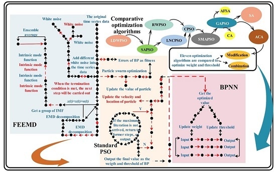
2. Time Series Decomposition

The preprocessing of the time series plays an important part in improving the forecasting accuracy by obtaining a smoother time series. The essence of empirical mode decomposition is the stabilization processing of a signal through decomposing the fluctuation or tendency in the real signal and then generating a series of data sequences with different characteristic scales. In recent years, this approach has gradually shown its unique advantages in processing non-stationary and non-linear signals [47]. However, it suffers from the mode mixing problem. As an improved algorithm, ensemble empirical mode decomposition overcomes this drawback of empirical mode decomposition and maintains the advantages, giving it wider applications [48]. The basic concept of ensemble empirical mode decomposition is to add Gaussian white noise to the analysed signal equally, and signal regions with different scales can map suitable scales in relation to the background white noise. Each single signal could generate very noisy results because each test has the white noise added. However, the added white noise would ultimately be eliminated because it has zero mean [49]. The overall average is regarded as the final results.

The detailed steps are as follows:

Step 1. Initialize the parameters. Set the number of integration ${\mathit{N}}_{\mathit{g}}$ according to the standard deviation of the signal, and the amplitude of added white noise is a. ${\mathit{N}}_{\mathit{g}}$ begins from 1 and $\mathit{m}\mathit{=}1$.

Step 2. Perform the process of decomposition using empirical mode decomposition. Decompose the added white noise signal and ${\mathit{x}}_{\mathit{m}}\mathit{=}\mathit{x}\mathit{+}{\mathit{n}}_{\mathit{m}}$: ${\mathit{n}}_{\mathit{m}}$ represents the added white noise with a pre-set amplitude, and x denotes the signal analysed. The decomposed results are called intrinsic mode functions (IMFs), denoted as ${\mathit{c}}_{\mathit{i}\mathit{,}\mathit{m}}\mathit{,}\mathit{(}\mathit{i}\mathit{=}1\mathit{,}2\mathit{,}\mathrm{...}\mathit{)}$. After decomposition, the remaining non-zero signal is the residual function ${\mathit{r}}_{\mathit{m}}$.

Step 3. Circle Step 2 through $\mathit{m}\mathit{=}\mathit{m}\mathit{+}1$ until the number of the integration arrives at ${\mathit{N}}_{\mathit{g}}$.

Step 4. Calculate the ensemble average of IMFs, obtaining the final result.

Remark 1. 

For each IMF or trend term, the kth white noise counteracts it after calculating the average. The IMF or trend term at each time maintains the natural dyadic filter window; therefore, the final average also maintains this type of quality, and the mixing mode problem is solved. Its pseudo-code is described below [38]. The pseudo-code of EEMD is described in Appendix A.

The ensemble empirical mode decomposition algorithm using parameters presented in [50] is termed the fast ensemble empirical mode decomposition, which can improve the efficiency of the algorithm. It would actually be applied to conduct the decomposition of each time series in this paper. Taking a short-term wind speed series for example, Figure 2 compares the data before and after noise reduction at three observation sites. The line chart shows that after reducing the noise, the time series data seems more stable, which can help to achieve higher forecasting accuracy. Moreover, the table shows that the standard deviation after the de-noising process is smaller than before the process.

3. Optimization of Back Propagation Neural Network

Due to the instability of the structure of back propagation, this section introduces optimization algorithms to optimize the weight and threshold of back propagation, including the standard particle swarm optimization algorithm and seven forms of improved particle swarm optimization algorithms.

3.1. Standard PSO Algorithm

PSO is an evolutionary algorithm classified in the swarm intelligence group based on bio-inspired algorithms, where a population of Np particles or the proposed solutions evolve with each iteration, moving towards the optimal solution of the problem [51]. In fact, a new population in the PSO algorithm is obtained by shifting the positions of the previous one in each iteration, and each individual would be affected by its neighbour’s trajectory and its own during its movement [51,52].

A standard PSO has certain features.

Feature 1. First, during the initial period, the solutions show stronger randomness with increasing iterations.

Feature 2. Second, one of the advantages of PSO is the application of real number coding, unlike the binary coding of the GA algorithm.

Feature 3. Third, particles can remember through learning from the last generation to find the best solution in the shortest time. Finally, compared with the GA algorithm, the information flow is unidirectional, which means that only ${\mathit{g}}_{\mathit{b}\mathit{e}\mathit{s}\mathit{t}}$ can deliver information to other particles. The basic steps of the standard PSO are as follows:

Step 1. Initialize the velocity and position of each particle in the population: ${\mathit{p}}_{\mathit{b}\mathit{e}\mathit{s}\mathit{t}}$ indicates the previous optimal position of each particle, and ${\mathit{g}}_{\mathit{b}\mathit{e}\mathit{s}\mathit{t}}$ represents the global optimal position.

Step 2. Calculate the objective function value, the fitness, of each particle.

Step 3. Update the velocity and position of each particle according to Equations (1) and (2).

$${\mathit{v}}_{\mathit{i}\mathit{.}\mathit{j}}\mathit{(}\mathit{t}\mathit{+}1\mathit{)}\mathit{=}\mathit{w}{\mathit{v}}_{\mathit{i}\mathit{.}\mathit{j}}\mathit{(}\mathit{t}\mathit{)}\mathit{+}{\mathit{c}}_1{\mathit{r}}_1\mathit{[}{\mathit{p}}_{\mathit{i}\mathit{.}\mathit{j}}\mathit{-}{\mathit{x}}_{\mathit{i}\mathit{.}\mathit{j}}\mathit{(}\mathit{t}\mathit{)}\mathit{]}\mathit{+}{\mathit{c}}_2{\mathit{r}}_2\mathit{[}{\mathit{p}}_{\mathit{g}\mathit{.}\mathit{j}}\mathit{-}{\mathit{x}}_{\mathit{i}\mathit{.}\mathit{j}}\mathit{(}\mathit{t}\mathit{)}\mathit{]}$$

(1)

$${\mathit{x}}_{\mathit{i}\mathit{.}\mathit{j}}\mathit{(}\mathit{t}\mathit{+}1\mathit{)}\mathit{=}{\mathit{x}}_{\mathit{i}\mathit{.}\mathit{j}}\mathit{(}\mathit{t}\mathit{)}\mathit{+}{\mathit{v}}_{\mathit{i}\mathit{.}\mathit{j}}\mathit{(}\mathit{t}\mathit{+}1\mathit{)}\mathit{,}\mathit{j}\mathit{=}1\mathit{,}\mathrm{...}\mathit{,}\mathit{d}$$

(2)

where w means the inertia weight, ${\mathit{c}}_1$ is a constant called the cognitive or local weight, and ${\mathit{c}}_2$ is a constant called the social or global weight.

Step 4. Calculate the fitness of each particle after the update, and ensure the new ${\mathit{p}}_{\mathit{b}\mathit{e}\mathit{s}\mathit{t}}$ and ${\mathit{g}}_{\mathit{b}\mathit{e}\mathit{s}\mathit{t}}$.

The pseudo-code of the standard PSO algorithm is listed in Appendix B.

3.2. Modified PSO Algorithm

This section introduces the modification of the PSO algorithm, including the inertia weight, constraint factor and learning factor. For the inertia weight, three types of modifications are introduced, which are the linear decreasing, self-adaptive and random inertia weight. The premise for the modification of each part of the PSO is that the other parts of the PSO remain unchanged.

3.2.1. Linear Decreasing Inertia Weight Particle Swarm Optimization (LDWPSO)

Definition 1. 

The inertia weight could influence both the local optimization and global optimization of particles. A larger inertia weight ${\mathit{w}}_{\mathbf{max}}$ is beneficial in improving the global searching ability; in comparison, a smaller inertia weight ${\mathit{w}}_{\mathbf{min}}$ could enhance the local searching ability of the algorithm. The transformation formula is as follows:

$$\mathit{w}\mathit{=}{\mathit{w}}_{\mathbf{max}}\mathit{-}\frac{\mathit{t}\mathit{\times }\mathit{(}{\mathit{w}}_{\mathbf{max}}\mathit{-}{\mathit{w}}_{\mathbf{min}}\mathit{)}}{{\mathit{t}}_{\mathbf{max}}}$$

(3)

where t is the number of iterations, and ${\mathit{t}}_{\mathbf{max}}$ is the maximum number of iterations.

Remark 2. 

According to Definition 1, we have modified the inertia weight based on Equation (3). The linear decreasing inertia weight can achieve a high global search ability.

3.2.2. Self-Adaptive Inertia Weight Particle Swarm Optimization (SAPSO)

Definition 2. 

The self-adaptive inertia weight w is conductive to balancing the local and global search ability and belongs to the non-linear adjustment method. When the fitness of each particle tends to be uniform or the local optimum, the inertia weight w increases. At the same time, if the fitness is better than the average fitness of each particle, the corresponding inertia weight is smaller, so this particle can stay. The adjustment equation is given below:

$$\mathit{w}\mathit{=}\mathit{\{}\begin{array}{l}{\mathit{w}}_{\mathbf{min}}\mathit{-}\frac{\mathit{(}{\mathit{w}}_{\mathbf{max}}\mathit{-}{\mathit{w}}_{\mathbf{min}}\mathit{)}\mathit{\times }\mathit{(}\mathit{f}\mathit{-}{\mathit{f}}_{\mathbf{min}}\mathit{)}}{{\mathit{f}}_{\mathit{a}\mathit{v}\mathit{g}}\mathit{-}{\mathit{f}}_{\mathbf{min}}}\mathit{,}\mathit{f}\mathit{\le }{\mathit{f}}_{\mathit{a}\mathit{v}\mathit{g}}\\ {\mathit{w}}_{\mathbf{max}}\mathit{,}\mathit{f}\mathit{>}{\mathit{f}}_{\mathit{a}\mathit{v}\mathit{g}}\end{array}$$

(4)

where ${\mathit{w}}_{\mathbf{max}}$ is the maximum inertia weight and ${\mathit{w}}_{\mathbf{min}}$ is the minimum inertia weight, ${\mathit{f}}_{\mathbf{min}}$ is the minimum fitness, ${\mathit{f}}_{\mathit{a}\mathit{v}\mathit{g}}$ is the average fitness, and f is the fitness.

Remark 3. 

According to Definition 2, we have modified the inertia weight based on Equation (4). The self-adaptive inertia weight has a higher ability to balance the local and global searching, which is beneficial to searching for the optimal particle.

3.2.3. Random Weight Particle Swarm Optimization (RWPSO)

The other way to overcome the shortcomings of the linearly decreasing inertia weight is to choose w randomly.

Definition 3. 

Random weight. If the best solution is obtained at the beginning of the evolution, the inertia weight w could be generated smaller at random, which it is helpful in accelerating the velocity of the particle. Furthermore, if the best solution cannot be found at the beginning, the random inertia weight w can overcome the disadvantage of the slow convergence rate. The change equation of the inertia weight is as follows:

$$\mathit{w}\mathit{=}0.5\mathit{+}\frac{\mathit{r}\mathit{a}\mathit{n}\mathit{d}\mathit{(}\mathit{)}}{2.0}$$

(5)

Remark 4. 

According to Definition 3, we can obtain a random w between 0.5 and 1. Such modification can bring the particle swarms closer to the objective function, which achieves a higher forecasting accuracy and convergence rate.

3.2.4. Constriction Factor Particle Swarm Optimization (CPSO)

Definition 4. 

Particles can control the flying speed effectively, allowing the algorithm to reach a balance of global and local exploration. The velocity equation is described below:

$${\mathit{v}}_{\mathit{i}\mathit{.}\mathit{j}}\mathit{=}\mathsf{\varphi }\mathit{\{}{\mathit{v}}_{\mathit{i}\mathit{.}\mathit{j}}\mathit{(}\mathit{t}\mathit{)}\mathit{+}{\mathit{c}}_1{\mathit{r}}_1\mathit{[}{\mathit{p}}_{\mathit{i}\mathit{.}\mathit{j}}\mathit{-}{\mathit{x}}_{\mathit{i}\mathit{.}\mathit{j}}\mathit{(}\mathit{t}\mathit{)}\mathit{]}\mathit{+}{\mathit{c}}_2{\mathit{r}}_2\mathit{[}{\mathit{p}}_{\mathit{g}\mathit{.}\mathit{j}}\mathit{-}{\mathit{x}}_{\mathit{i}\mathit{.}\mathit{j}}\mathit{(}\mathit{t}\mathit{)}\mathit{]}\mathit{\}}$$

(6)

where $\mathsf{\varphi }$ is the constriction factor, $\mathsf{\varphi }\mathit{=}\frac{2}{\mathit{\left|}2\mathit{-}\mathit{C}\mathit{-}\sqrt{{\mathit{C}}^2\mathit{-}4\mathit{C}}\mathit{\right|}}$, $\mathit{C}\mathit{=}{\mathit{c}}_1\mathit{+}{\mathit{c}}_2$ and C > 4.

Remark 5. 

According to Definition 4, we have modified the constriction factor based on Equation (6). The introduction of constriction factors is beneficial in ensuring the convergence of the particles and cancelling the constraint of the border on the velocity.

3.2.5. Learning Factor Change Particle Swarm Optimization (LNCPSO)

Definition 5. 

The experience information of each particle and its influences on the movement trail of the experience information of other particles are determined by the learning factor C, which reflects the exchange of information between particles. A larger ${\mathit{c}}_1$ would allow particles to wander in the local region, and a larger ${\mathit{c}}_2$ would result in the early convergence of a local optimum. The change equation is listed below:

$${\mathit{c}}_1\mathit{=}{\mathit{c}}_2\mathit{=}\frac{{\mathit{c}}_{\mathbf{max}}\mathit{-}{\mathit{c}}_{\mathbf{min}}}{{\mathit{t}}_{\mathbf{max}}}\mathit{\times }\mathit{t}\mathit{,}{\mathit{c}}_1\mathit{,}{\mathit{c}}_2\mathit{\in }\mathit{[}{\mathit{c}}_{\mathbf{min}}\mathit{,}{\mathit{c}}_{\mathbf{max}}\mathit{]}$$

(7)

where t represents the number of iterations, and ${\mathit{c}}_{\mathbf{max}}$ and ${\mathit{c}}_{\mathbf{min}}$ denote the maximum and minimum learning factor, respectively.

Remark 6. 

According to Definition 5, we have modified the learning factor of PSO based on Equation (7). The modification can achieve a balance between c₁ and c₂, which ensures a suitable convergence rate and searching ability.

3.3. Combination with Other Intelligent Algorithms

3.3.1. Combination with Simulated Annealing Algorithm (SMAPSO)

The simulated annealing algorithm could accept both a good solution and a bad solution with defined probabilities during the search process. At the same time, SA is effective for avoiding falling into a local optimum. The algorithm starts from a certain initial solution and then generates another solution from the neighbourhood randomly.

Step 1. Initialize the location m and velocity v of the particles according to random methods.

Step 2. Calculate the fitness of each particle based on the fitness function, and assign the fitness value of each particle to ${\mathit{P}}_{\mathit{i}}$.

Step 3. Implement the simulated annealing.

(a)

Set the initial temperature ${\mathit{T}}_{\mathit{k}}“\mathit{k}\mathit{=}0”$, and generate the initial solution ${\mathit{x}}_0$.

(b)

Repeat the following steps at temperature ${\mathit{T}}_{\mathit{k}}$ until ${\mathit{T}}_{\mathit{k}}$ arrives at a balanced state.

Generate a new solution ${\mathit{x}}^{\mathit{\prime }}$ in the domain of x; calculate the objective function $\mathit{f}\mathit{(}{\mathit{x}}^{\mathit{\prime }}\mathit{)}$ of ${\mathit{x}}^{\mathit{\prime }}$ and the objective function $\mathit{f}\mathit{(}\mathit{x}\mathit{)}$ of x; calculate the difference between $\mathit{f}\mathit{(}{\mathit{x}}^{\mathit{\prime }}\mathit{)}$ and $\mathit{f}\mathit{(}\mathit{x}\mathit{)}$; and obtain ${\mathit{x}}^{\mathit{\prime }}$ according to $\mathbf{min}\mathit{\{}1\mathit{,}\mathit{exp}\mathit{(}\mathit{-}\mathbf{\Delta }\mathit{f}\mathit{/}{\mathit{T}}_{\mathit{k}}\mathit{)}\mathit{\}}\mathit{>}\mathit{r}\mathit{a}\mathit{n}\mathit{d}\mathit{o}\mathit{m}\mathit{[}0\mathit{,}1\mathit{]}$.

(c)

Annealing. ${\mathit{T}}_{\mathit{k}\mathit{+}1}\mathit{=}\mathit{C}{\mathit{T}}_{\mathit{k}\mathit{,}}\mathit{k}\mathit{\leftarrow }\mathit{k}\mathit{+}1$; if the condition of convergence is met, then the annealing process ends. Otherwise, return to (b).

Step 4. Calculate the fitness value of each particle at the current temperature, using the equation shown below:

$$\mathit{T}\mathit{F}\mathit{(}{\mathit{P}}_{\mathit{i}}\mathit{)}\mathit{=}\frac{{\mathit{e}}^{\mathit{-}\mathit{(}\mathit{f}\mathit{(}{\mathit{P}}_{\mathit{i}}\mathit{)}\mathit{-}\mathit{f}\mathit{(}{\mathit{P}}_{\mathit{g}}\mathit{)}\mathit{)}\mathit{/}\mathit{t}}}{{\displaystyle \mathit{\sum }_{\mathit{i}\mathit{=}1}^{\mathit{N}}{\mathit{e}}^{\mathit{-}\mathit{(}\mathit{f}\mathit{(}{\mathit{P}}_{\mathit{i}}\mathit{)}\mathit{-}\mathit{f}\mathit{(}{\mathit{P}}_{\mathit{g}}\mathit{)}\mathit{)}\mathit{/}\mathit{t}}}}$$

(8)

Step 5. Update the location and velocity of each particle, ensure the global optimal value ${{\mathit{P}}^{\mathit{\prime }}}_{\mathit{g}}$, and calculate the new fitness.

3.3.2. Combination with Genetic Algorithm (GAPSO)

The genetic algorithm (GA) conducts a search based on the population of chromosomes with the operations of selection, crossover and mutation. GA has the ability to update particles rapidly, avoiding the premature convergence problem of standard particle swarm optimization. Therefore, the advantages of GAs can compensate perfectly for the disadvantages of particle swarm optimization [52].

Step 1. Initialize the number of particles m of group U, and set the maximum iteration to N.

Step 2. Calculate the fitness according to Equation (9).

$$\mathit{F}\mathit{i}\mathit{t}\mathit{n}\mathit{e}\mathit{s}\mathit{s}\mathit{=}\frac{\mathit{k}}{{\displaystyle \mathit{\sum }_{\mathit{i}\mathit{=}1}^{\mathit{k}}{\mathit{(}{\mathit{t}}_{\mathit{i}}\mathit{-}{\mathit{y}}_{\mathit{i}}\mathit{)}}^2}}\mathit{+}\mathit{b}$$

(9)

where Fitness is the fitness function, and k and b are both constants. Here, ${\mathit{t}}_{\mathit{i}}$ is the actual value, and ${\mathit{y}}_{\mathit{i}}$ is the forecasted value.

Step 3. Introduce the selection, crossover and mutation of the genetic algorithm. The group with the better fitness is selected for the next generation. Then, the crossover operation of the location and speed between i and j is given below:

$$\mathit{\{}\begin{array}{l}{\mathit{v}}_{\mathit{i}}\mathit{(}\mathit{t}\mathit{+}1\mathit{)}\mathit{=}{\mathsf{\theta }}_1\mathit{\times }{\mathit{v}}_{\mathit{i}}\mathit{(}\mathit{t}\mathit{)}\mathit{+}\mathit{(}1\mathit{-}{\mathsf{\theta }}_1\mathit{)}\mathit{\times }{\mathit{v}}_{\mathit{j}}\mathit{(}\mathit{t}\mathit{)}\\ {\mathit{v}}_{\mathit{j}}\mathit{(}\mathit{t}\mathit{+}1\mathit{)}\mathit{=}\mathit{(}1\mathit{-}{\mathsf{\theta }}_1\mathit{)}\mathit{\times }{\mathit{v}}_{\mathit{i}}\mathit{(}\mathit{t}\mathit{)}\mathit{+}{\mathsf{\theta }}_1\mathit{\times }{\mathit{v}}_{\mathit{j}}\mathit{(}\mathit{t}\mathit{)}\end{array}$$

(10)

$$\mathit{\{}\begin{array}{l}{\mathit{x}}_{\mathit{i}}\mathit{(}\mathit{t}\mathit{+}1\mathit{)}\mathit{=}{\mathsf{\theta }}_2\mathit{\times }{\mathit{x}}_{\mathit{i}}\mathit{(}\mathit{t}\mathit{)}\mathit{+}\mathit{(}1\mathit{-}{\mathsf{\theta }}_2\mathit{)}\mathit{\times }{\mathit{x}}_{\mathit{j}}\mathit{(}\mathit{t}\mathit{)}\\ {\mathit{x}}_{\mathit{j}}\mathit{(}\mathit{t}\mathit{+}1\mathit{)}\mathit{=}\mathit{(}1\mathit{-}{\mathsf{\theta }}_2\mathit{)}\mathit{\times }{\mathit{x}}_{\mathit{i}}\mathit{(}\mathit{t}\mathit{)}\mathit{+}{\mathsf{\theta }}_2\mathit{\times }{\mathit{x}}_{\mathit{j}}\mathit{(}\mathit{t}\mathit{)}\end{array}$$

(11)

Step 4. Update the individual optimum and global optimum of the groups. Compare the current fitness of each particle and the fitness of the individual optimum pbest. If the current fitness is better, then update pbest. Compare the individual optimum pbest and the global optimum of the group gbest. If the current pbest is better than gbest, then update gbest.

Step 5. Repeat the above steps until the iteration reaches its maximum value.

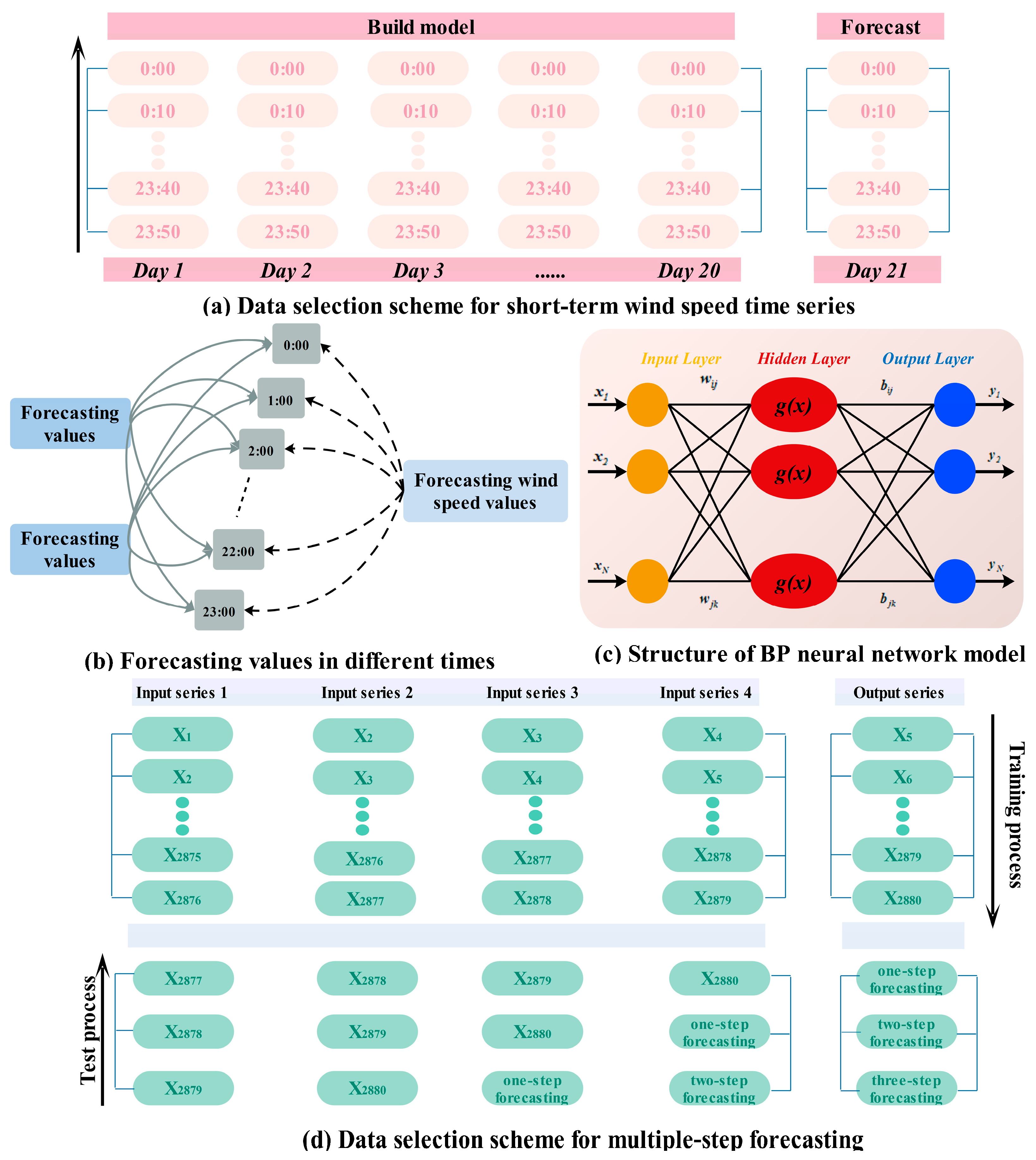
3.4. Back Propagation Neural Network

A back propagation neural network is a feed-forward neural network implemented by the back propagation algorithm and it is among the most widely applied neural network modes [53]. Back propagation can learn and store a large amount of input-output map relations without revealing the mathematical equation that describes the relation. The learning rule is the steepest descent method, and the sum of squared errors is minimized through the back propagation continuously adjusting the weight and threshold [54].

Definition 6. 

The weight and threshold are two important network parameters, and their adjustment formula can be expressed as follows:

$${\mathit{w}}_{\mathit{k}\mathit{j}}\mathit{(}\mathit{t}\mathit{+}1\mathit{)}\mathit{=}{\mathit{w}}_{\mathit{k}\mathit{j}}\mathit{(}\mathit{t}\mathit{)}\mathit{+}\mathsf{\alpha }{\mathsf{\delta }}_{\mathit{k}}{\mathit{H}}_{\mathit{j}}$$

(12)

$${\mathit{u}}_{\mathit{j}\mathit{h}}\mathit{(}\mathit{t}\mathit{+}1\mathit{)}\mathit{=}{\mathit{u}}_{\mathit{j}\mathit{h}}\mathit{(}\mathit{t}\mathit{)}\mathit{+}\mathsf{\alpha }{\mathsf{\sigma }}_{\mathit{j}}{\mathit{I}}_{\mathit{h}}$$

(13)

$${\mathsf{\theta }}_{\mathit{k}}\mathit{(}\mathit{t}\mathit{+}1\mathit{)}\mathit{=}{\mathsf{\theta }}_{\mathit{k}}\mathit{(}\mathit{t}\mathit{)}\mathit{+}\mathsf{\beta }{\mathsf{\delta }}_{\mathit{k}}$$

(14)

$${\widehat{\mathsf{\theta }}}_{\mathit{j}}\mathit{(}\mathit{t}\mathit{+}1\mathit{)}\mathit{=}{\widehat{\mathsf{\theta }}}_{\mathit{j}}\mathit{(}\mathit{t}\mathit{)}\mathit{+}\mathsf{\beta }{\mathsf{\sigma }}_{\mathit{j}}$$

(15)

where ${\mathit{H}}_{\mathit{j}}$ is the output of hidden node j; ${\mathit{I}}_{\mathit{h}}$ is the input signal from input node h; ${\mathit{w}}_{\mathit{k}\mathit{j}}\mathit{(}\mathit{t}\mathit{)}$ and ${\mathit{w}}_{\mathit{k}\mathit{j}}\mathit{(}\mathit{t}\mathit{+}1\mathit{)}$ are the weights between hidden node j and output node k before and after the training; ${\mathit{u}}_{\mathit{j}\mathit{h}}\mathit{(}\mathit{t}\mathit{)}$ and ${\mathit{u}}_{\mathit{j}\mathit{h}}\mathit{(}\mathit{t}\mathit{+}1\mathit{)}$ are the weights between hidden node j and input node h before and after the training; ${\mathsf{\theta }}_{\mathit{k}}$ and ${\widehat{\mathsf{\theta }}}_{\mathit{j}}$ are separately the threshold of output node k and hidden node j; $\mathsf{\alpha }$ and $\mathsf{\beta }$ are the learning parameters between 0.1 and 0.9; and ${\mathsf{\delta }}_{\mathit{k}}$ and ${\mathsf{\sigma }}_{\mathit{j}}$ are the error signals of output node k and hidden node j, with the following equations:

$${\mathsf{\delta }}_{\mathit{k}}\mathit{=}\mathit{(}{\mathit{T}}_{\mathit{k}}\mathit{-}{\mathit{O}}_{\mathit{k}}\mathit{)}{\mathit{O}}_{\mathit{k}}\mathit{(}1\mathit{-}{\mathit{O}}_{\mathit{k}}\mathit{)}$$

(16)

$${\mathsf{\sigma }}_{\mathit{j}}\mathit{=}{\displaystyle \mathit{\sum }_{\mathit{k}}{\mathsf{\delta }}_{\mathit{k}}{\mathit{w}}_{\mathit{k}\mathit{j}}{\mathit{H}}_{\mathit{j}}\mathit{(}1\mathit{-}{\mathit{H}}_{\mathit{j}}\mathit{)}}$$

(17)

where ${\mathit{T}}_{\mathit{k}}$ is the target output for output node k. ${\mathit{O}}_{\mathit{k}}$ and ${\mathit{H}}_{\mathit{j}}$ are the actual output in output node k and hidden node j. The formula of ${\mathit{H}}_{\mathit{j}}$ is given below:

$${\mathit{H}}_{\mathit{i}}\mathit{=}\mathit{f}\mathit{[}{\displaystyle \mathit{\sum }_{\mathit{h}\mathit{=}1}^{{\mathit{n}}_{\mathit{i}}}{\mathit{u}}_{\mathit{j}\mathit{h}}{\mathit{I}}_{\mathit{h}}\mathit{+}{\widehat{\mathsf{\theta }}}_{\mathit{j}}}\mathit{]}$$

(18)

where ${\mathit{n}}_{\mathit{i}}$ is the number of input nodes. The function f is the S activation function:

$$\mathit{f}\mathit{(}\mathit{x}\mathit{)}\mathit{=}\frac{1}{1\mathit{+}{\mathit{e}}^{\mathit{-}\mathit{x}}}$$

(19)

The output layer calculates the sum using a linear weighting method:

$${\mathit{O}}_{\mathit{k}}\mathit{=}{\displaystyle \mathit{\sum }_{\mathit{j}\mathit{=}1}^{{\mathit{n}}_{\mathit{h}}}{\mathit{w}}_{\mathit{k}\mathit{j}}{\mathit{H}}_{\mathit{j}}\mathit{+}{\mathsf{\theta }}_{\mathit{k}}}$$

(20)

where ${\mathit{n}}_{\mathit{h}}$ is the number of hidden nodes.

3.5. The Hybrid Models

The time series data in the electrical system exhibit high fluctuation, so it is necessary to denoise the time series data in advance. The fast ensemble empirical mode decomposition introduced above is applied for the decomposition of the data to improve the forecasting accuracy. Artificial neural networks can obtain the data laws and can be used in time series forecasting. Among them, the back propagation neural network is one of the most widely applied neural network modes. However, in practical application, it still has some limitations. It is difficult to determine the weight and threshold of the structure of back propagation. Accordingly, seven improved particle swarm optimization algorithms were all employed to seek the optimal value of the weight and threshold of back propagation and compared to determine the most effective hybrid model for time series forecasting. The detailed steps are listed below and shown in Figure 3.

Step 1. Fast ensemble empirical mode decomposition is employed to denoise the original time series data of three indicators.

$$\mathit{s}\mathit{(}\mathit{t}\mathit{)}\mathit{=}{\displaystyle \mathit{\sum }_{\mathit{j}\mathit{=}1}^{\mathit{n}}{\mathit{c}}_{\mathit{j}}\mathit{(}\mathit{t}\mathit{)}\mathit{+}{\mathit{r}}_{\mathit{n}}\mathit{(}\mathit{t}\mathit{)}}$$

(21)

Step 2. Back propagation is introduced to forecast the time series data of wind speed, electricity price, and electrical load.

Step 3. The seven improved particle swarm optimization algorithms are applied to optimize the weight and threshold of the structure of back propagation. The loss function and weight allocation are listed below:

$$\mathit{y}\mathit{=}\mathit{m}\mathit{e}\mathit{a}\mathit{n}{\mathit{(}{\widehat{\mathit{x}}}_{\mathit{s}}^{\mathit{(}0\mathit{)}}\mathit{-}{\mathit{x}}_{\mathit{s}}^{\mathit{(}0\mathit{)}}\mathit{)}}^2$$

(22)

$$\mathit{\{}\begin{array}{l}{\mathit{w}}_{\mathit{k}\mathit{j}}\mathit{=}\mathit{x}\mathit{(}1\mathit{:}\mathit{w}1\mathit{r}\mathit{\times }\mathit{w}1\mathit{c}\mathit{)}\\ {\mathit{u}}_{\mathit{j}\mathit{h}}\mathit{=}\mathit{x}\mathit{(}1\mathit{+}\mathit{w}1\mathit{r}\mathit{\times }\mathit{w}1\mathit{c}\mathit{:}\mathit{w}1\mathit{r}\mathit{\times }\mathit{w}1\mathit{c}\mathit{+}\mathit{w}2\mathit{r}\mathit{\times }\mathit{w}2\mathit{c}\mathit{)}\\ {\mathsf{\theta }}_{\mathit{k}}\mathit{=}\mathit{x}\mathit{(}1\mathit{+}\mathit{w}1\mathit{r}\mathit{\times }\mathit{w}1\mathit{c}\mathit{+}\mathit{w}2\mathit{r}\mathit{\times }\mathit{w}2\mathit{c}\mathit{:}\mathit{w}1\mathit{r}\mathit{\times }\mathit{w}1\mathit{c}\mathit{+}\mathit{w}2\mathit{r}\mathit{\times }\mathit{w}2\mathit{c}\mathit{+}\mathit{b}1\mathit{r}\mathit{\times }\mathit{b}1\mathit{c}\mathit{)}\\ {\widehat{\mathsf{\theta }}}_{\mathit{j}}\mathit{=}\mathit{x}\mathit{(}\mathit{w}1\mathit{r}\mathit{\times }\mathit{w}1\mathit{c}\mathit{+}\mathit{w}2\mathit{r}\mathit{\times }\mathit{w}2\mathit{c}\mathit{+}\mathit{b}1\mathit{r}\mathit{\times }\mathit{b}1\mathit{c}\mathit{:}\mathit{w}1\mathit{r}\mathit{\times }\mathit{w}1\mathit{c}\mathit{+}\mathit{w}2\mathit{r}\mathit{\times }\mathit{w}2\mathit{c}\mathit{+}\mathit{b}1\mathit{r}\mathit{\times }\mathit{b}1\mathit{c}\mathit{+}\mathit{b}2\mathit{r}\mathit{\times }\mathit{b}2\mathit{c}\mathit{)}\end{array}$$

(23)

where w₁, w₂, b₁ and b₂ are the weight and threshold values, respectively.

Step 4. Four metrics, including MAPE, MAE, MSE and FVD, are used to evaluate the forecasting performance of the proposed hybrid models by comparing them with a series of traditional models, models combined with other algorithms and the single models.

Step 5. The hybrid models proposed in this paper forecast time series based on the historical data, and multi-step forecasting is conducted to testify further to the effectiveness of the model.

(a)

One-step forecasting: The forecasted value $\widehat{\mathit{x}}\mathit{(}\mathit{t}\mathit{+}1\mathit{)}$ is obtained based on the historical time series $\mathit{\{}\mathit{x}\mathit{(}1\mathit{)}\mathit{,}\mathit{x}\mathit{(}2\mathit{)}\mathit{,}\mathit{x}\mathit{(}3\mathit{)}\mathit{,}\mathrm{...}\mathit{,}\mathit{x}\mathit{(}\mathit{t}\mathit{-}1\mathit{)}\mathit{,}\mathit{x}\mathit{(}\mathit{t}\mathit{)}\mathit{\}}$, and t is the sampled time of the time series.

(b)

Two-step forecasting: The forecasted value $\widehat{\mathit{x}}\mathit{(}\mathit{t}\mathit{+}2\mathit{)}$ is obtained based on the historical time series $\mathit{\{}\mathit{x}\mathit{(}1\mathit{)}\mathit{,}\mathit{x}\mathit{(}2\mathit{)}\mathit{,}\mathit{x}\mathit{(}3\mathit{)}\mathit{,}\mathrm{...}\mathit{,}\mathit{x}\mathit{(}\mathit{t}\mathit{-}1\mathit{)}\mathit{,}\mathit{x}\mathit{(}\mathit{t}\mathit{)}\mathit{\}}$ and the previously forecasted value $\widehat{\mathit{x}}\mathit{(}\mathit{t}\mathit{+}1\mathit{)}$.

(c)

Three-step forecasting: The forecasted value $\widehat{\mathit{x}}\mathit{(}\mathit{t}\mathit{+}3\mathit{)}$ is calculated based on the historical time series $\mathit{\{}\mathit{x}\mathit{(}1\mathit{)}\mathit{,}\mathit{x}\mathit{(}2\mathit{)}\mathit{,}\mathit{x}\mathit{(}3\mathit{)}\mathit{,}\mathrm{...}\mathit{,}\mathit{x}\mathit{(}\mathit{t}\mathit{-}1\mathit{)}\mathit{,}\mathit{x}\mathit{(}\mathit{t}\mathit{)}\mathit{\}}$ and the previously forecasted values $\mathit{\{}\widehat{\mathit{x}}\mathit{(}\mathit{t}\mathit{+}1\mathit{)}\mathit{,}\widehat{\mathit{x}}\mathit{(}\mathit{t}\mathit{+}2\mathit{)}\mathit{\}}$.

Figure 3 presents the flow chart of the hybrid models. The first part of the hybrid model is the FEEMD. White noise is added to the original time series data, and EMD decomposition is conducted to obtain the intrinsic mode functions. The preprocessed time series data are used to forecast the wind speed, electrical load and electricity price. The second part is BPNN optimized by different types of PSO, including LDWPSO, RWPSO, SAPSO, LNCPSO, CPSO, SMAPSO and GAPSO. Through optimizing and updating the weight and threshold values in BP, the optimal values can be obtained for forecasting.

4. Experimental Simulation and Results Analysis

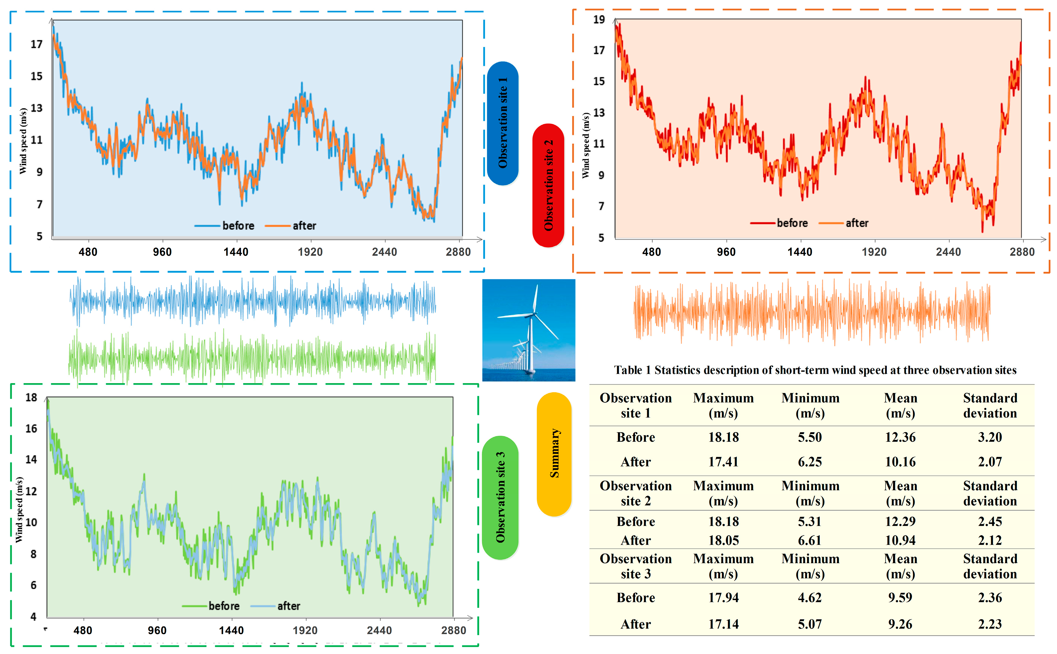
This section is aimed at proving the effectiveness of the proposed hybrid models through four experiments after introducing the data sets, data preprocessing and evaluation metrics. The four experiments compare the hybrid models with other famous traditional forecasting models, models with different optimization algorithms and forecasting with different steps.

4.1. Data Sets

This paper selects three indicators for forecasting in the electrical system: the data sets include a short-term wind speed time series, an electrical load time series and an electricity price time series. First, for short-term wind speed data, the time interval is 10 min, covering from 1 January to 25 January at three observation sites. The data from 20 days are applied to forecast the data for one day. The number of training data points is 2880, and the number of testing data points is 144. For example, the first training data set covers from 1 January to 20 January, and the corresponding testing data set is 21 January. Similarly, the final training data set is from 5 January to 24 January, and the corresponding testing data set is 25 January. The average of five forecasting days would be calculated as the final results of the hybrid model at each observation site to overcome the instability of back propagation. For the electrical load and electricity price time series data sets, the span is from 1 January to 25 January, collected from New South Wales (NSW). The data from 20 days are used to forecast the data for one day. The number of training data points is 960, and the number of testing data points is 48. The data applied in this paper are all primary data obtained from the local wind farms.

Figure 4 describes the data selection scheme of three indicators in the electrical power system. Figure 4a shows how to choose the data to build the model and conduct the forecasting. Figure 4b shows the forecasting values of the time series data. Figure 4c is the structure of the BPNN, including the input, hidden and output layers. Finally, Figure 4d depicts the data selection scheme for multiple-step forecasting.

4.2. Evaluation Metrics

It is crucial to apply effective evaluation metrics to assess the forecasting accuracy and this paper introduces two types of metrics: the evaluation of multiple points and the overall performance of the model.

4.2.1. Evaluation of Multiple Points

In addition to evaluating a single point, it is also necessary to assess the forecasting accuracy of multiple points. Three metrics, including MAE, RMSE and MAPE, are applied for this evaluation.

MAE and RMSE measure the average magnitude of the forecasting errors, and their equations are given below:

$$\mathit{M}\mathit{A}\mathit{E}\mathit{=}\frac{1}{\mathit{n}}{\displaystyle \mathit{\sum }_{\mathit{i}\mathit{=}1}^{\mathit{n}}\mathit{\left|}{\mathit{x}}_{\mathit{(}0\mathit{)}}\mathit{(}\mathit{t}\mathit{)}\mathit{-}{\widehat{\mathit{x}}}_{\mathit{(}0\mathit{)}}\mathit{(}\mathit{t}\mathit{)}\mathit{\right|}}$$

(24)

$$\mathit{M}\mathit{S}\mathit{E}\mathit{=}\frac{1}{\mathit{n}}{{\displaystyle {\mathit{\sum }}_{\mathit{i}\mathit{=}1}^{\mathit{n}}\mathit{\left|}{\mathit{x}}_{\mathit{(}0\mathit{)}}\mathit{(}\mathit{t}\mathit{)}\mathit{-}{\widehat{\mathit{x}}}_{\mathit{(}0\mathit{)}}\mathit{(}\mathit{t}\mathit{)}\mathit{\right|}}}^2$$

(25)

MAPE is an effective method for measuring forecasting errors, and smaller values indicate a higher degree of forecasting accuracy of the model. The MAPE criteria are listed in

Table 2. Criterion of MAPE.

MAPE(%)	Forecasting Degree
<10	Excellent
10–20	Good
20–50	Reasonable
>50	Incorrect

[55]. If the value of MAPE is smaller than 10%, the forecasting degree is excellent; if the value is between 10% and 20%, the forecasting degree is good; if the value is between 20% and 50%, the forecasting degree is reasonable; however, if the value is larger than 50%, the forecasting degree is incorrect, which indicates that the forecasting result is very poor.

$$\mathit{M}\mathit{A}\mathit{P}\mathit{E}\mathit{(}\mathit{\%}\mathit{)}\mathit{=}\frac{1}{\mathit{n}}{\displaystyle {\mathit{\sum }}_{\mathit{i}\mathit{=}1}^{\mathit{n}}\mathit{\left|}\frac{{\mathit{x}}_{\mathit{(}0\mathit{)}}\mathit{(}\mathit{t}\mathit{)}\mathit{-}{\widehat{\mathit{x}}}_{\mathit{(}0\mathit{)}}\mathit{(}\mathit{t}\mathit{)}}{{\mathit{x}}_{\mathit{(}0\mathit{)}}\mathit{(}\mathit{t}\mathit{)}}\mathit{\right|}}$$

(26)

4.2.2. Forecasting Validity Degree

Currently, the evaluation of the validity of most models uses the error sum of squares and the sum of the absolute value of the errors; in fact, these metrics cannot reflect the validity of forecasting methods well due to the different dimensions of different sequences. This paper introduces the forecasting validity degree based on the element of the invalid degree of k-order forecasting relative error [56]. The validity of forecasting methods should be reflected by the comprehensive and average accuracy. That is to say, a method with a high forecasting accuracy in certain periods may not have a high forecasting validity. When the forecasting accuracy is high in all periods, we can say that the method achieves a high forecasting validity. The greater the average forecasting accuracy, the higher the forecasting validity.

Assume the observed value of the indicator sequence is $\mathit{\{}{\mathit{x}}_{\mathit{t}}\mathit{,}\mathit{t}\mathit{=}1\mathit{,}2\mathit{,}\mathrm{...}\mathit{,}\mathit{N}\mathit{\}}$, there are m single forecasting methods to forecast the sequence, and ${\mathit{x}}_{\mathit{i}\mathit{t}}$ is the forecasting value at time t with the ith method, $\mathit{i}\mathit{=}1\mathit{,}2\mathit{,}\mathrm{...}\mathit{,}\mathit{m}\mathit{,}\mathit{t}\mathit{=}1\mathit{,}2\mathit{,}\mathrm{...}\mathit{,}\mathit{N}$. Some concepts are listed below

Definition 7. 

The value of ${\mathit{e}}_{\mathit{i}\mathit{t}}$ is the relative error of the ith method at time t ($\mathit{i}\mathit{=}1\mathit{,}2\mathit{,}\mathrm{...}\mathit{,}\mathit{m}\mathit{,}\mathit{t}\mathit{=}1\mathit{,}2\mathit{,}\mathrm{...}\mathit{,}\mathit{N}$). $\mathit{E}\mathit{=}{\mathit{(}{\mathit{e}}_{\mathit{i}\mathit{t}}\mathit{)}}_{\mathit{m}\mathit{\times }\mathit{N}}$ is the matrix of relative error.

$${\mathit{e}}_{\mathit{i}\mathit{t}}\mathit{=}\mathit{\{}\begin{array}{l}\mathit{-}1\mathit{,}\frac{{\mathit{x}}_{\mathit{t}}\mathit{-}{\mathit{x}}_{\mathit{i}\mathit{t}}}{{\mathit{x}}_{\mathit{t}}}\mathit{<}\mathit{-}1\\ \frac{{\mathit{x}}_{\mathit{t}}\mathit{-}{\mathit{x}}_{\mathit{i}\mathit{t}}}{{\mathit{x}}_{\mathit{t}}}\mathit{,}\mathit{-}1\mathit{<}\frac{{\mathit{x}}_{\mathit{t}}\mathit{-}{\mathit{x}}_{\mathit{i}\mathit{t}}}{{\mathit{x}}_{\mathit{t}}}\mathit{<}1\\ 1\mathit{,}\frac{{\mathit{x}}_{\mathit{t}}\mathit{-}{\mathit{x}}_{\mathit{i}\mathit{t}}}{{\mathit{x}}_{\mathit{t}}}\mathit{>}1\end{array}$$

(27)

Remark 7. 

Obviously, $0\mathit{\le }\mathit{\left|}{\mathit{e}}_{\mathit{i}\mathit{t}}\mathit{\right|}\mathit{\le }1$. Matrix E is the sequence of the forecasting relative error using the ith forecasting method at each time t. The tth column of E is the sequence of the forecasting relative error at time t with each method.

Definition 8. 

The forecasting accuracy of the ith method at time t is ${\mathit{A}}_{\mathit{i}\mathit{t}}\mathit{=}1\mathit{-}\mathit{\left|}{\mathit{e}}_{\mathit{i}\mathit{t}}\mathit{\right|}$ ($\mathit{i}\mathit{=}1\mathit{,}2\mathit{,}\mathrm{...}\mathit{,}\mathit{m}\mathit{,}\mathit{t}\mathit{=}1\mathit{,}2\mathit{,}\mathrm{...}\mathit{,}\mathit{N}$). Clearly, $0\mathit{\le }{\mathit{A}}_{\mathit{i}\mathit{t}}\mathit{\le }1$, and when $\mathit{\left|}\mathit{\left(}{\mathit{x}}_{\mathit{t}}\mathit{-}{\mathit{x}}_{\mathit{i}\mathit{t}}\mathit{\right)}\mathit{/}{\mathit{x}}_{\mathit{t}}\mathit{\right|}\mathit{>}1$, the forecasting accuracy is ${\mathit{A}}_{\mathit{i}\mathit{t}}\mathit{=}0$.

Remark 8. 

The value ${\mathit{e}}_{\mathit{i}\mathit{t}}$ has randomness due to the influences of all types of factors, so $\mathit{\left\{}{\mathit{A}}_{\mathit{i}\mathit{t}}\mathit{,}\mathit{i}\mathit{=}1\mathit{,}2\mathit{,}\mathit{\cdots }\mathit{,}\mathit{m}\mathit{,}\mathit{t}\mathit{=}1\mathit{,}2\mathit{,}\mathit{\cdots }\mathit{N}\mathit{\right\}}$ can be regarded as a sequence of random variables.

Definition 9. 

The element of the k-order forecasting validity degree with the ith method can be shown as follows:

$${\mathit{m}}_{\mathit{i}}^{\mathit{k}}\mathit{=}{\displaystyle \mathit{\sum }_{\mathit{t}\mathit{=}1}^{\mathit{N}}{\mathit{Q}}_{\mathit{t}}{\mathit{A}}_{\mathit{i}\mathit{t}}^{\mathit{k}}}$$

(28)

where k is the positive integer, $\mathit{\left(}\mathit{i}\mathit{=}1\mathit{,}2\mathit{,}\mathit{\cdots }\mathit{m}\mathit{\right)}$ and $\mathit{\left\{}{\mathit{Q}}_{\mathit{t}}\mathit{,}\mathit{t}\mathit{=}1\mathit{,}2\mathit{,}\mathit{\cdots }\mathit{,}\mathit{N}\mathit{\right\}}$ is the discrete probability distribution of the mth forecasting method at time t: ${\displaystyle \mathit{\sum }_{\mathit{t}\mathit{=}1}^{\mathit{N}}{\mathit{Q}}_{\mathit{t}}\mathit{=}1}\mathit{,}\mathit{\left(}{\mathit{Q}}_{\mathit{t}}\mathit{>}0\mathit{\right)}$.

Remark 9. 

When the a priori information of the discrete probability distribution is unknown, ${\displaystyle \mathit{\sum }_{\mathit{t}\mathit{=}1}^{\mathit{N}}{\mathit{Q}}_{\mathit{t}}\mathit{=}1}\mathit{/}\mathit{N}\mathit{,}\mathit{t}\mathit{=}1\mathit{,}2\mathit{,}\mathrm{...}\mathit{,}\mathit{N}$. In effect, ${\mathit{m}}_{\mathit{i}}^{\mathit{k}}$ is the k-order origin moment of the forecasting accuracy sequence $\mathit{\{}{\mathit{A}}_{\mathit{i}\mathit{t}}\mathit{,}\mathit{t}\mathit{=}1\mathit{,}2\mathit{,}\mathrm{...}\mathit{,}\mathit{N}\mathit{\}}$ with the ith forecasting method.

Definition 10. 

The k-order forecasting validity degree can be denoted as $\mathit{H}\mathit{\left(}{\mathit{m}}_{\mathit{i}}^1\mathit{,}{\mathit{m}}_{\mathit{i}}^2\mathit{,}\mathit{\cdots }\mathit{,}{\mathit{m}}_{\mathit{i}}^{\mathit{k}}\mathit{\right)}$, and H is a k-element continuous function.

Definition 11. 

When $\mathit{H}\mathit{\left(}\mathit{x}\mathit{\right)}\mathit{=}\mathit{x}$ is a one-element continuous function, $\mathit{H}\mathit{\left(}{\mathit{m}}_{\mathit{i}}^1\mathit{\right)}\mathit{=}{\mathit{m}}_{\mathit{i}}^1$ is the one-order forecasting validity of the ith forecasting method; when $\mathit{H}\mathit{\left(}{\mathit{x}}_{\mathit{i}}\mathit{\right)}\mathit{=}{\mathit{x}}_{\mathit{i}}\mathit{\left(}1\mathit{-}\sqrt{\mathit{y}\mathit{-}{\mathit{x}}_{\mathit{i}}^2}\mathit{\right)}$ is a two-element continuous function, $\mathit{H}\mathit{\left(}{\mathit{m}}_{\mathit{i}}^1\mathit{,}{\mathit{m}}_{\mathit{i}}^2\mathit{\right)}\mathit{=}{\mathit{m}}_{\mathit{i}}^1\mathit{\left(}1\mathit{-}\sqrt{{\mathit{m}}_{\mathit{i}}^2\mathit{-}{\mathit{\left(}{\mathit{m}}_{\mathit{i}}^1\mathit{\right)}}^2}\mathit{\right)}$ is the two-order forecasting validity of the ${\mathit{i}}_{\mathit{t}\mathit{h}}$ forecasting method.

Remark 10. 

Definition 11 indicates that the one-order forecasting validity index is the mathematical expectation of the forecasting accuracy series. When the difference between one and the standard deviation of the forecasting accuracy series is multiplied by its mathematical expectation, the two-order forecasting validity index is obtained [57].

According to Definition 7, we define the forecasting accuracy of the ith forecasting method at time t, ${\mathit{A}}_{\mathit{i}\mathit{t}}$, as follows:

$${\mathit{A}}_{\mathit{i}\mathit{t}}\mathit{=}\mathit{\{}\begin{array}{l}1\mathit{-}\mathit{\left|}{\mathit{e}}_{\mathit{i}\mathit{t}}\mathit{\right|}\mathit{,}0\mathit{\le }\mathit{\left|}{\mathit{e}}_{\mathit{i}\mathit{t}}\mathit{\right|}\mathit{\le }1\\ 0\mathit{,}\mathit{\left|}{\mathit{e}}_{\mathit{i}\mathit{t}}\mathit{\right|}\mathit{\ge }1\end{array}$$

(29)

It is clear that ${\mathit{A}}_{\mathit{i}\mathit{t}}$ has the property of a random variable.

Definition 12. 

The forecasting validity degree of the ith method in the forecasting interval (N + 1, N + T) can be expressed as

$${\mathit{m}}_{\mathit{i}\mathit{f}}\mathit{=}{\displaystyle \mathit{\sum }_{\mathit{t}\mathit{=}\mathit{N}\mathit{+}1}^{\mathit{N}\mathit{+}\mathit{T}}{\mathit{Q}}_{\mathit{i}\mathit{t}}{\mathit{A}}_{\mathit{i}\mathit{t}}}$$

(30)

where ${\mathit{Q}}_{\mathit{i}\mathit{t}}$ signifies the discrete probability distribution of the forecasting accuracy ${\mathit{A}}_{\mathit{i}\mathit{t}}$ of the ith forecasting method in the forecasting interval at time t. ${\displaystyle \mathit{\sum }_{\mathit{t}\mathit{=}\mathit{N}\mathit{+}1}^{\mathit{N}\mathit{+}\mathit{T}}{\mathit{Q}}_{\mathit{i}\mathit{t}}\mathit{=}1\mathit{,}}{\mathit{Q}}_{\mathit{i}\mathit{t}}\mathit{>}0\mathit{,}\mathit{t}\mathit{=}\mathit{N}\mathit{+}1\mathit{,}\mathit{N}\mathit{+}2\mathit{,}\mathrm{...}\mathit{,}\mathit{N}\mathit{+}\mathit{T}$.

Therefore, ${\mathit{m}}_{\mathit{i}\mathit{f}}$ can be regarded as the objective function of the combination forecasting model, and its optimizing model is

$$\begin{array}{l}\mathbf{max}{\mathit{m}}_{\mathit{i}\mathit{f}}\mathit{=}{\displaystyle \mathit{\sum }_{\mathit{t}\mathit{=}\mathit{N}\mathit{+}1}^{\mathit{N}\mathit{+}\mathit{T}}{\mathit{Q}}_{\mathit{i}\mathit{t}}{\mathit{A}}_{\mathit{i}\mathit{t}}\mathit{,}}\\ \mathit{s}\mathit{.}\mathit{t}\mathit{.}\mathit{\{}\begin{array}{l}{\mathit{A}}_{\mathit{t}}\mathit{=}1\mathit{-}\mathit{\left|}{\displaystyle \mathit{\sum }_{\mathit{i}\mathit{=}1}^{\mathit{m}}{\mathit{l}}_{\mathit{i}}{\mathit{e}}_{\mathit{i}\mathit{t}}}\mathit{\right|}\mathit{,}\mathit{t}\mathit{=}\mathit{N}\mathit{+}1\mathit{,}\mathrm{...}\mathit{,}\mathit{N}\mathit{+}\mathit{T}\mathit{,}\\ {\displaystyle \mathit{\sum }_{\mathit{i}\mathit{=}1}^{\mathit{m}}{\mathit{l}}_{\mathit{i}}\mathit{=}1\mathit{,}{\mathit{l}}_{\mathit{i}}\mathit{\ge }0\mathit{,}\mathit{i}\mathit{=}1\mathit{,}2\mathit{,}\mathrm{...}\mathit{,}\mathit{m}}\end{array}\end{array}$$

(31)

It is a linear programming problem, so the forecasting validity degree can be calculated based on Equation (31).

4.2.3. Diebold Mariano Test

Diebold and Marino [58,59] proposed the original Diebold Mariano (DM) test, and its essence is described as follows:

The forecasting errors ${\mathit{e}}_{\mathit{i}\mathit{t}}$ can be defined as

$${\mathit{e}}_{\mathit{i}\mathit{t}}\mathit{=}{\mathit{y}}_{\mathit{t}}\mathit{-}{\widehat{\mathit{y}}}_{\mathit{i}\mathit{t}}\mathit{(}\mathit{i}\mathit{=}1\mathit{,}2\mathit{,}3\mathit{,}\mathrm{...}\mathit{,}\mathit{m}\mathit{)}$$

(32)

where ${\mathit{y}}_{\mathit{t}}$ is the actual time series data, ${\widehat{\mathit{y}}}_{\mathit{i}\mathit{t}}$ is the ith competing forecasting series, and m denotes the number of forecasting models.

The square-error loss function is chosen as shown in Equation (33) because it is symmetric around the original points and penalizes larger errors more severely. The equal accuracy hypothesis is tested to judge the forecasting performance of each model. The null and alternative hypotheses are listed in Equation (34):

$$\mathit{L}\mathit{(}{\mathit{y}}_{\mathit{t}}\mathit{,}{\widehat{\mathit{y}}}_{\mathit{i}\mathit{t}}\mathit{)}\mathit{=}\mathit{L}\mathit{(}{\mathit{e}}_{\mathit{i}\mathit{t}}\mathit{)}\mathit{=}{\displaystyle \mathit{\sum }_{\mathit{t}\mathit{=}1}^{\mathit{T}}{\mathit{(}{\mathit{e}}_{\mathit{i}\mathit{t}}\mathit{)}}^2}$$

(33)

$$\begin{array}{l}{\mathit{H}}_0\mathit{:}\mathit{E}\mathit{[}\mathit{L}\mathit{(}{\mathit{e}}_{1\mathit{t}}\mathit{)}\mathit{]}\mathit{=}\mathit{E}\mathit{[}\mathit{L}\mathit{(}{\mathit{e}}_{2\mathit{t}}\mathit{)}\mathit{]}\\ {\mathit{H}}_0\mathit{:}\mathit{E}\mathit{[}\mathit{L}\mathit{(}{\mathit{e}}_{1\mathit{t}}\mathit{)}\mathit{]}\mathit{\ne }\mathit{E}\mathit{[}\mathit{L}\mathit{(}{\mathit{e}}_{2\mathit{t}}\mathit{)}\mathit{]}\end{array}$$

(34)

The DM test is based on the loss function d and the sample mean loss differential $\overline{\mathit{d}}$, given in Equations (35) and (36), respectively:

$${\mathit{d}}_{\mathit{t}}\mathit{=}\mathit{L}\mathit{(}{\mathit{e}}_{1\mathit{t}}\mathit{)}\mathit{-}\mathit{L}\mathit{(}{\mathit{e}}_{2\mathit{t}}\mathit{)}$$

(35)

$$\overline{\mathit{d}}\mathit{=}\frac{1}{\mathit{T}}{\displaystyle \mathit{\sum }_{\mathit{t}\mathit{=}1}^{\mathit{T}}{\mathit{d}}_{\mathit{t}}\mathit{=}}\frac{1}{\mathit{T}}{\displaystyle \mathit{\sum }_{\mathit{t}\mathit{=}1}^{\mathit{T}}\mathit{[}\mathit{L}\mathit{(}{\mathit{e}}_{1\mathit{t}}\mathit{)}\mathit{-}\mathit{L}\mathit{(}{\mathit{e}}_{2\mathit{t}}\mathit{)}}\mathit{]}$$

(36)

Therefore, the DM test statistic is

$$\mathit{D}\mathit{M}\mathit{=}\frac{\overline{\mathit{d}}}{\sqrt{\frac{2\mathit{\pi }{\widehat{\mathit{f}}}_{\mathit{d}}\mathit{(}0\mathit{)}}{\mathit{T}}}}\mathit{\to }\mathit{N}\mathit{(}0\mathit{,}1\mathit{)}$$

(37)

where $2\mathit{\pi }{\widehat{\mathit{f}}}_{\mathit{d}}\mathit{(}0\mathit{)}$ is a consistent estimator of the asymptotic variance of $\sqrt{\mathit{T}}\overline{\mathit{d}}$. The DM statistics cover a normal distribution, so we can reject the null hypothesis at the 5% level if $\mathit{\left|}\mathit{D}\mathit{M}\mathit{\right|}\mathit{>}1.96$; otherwise, if $\mathit{\left|}\mathit{D}\mathit{M}\mathit{\right|}\mathit{\le }1.96$, the null hypothesis cannot be rejected [60].

4.3. Experimental Setup

Three experiments are conducted to prove the effectiveness of the hybrid proposed models, Experiment I, Experiment II and Experiment III. The electrical load time series data are the most regular, the wind speed time series data are intermediate, and the electricity price time series data are the most irregular. Therefore, three experiments are performed to testify to the validity of the proposed hybrid models in the electrical power system. In each experiment, three types of comparisons are conducted to prove the effectiveness of the model comprehensively and successfully.

Initially, the hybrid FE-NPSO-BP model is compared with PSO-BP to verify the denoising performance of FEEMD. In this comparison, modified PSO algorithms include LDWPSO, SAPSO, RWPSO, CPSO and LNCPSO. The main differences lie in the adjustment of the inertia weight, constriction factor and learning factor. The combined PSO algorithms include SMAPSO and GAPSO. NPSO refers to both modified and combined PSO. Secondly, the hybrid models are compared with some famous forecasting models, such as ARIMA, first-order coefficient (FAC), second-order coefficient (SAC), grey model (GM), Elman neural network (ENN) and BP, demonstrating the advantages of EF-NPSO-BP as proposed in this paper. ARIMA, FAC and SAC belong to statistical models that are more applicable when forecasting the time series with a linear trend. In comparison, GM, ENN and BP have a high ability to forecast the non-linear trend, tolerate error, and learn adaptively. Finally, other optimization algorithms, including the standard PSO, artificial fish swarm algorithm (AFSA), cuckoo algorithm (CA), SA, GA, and ant swarm algorithm (ASA) are applied to optimize the threshold and weight values of BP. The aim of the comparison is to prove the effectiveness of the modification or combination of the PSO, and the parameters of each algorithm are set according to other literature reports.

4.4. Experiment I

Table 3. Comparison of hybrid models with different optimization algorithms and conventional models for electrical load time series.

Different Improved PSO	FE-LDWPSO-BP			FE-SAPSO-BP			FE-RWPSO-BP			FE-CPSO-BP
	Three-step	Two-step	One-step	Three-step	Two-step	One-step	Three-step	Two-step	One-step	Three-step	Two-step	One-step
MAPE	2.97%	2.75%	2.38%	2.90%	2.71%	2.28%	2.72%	2.70%	2.31%	3.06%	2.72%	2.46%
MAE (m/s)	103.226	98.317	89.218	97.412	94.226	88.625	108.917	96.885	86.475	98.101	95.309	86.519
MSE (104 m/s2)	3.624	2.886	1.509	2.662	1.866	1.769	2.225	1.930	1.541	2.458	2.424	1.622
FVD	0.833	0.873	0.905	0.856	0.892	0.913	0.866	0.884	0.898	0.849	0.892	0.917
Index	FE-LNCPSO-BP			FE-SMAPSO-BP			FE-GAPSO-BP			PSO-BP
	Three-step	Two-step	One-step	Three-step	Two-step	One-step	Three-step	Two-step	One-step	Three-step	Two-step	One-step
MAPE	2.81%	2.64%	2.08%	2.96%	2.84%	2.11%	2.88%	2.77%	2.32%	3.45%	3.39%	3.12%
MAE (m/s)	96.698	92.473	85.468	101.383	93.627	90.127	98.732	91.486	95.237	100.245	98.706	90.008
MSE (104 m/s2)	2.176	1.583	1.338	2.979	1.761	1.683	2.878	1.464	1.335	3.625	3.258	1.967
FVD	0.896	0.915	0.926	0.837	0.862	0.882	0.882	0.914	0.924	0.810	0.861	0.873
Optimization algorithms	FE-AFSA-BP			FE-CA-BP			FE-GA-BP			FE-PSO-BP
	Three-step	Two-step	One-step	Three-step	Two-step	One-step	Three-step	Two-step	One-step	Three-step	Two-step	One-step
MAPE	2.96%	2.76%	2.22%	3.02%	2.73%	2.18%	2.94%	2.82%	2.39%	3.01%	2.69%	2.61%
MAE (m/s)	112.316	101.245	92.618	118.205	98.313	90.103	106.374	92.425	87.339	101.095	93.687	90.105
MSE (104 m/s2)	2.437	1.896	1.728	2.416	2.128	1.624	2.289	1.826	1.655	2.316	1.774	1.614
FVD	0.851	0.884	0.914	0.842	0.893	0.921	0.862	0.881	0.909	0.847	0.892	0.911
Index	FE-ACA-BP			FE-SA-BP
	Three-step	Two-step	One-step	Three-step	Two-step	One-step
MAPE	2.90%	2.71%	2.35%	2.92%	2.83%	2.36%
MAE (m/s)	103.884	97.662	91.038	104.239	97.186	88.495
MSE (104 m/s2)	2.594	1.889	1.526	2.719	1.872	1.585
FVD	0.849	0.872	0.904	0.856	0.895	0.918
Conventional algorithms	ARIMA			FAC			SAC			GM
	Three-step	Two-step	One-step	Three-step	Two-step	One-step	Three-step	Two-step	One-step	Three-step	Two-step	One-step
MAPE	3.27%	2.77%	2.41%	3.20%	2.82%	2.58%	3.12%	2.87%	2.33%	2.96%	2.79%	2.34%
MAE (m/s)	100.033	92.746	83.215	112.287	108.159	92.105	109.452	95.483	95.682	98.891	96.625	87.138
MSE (104 m/s2)	2.416	1.924	1.661	2.339	1.876	1.579	2.748	2.059	1.624	2.354	1.776	1.496
FVD	0.802	0.853	0.886	0.789	0.842	0.873	0.819	0.855	0.894	0.830	0.857	0.881
Index	BP			ENN
	Three-step	Two-step	One-step	Three-step	Two-step	One-step
MAPE	2.98%	2.79%	2.45%	3.08%	2.91%	2.39%
MAE (m/s)	111.558	102.287	95.415	96.514	90.132	88.666
MSE (104 m/s2)	2.663	1.948	1.613	2.514	1.827	1.408
FVD	0.822	0.858	0.874	0.810	0.847	0.889

shows the forecasting results of the electrical load time series data by applying hybrid models with different improved PSO algorithms, conventional models, and BP optimized by other optimization algorithms. The results clearly showed the following:

(a)

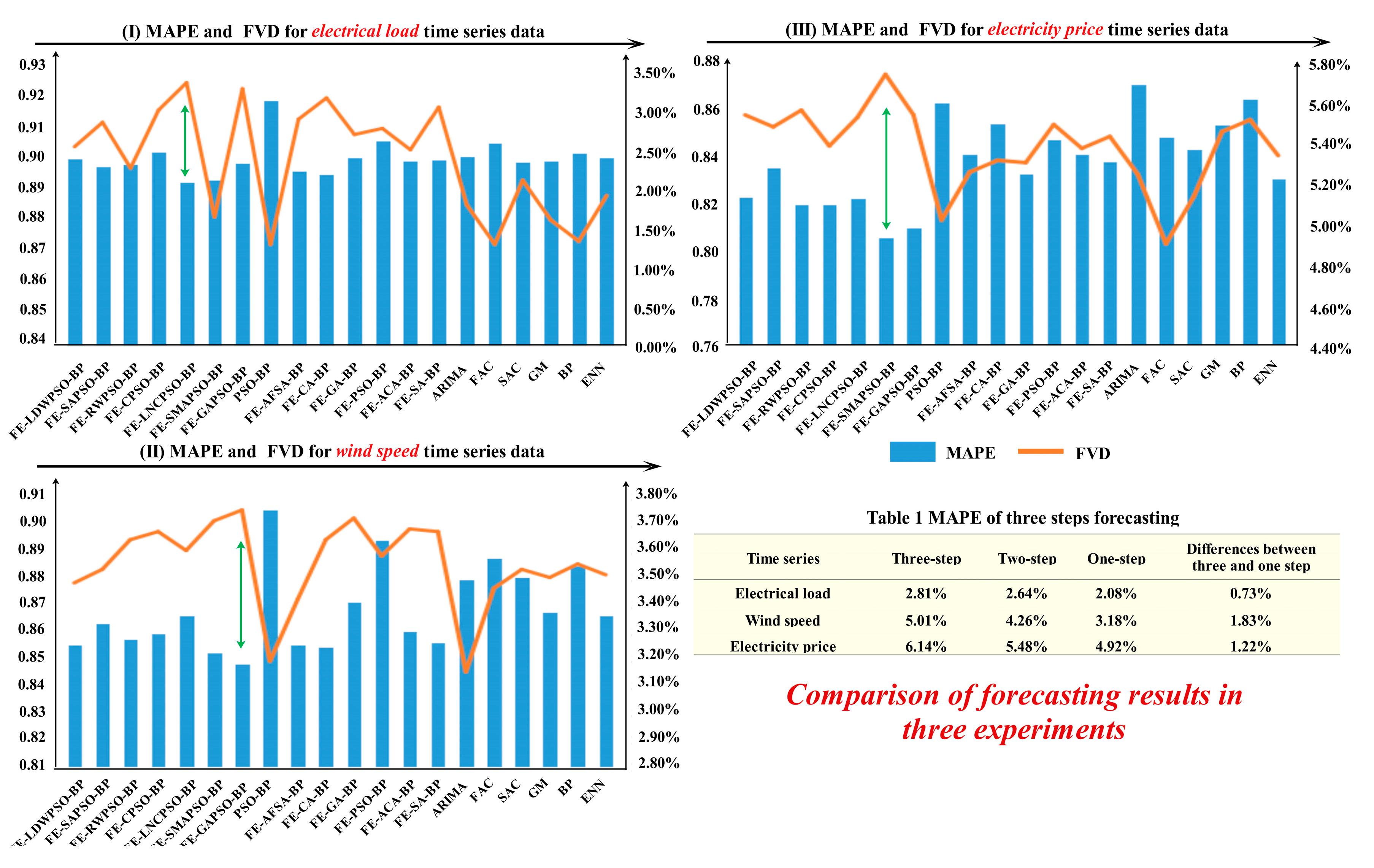
First of all, for the comparison of FE-NPSO-BP, in one-step forecasting, LNCPSO has the best MAPE, MAE and FVD at 2.08%, 85.468 and 0.926, respectively. GAPSO achieves better MSE in one-step forecasting. For three-step forecasting, RWPSO has the lowest MAPE, at 2.72%. The forecasting error between the combined PSO and modified PSO is small. Therefore, in summary, the forecasting result is similar for modified PSO and combined PSO when forecasting electoral load time series.

(b)

For BP optimized by different algorithms, in one-step forecasting, FE-CA-BP has the lowest MAPE, which is 2.18%. FE-PSO-BP and FE-ACA-BP have the best MAPE with 2.69% and 2.90%. For the other indexes, different models achieve different values. Therefore, it can be summarized that BP optimized by other single optimization algorithms is less stable, and it is difficult to find a suitable method to forecast the electrical load time series accurately.

(c)

Finally, compared to conventional models, GM has the best forecasting performance, and the MAPE is 2.96% and 2.25% in three-step and one-step forecasting, respectively. The MAPE of ARIMA in two-step forecasting is 2.77%. In general, the performance of machine-learning-based methods is better than for traditional statistical models.

Remark 11. 

In one-step forecasting, the forecasting accuracy of the electrical load time series is approximately 2% because the time series is more regular. The results show that the effects of the modified and combined particle swarm optimization are similar. FE-NPSO-BP outperforms both conventional models and BP optimized by other algorithms.

4.5. Experiment II

Table 4. Comparison of hybrid models with different optimization algorithms and conventional models for wind speed time series.

Different Improved PSO	FE-LDWPSO-BP			FE-SAPSO-BP			FE-RWPSO-BP			FE-CPSO-BP
	Three-step	Two-step	One-step	Three-step	Two-step	One-step	Three-step	Two-step	One-step	Three-step	Two-step	One-step
MAPE	5.38%	4.38%	3.25%	5.35%	4.52%	3.33%	5.44%	4.49%	3.27%	5.28%	4.71%	3.29%
MAE (m/s)	1.354	0.899	0.528	1.469	0.904	0.621	1.183	0.945	0.613	1.448	1.106	0.753
MSE (104 m/s2)	0.624	0.531	0.456	0.608	0.497	0.386	0.594	0.493	0.374	0.618	0.523	0.406
FVD	0.813	0.854	0.878	0.826	0.846	0.883	0.834	0.862	0.894	0.855	0.880	0.897
Index	FE-LNCPSO-BP			FE-SMAPSO-BP			FE-GAPSO-BP			PSO-BP
	Three-step	Two-step	One-step	Three-step	Two-step	One-step	Three-step	Two-step	One-step	Three-step	Two-step	One-step
MAPE	5.21%	4.67%	3.36%	4.99%	4.52%	3.22%	5.01%	4.26%	3.18%	5.96%	4.93%	3.75%
MAE (m/s)	1.443	0.824	0.529	0.912	0.614	0.505	1.154	0.718	0.417	1.689	1.441	0.820
MSE (104 m/s2)	0.593	0.478	0.396	0.608	0.453	0.325	0.578	0.429	0.331	0.662	0.593	0.512
FVD	0.842	0.866	0.890	0.861	0.882	0.901	0.852	0.873	0.905	0.808	0.823	0.849
Optimization algorithms	FE-AFSA-BP			FE-CA-BP			FE-GA-BP			FE-PSO-BP
	Three-step	Two-step	One-step	Three-step	Two-step	One-step	Three-step	Two-step	One-step	Three-step	Two-step	One-step
MAPE	5.18%	4.89%	3.25%	5.63%	4.44%	3.24%	5.37%	4.76%	3.41%	5.22%	4.65%	3.64%
MAE (m/s)	1.226	0.941	0.651	1.287	0.809	0.543	1.449	0.978	0.503	1.287	0.835	0.498
MSE (104 m/s2)	0.612	0.513	0.376	0.582	0.453	0.374	0.605	0.583	0.426	0.557	0.429	0.351
FVD	0.841	0.866	0.872	0.837	0.859	0.894	0.826	0.861	0.902	0.837	0.865	0.888
Index	FE-ACA-BP			FE-SA-BP
	Three-step	Two-step	One-step	Three-step	Two-step	One-step
MAPE	5.48%	4.71%	3.30%	5.35%	4.73%	3.26%
MAE (m/s)	1.183	0.844	0.527	1.319	1.003	0.628
MSE (104 m/s2)	0.623	0.476	0.395	0.606	0.504	0.359
FVD	0.831	0.863	0.898	0.822	0.854	0.897
Conventional algorithms	ARIMA			FAC			SAC			GM
	Three-step	Two-step	One-step	Three-step	Two-step	One-step	Three-step	Two-step	One-step	Three-step	Two-step	One-step
MAPE	5.66%	4.59%	3.49%	5.59%	4.72%	3.57%	5.48%	4.63%	3.50%	5.31%	4.70%	3.37%
MAE (m/s)	1.738	0.696	0.421	1.824	1.548	1.039	1.626	1.117	0.945	1.593	1.215	0.786
MSE (104 m/s2)	0.683	0.626	0.519	0.662	0.594	0.417	0.602	0.517	0.385	0.599	0.452	0.378
FVD	0.802	0.812	0.845	0.826	0.844	0.876	0.845	0.855	0.883	0.826	0.858	0.880
Index	BP			ENN
	Three-step	Two-step	One-step	Three-step	Two-step	One-step
MAPE	5.62%	4.71%	3.54%	5.49%	4.55%	3.36%
MAE (m/s)	1.446	1.217	0.863	1.349	0.827	0.663
MSE (104 m/s2)	0.617	0.489	0.367	0.588	0.429	0.377
FVD	0.841	0.868	0.885	0.829	0.847	0.881

shows the forecasting results of the wind speed time series, which is less regular than the electrical load time series. The forecasting of wind speed is a challenging task. This section demonstrates the forecasting results using the hybrid models put forward in this paper. The findings are listed below:

(a)

For the short-term wind speed time series and all forecasting steps, the combined PSO algorithms achieve better forecasting accuracy. GAPSO has the best forecasting results, with a MAPE of 3.18% and an FVD of 0.905 in one-step forecasting. In comparison, PSO-BP has the worst performance, and the MAPE increases by 0.57% compared with GAPSO because FEEMD denoises the original time series and makes the processed data smoother. It can be concluded that the combined algorithms are more effective in forecasting the short-term wind speed, which is because GA has a stronger ability to search for the global optimum and achieve a faster rate of convergence.

(b)

Among the separate types of optimization algorithms, FE-CA-BP and FE-AFSA-BP have the best forecasting performance. In comparison, the proposed hybrid model, FE-GAPSO-BP, increases the forecasting accuracy by 0.06%, 0.18% and 0.17%. The forecasting differences among different types of optimization algorithms are not significant.

(c)

When comparing the proposed hybrid models with traditional forecasting methods, BP, ENN and GM achieve the best MAPE, with 3.31%, 4.55% and 5.31%. Although ARIMA has better MAEs in one- and two-step forecasting, the other indexes such as MSE and FVD are worse. BP has a better FVD, but its forecasting performance is worse than that of GAPSO because the output of the single BP is not stable and has a relatively low capability for fault tolerance.

Remark 12. 

The proposed FE-NPSO-BP outperforms the other traditional forecasting models, and the artificial intelligence neural network has better forecasting performance than traditional statistical models. The forecasting accuracy for short-term wind speed is approximately 3.2%.

4.6. Experiment III

Experiment III was designed to verify the effectiveness of the proposed hybrid models using the electricity price time series. If the hybrid models are applicable and suitable, it can be concluded that the proposed hybrid models are effective in forecasting the electric power system, which is because the electricity price is the most irregular one compared to the above two time series.

Table 5. Comparison of hybrid models with different optimization algorithms and conventional models for electricity price time series.

Different Improved PSO	FE-LDWPSO-BP			FE-SAPSO-BP			FE-RWPSO-BP			FE-CPSO-BP
	Three-step	Two-step	One-step	Three-step	Two-step	One-step	Three-step	Two-step	One-step	Three-step	Two-step	One-step
MAPE	6.26%	5.75%	5.12%	6.33%	5.79%	5.26%	6.27%	5.66%	5.08%	6.21%	5.77%	5.08%
MAE (m/s)	4.217	3.624	2.995	4.033	3.719	2.464	3.965	3.421	2.467	3.421	3.056	2.429
MSE (104 m/s2)	47.628	39.175	20.006	25.498	23.127	16.514	39.672	24.194	19.554	32.177	22.316	20.007
FVD	0.794	0.829	0.856	0.787	0.825	0.851	0.786	0.833	0.858	0.762	0.815	0.843
Index	FE-LNCPSO-BP			FE-SMAPSO-BP			FE-GAPSO-BP			PSO-BP
	Three-step	Two-step	One-step	Three-step	Two-step	One-step	Three-step	Two-step	One-step	Three-step	Two-step	One-step
MAPE	6.39%	5.50%	5.11%	6.14%	5.48%	4.92%	6.23%	5.50%	4.97%	7.18%	6.14%	5.58%
MAE (m/s)	4.116	3.547	2.469	3.858	3.129	2.318	3.964	3.252	2.179	4.665	4.193	3.217
MSE (104 m/s2)	41.759	30.625	22.479	35.175	21.428	18.176	30.987	23.165	18.550	56.423	44.229	30.706
FVD	0.782	0.831	0.855	0.801	0.845	0.873	0.775	0.824	0.856	0.742	0.808	0.812
Optimization algorithms	FE-AFSA-BP			FE-CA-BP			FE-GA-BP			FE-PSO-BP
	Three-step	Two-step	One-step	Three-step	Two-step	One-step	Three-step	Two-step	One-step	Three-step	Two-step	One-step
MAPE	6.31%	5.68%	5.33%	6.46%	5.92%	5.48%	6.44%	5.71%	5.23%	6.17%	5.81%	5.40%
MAE (m/s)	4.331	3.902	2.886	4.174	3.628	2.596	4.333	3.714	2.467	4.195	3.812	2.759
MSE (104 m/s2)	44.138	33.965	23.004	44.239	33.547	22.695	43.996	35.368	22.510	37.474	26.615	18.691
FVD	0.774	0.815	0.832	0.789	0.830	0.837	0.762	0.829	0.836	0.760	0.824	0.852
Index	FE-ACA-BP			FE-SA-BP
	Three-step	Two-step	One-step	Three-step	Two-step	One-step
MAPE	6.25%	5.94%	5.33%	6.45%	5.70%	5.29%
MAE (m/s)	4.118	3.956	2.741	4.208	3.595	2.617
MSE (104 m/s2)	31.098	28.667	21.094	42.065	36.172	23.108
FVD	0.790	0.816	0.842	0.741	0.825	0.847
Conventional algorithms	ARIMA			FAC			SAC			GM
	Three-step	Two-step	One-step	Three-step	Two-step	One-step	Three-step	Two-step	One-step	Three-step	Two-step	One-step
MAPE	6.57%	5.92%	5.67%	6.62%	6.08%	5.41%	6.31%	5.94%	5.35%	6.41%	5.68%	5.47%
MAE (m/s)	4.083	3.172	2.338	4.125	3.519	2.443	4.098	3.252	2.419	4.396	3.772	2.983
MSE (104 m/s2)	49.176	44.155	36.128	46.008	24.019	18.662	49.216	39.205	23.178	42.074	35.102	20.316
FVD	0.753	0.792	0.831	0.730	0.768	0.802	0.765	0.815	0.822	0.783	0.824	0.849
Index	BP			ENN
	Three-step	Two-step	One-step	Three-step	Two-step	One-step
MAPE	6.33%	5.96%	5.60%	6.25%	5.84%	5.21%
MAE (m/s)	4.275	3.628	2.416	4.226	3.823	2.796
MSE (104 m/s2)	38.429	24.108	19.337	39.219	25.441	23.053
FVD	0.761	0.829	0.854	0.786	0.825	0.839

shows the comparison results.

(a)

For the electricity price time series, SMAPSO has the lowest MAPE and the highest FVD. The MAPE values for GAPSO are similar to the values for SMAPSO, which means that the combined PSO algorithm is more effective in forecasting the electricity price. In one-step forecasting, SMAPSO increases the forecasting accuracy by 0.66%.

(b)

When comparing different types of algorithms, the MAPE value of FE-SA-BP is the best, with 5.29% for one-step forecasting, the MAPE of FE-AFSA-BP achieves the best value of 5.68% for two-step forecasting, and FE-PSO-BP has the best MAPE at 6.17%. BP optimized by NPSOs outperforms the other algorithms, including AFSA, CA, GA, PSO, ACA and SA. Therefore, the combination of algorithms can adopt the advantages of the single ones. Both the ability to search for the global optimum and the convergence rate are enhanced.

(c)

Finally, consistent with the results of the electrical load and wind speed time series data, the machine-learning-based algorithms have better forecasting performance than the conventional algorithms, such as ARIMA, FAC and SAC, because the indexes of MAE, MSE and FVD are all better as well.

Remark 13. 

Based on this comparison, it could be summarized that the hybrid models optimized by the improved particle swarm optimization algorithms perform better than the other types of optimization algorithms, further proving the effectiveness of the model. Moreover, the difference between one-step and three-step forecasting is small and is on an acceptable scale. Therefore, the proposed hybrid models are concluded to be suitable for multi-step forecasting. The forecasting accuracy for the electricity price is approximately 5%.

Figure 5 compares the results of the hybrid models. The bar chart represents the MAPE, and the line chart represents the FVD. The figure shows that for the electrical load time series, FE-LNCPSO-BP has the lowest MAPE and highest FVD. For the wind speed time series, FE-GAPSO-BP achieves the best MAPE and FVD. For the electricity price time series, FE-SMAPSO-BP has the lowest MAPE and the best FVD. The figure clearly shows the performance of each forecasting model. Furthermore, the table presents the forecasting MAPE for the three steps. We find that the MAPE differences between one-step and three-step forecasting for the three time series data are 0.73%, 1.83% and 1.22%, respectively, which is acceptable.

5. Discussion

This section aims to present a deeper discussion of the experimental results, including statistical models, artificial intelligence neural networks, each part in the hybrid model, forecasting steps and running time.

5.1. Statistical Model

As is well known, traditional statistical models include AR, ARMA, ARIMA, FAC and SAC. ARIMA is the next-generation form of ARMA and has a higher forecasting accuracy. In this paper, we only apply ARIMA to conduct the forecasting. For the short-term wind speed time series and the electrical load time series, it has higher forecasting accuracy than BP. For the electricity price time series, its forecasting performance is worse. The basic form of ARIMA is ARIMA (p, q, d). The models could be fitted by least squares regressions to find the values of the parameters, which could minimize the error term after p and q are set. Akaike information criterion (AICs) are applied to judge whether p and q are the best [55]. In our experiments, the form of ARIMA for both short-term wind speed and electricity price is ARIMA (3,2,1). For the electrical load time series, the form of ARIMA is ARIMA (3,3,1). The other two models are FAC and SAC. The aim of FAC is to correct the coefficient values constantly based on changes in data for the best forecasting results. SAC is an improvement based on FAC. The experiments above reveal that their forecasting accuracy is worse than that of ARIMA. Although traditional statistical models are used widely in electrical system forecasting, they are more applicable in forecasting linear trends: in other words, it is required that the original data should be smooth without high fluctuation.

5.2. Artificial Intelligence Neural Network

As a comparison, the artificial intelligence neural networks are suitable for forecasting non-linear data trends, and this paper contrasts the hybrid models with GM, ENN and BPNN. In the three experiments, the hybrid models proposed all achieve the best forecasting accuracy. The forecasting performance of GM for the electrical load time series is better than the other models, with MAPE values of 2.34%, 2.79% and 2.96%, respectively. However, the forecasting results of BPNN are worse than for the traditional statistical models, such as ARIMA, FAC and SAC, because the network of BPNN is not stable. Therefore, to improve the stability of the network of BPNN and thus the forecasting accuracy, this paper introduces improved PSO to optimize the weight and threshold of BPNN. The experiments above show that the optimized BPNN combines the advantages of each single model, and the forecasting accuracy is improved. As is well known, the three data sequences in the electrical system all have irregular distributions with high fluctuation and substantial noise. Thus, NNs are more applicable when forecasting the indicators in the electrical system due to the training and testing mechanism and the high error tolerance. We also explore the influence of the training and verification ratio on the forecasting results. In addition to 15:1 and 5:1 ratios of training and verification, we also set the value to 3:1, 6:1 10:1 and 12:1. The final results demonstrate that there is no close relationship between the training and verification ratio and the forecasting accuracy. To summarize, although NNs still have some limitations, they are the fittest models for forecasting the indicators in the electrical system after the parameters in the network are optimized and the original data are preprocessed.

5.3. Significance of Forecasting Results

In this part, the significance of the forecasting performance of the proposed models is tested by using the DM test. The pairwise comparisons of the forecasting models are summarized in

Table 6. Summary of DM test (values of DM are absolute values).

Model	Electrical Load		Wind Speed		Electricity Price
	DM	p-Value	DM	p-Value	DM	p-Value
FE-LDWPSO-BP	3.657	0.0134	0.8984	0.8661	2.146	0.0142
FE-SAPSO-BP	0.264	0.7581	2.154	0.0000	2.135	0.0112
FE-RWPSO-BP	3.448	0.0065	1.356	0.6849	2.031	0.0234
FE-CPSO-BP	3.998	0.0000	1.559	0.6594	1.983	0.0252
FE-SMAPSO-BP	0.0842	0.9283	2.185	0.0000	2.066	0.0168
FE-GAPSO-BP	3.469	0.0082	0.128	0.9164	1.359	0.7426
PSO-BP	4.375	0.0000	2.965	0.0000	2.836	0.0000
FE-AFSA-BP	0.255	0.7076	0.731	0.8642	2.328	0.0000
FE-CA-BP	0.237	0.6438	0.545	0.8776	2.736	0.0000
FE-GA-BP	3.718	0.0000	2.139	0.0000	2.174	0.0155
FE-PSO-BP	4.092	0.0000	2.772	0.0000	2.669	0.0000
FE-ACA-BP	3.613	0.0000	2.063	0.0000	2.396	0.0000
FE-SA-BP	3.658	0.0000	1.242	0.7015	2.223	0.0000
ARIMA	3.826	0.0000	2.356	0.0000	2.979	0.0000
FAC	3.987	0.0000	2.246	0.0000	2.647	0.0000
SAC	3.472	0.0000	2.385	0.0000	2.528	0.0000
GM	3.566	0.0000	2.246	0.0000	2.699	0.0000
BP	3.885	0.0000	2.417	0.0000	2.874	0.0000
ENN	3.779	0.0000	2.209	0.0000	2.008	0.0197

. The null hypothesis is that there are no observed differences between the performances of two forecasting models, while the alternative hypothesis is that the observed differences between the performances of two forecasting models are significant. For the electrical load time series data, the most suitable model is FE-LNCPSO-BP, so it is compared with the other models. The results show that the differences between FE-LNCPSO-BP and FE-SAPSO-BP, FE-SMAPSO-BP, FE-AFSA-BP, and FE-CA-BP are not significant, which indicates that both combined and modified PSO can forecast the electrical load time series accurately. There is a significant difference between FE-LNCPSO-BP and the other compared models. For the wind speed time series data, FE-GAPSO-BP is the most suitable model, and the results of the DM test show that the differences between FE-GAPSO-BP and FE-LDWPSO-BP, FE-RWPSO-BP, FE-CPSO-BP, FE-SMAPSO-BP, FE-AFSA-BP, and FE-SA-BP are not significant. Therefore, the proposed hybrid models are more effective than the other models. Finally, for electricity price forecasting, FE-GAPSO-BP is the only model with no significant difference from FE-SMAPSO-BP. The other models all exhibit significant differences from FE-SMAPSO-BP. Thus, based on these results, we know that the combined models are more suitable for less regular time series data than the modified models.

5.4. Discussion of the Effectiveness of Fast Ensemble Empirical Mode Decomposition

The data in the electrical system are irregular and include high fluctuation with noise, so it is very important to denoise the original data sequences before conducting the forecasting. In this paper, FEEMD is applied to denoise the original time series data. By comparing the forecasting results of PSO-BP with the results of FE-PSO-BP, we can testify to the effectiveness of FEEMD, which was found to increase the forecasting accuracy greatly: FEEMD increases the MAPE by 0.96%, 0.11% and 0.18% for the electrical load time series, short-term wind speed time series, and electricity price time series, respectively. In addition to the improvement of the MAPE, the FVD also increases substantially, to 0.038, 0.039 and 0.040, respectively. Therefore, FEEMD not only contributes to the forecasting accuracy but also can help increase the FVD. Furthermore, this paper removes the first two IMFs, and the rest are utilized in the forecasting. To deeply explore the effectiveness of FEEMD, we also implement experiments that remove the first three, four and five IMFs and judge whether the forecasting results are affected. The results demonstrate that when the first two columns are removed, the forecasting accuracy is the best, as in our experiment.

5.5. Comparison of Different Types of Particle Swarm Optimization Algorithms

The improved particle swarm optimization algorithm could be divided into two parts. One part is to introduce the advanced theory into the particle swarm optimization algorithm, and the other is to combine the particle swarm optimization algorithm with other intelligent optimization algorithms. First, in the discussion above, the initial method of modifying the particle swarm optimization algorithm is to adjust its inertia weight. The linearly decreasing inertia weight particle swarm optimization algorithm contributes to obtaining the best solution; however, it still has three drawbacks. The first drawback is that the linearly decreasing inertia weight reduces the convergence rate of the algorithm. The second drawback is that the algorithm is prone to falling into a local optimum because the local search ability of the algorithm is weak at the beginning, and the global search capacity is weak at the end. The final drawback is that it is difficult to forecast the maximum number of iterations, which affects the regulatory function of the algorithm.

Thus, to balance the searching ability of the local and global optimums, the adjustment of non-linear inertia weights is incorporated, including the self-adaptive inertia weight particle swarm optimization and random weight particle swarm optimization. In the former technique, the inertia weight changes along with the value of the fitness. For the latter technique, choosing the inertia weight randomly could overcome the disadvantages of the linearly decreasing method mentioned above. In addition to the inertia weight, the learning factor also plays a significant role in improving the efficiency of the particle swarm optimization algorithm. The learning factor would affect the flying velocity of each particle, and, thus, the introduction of the constriction factor is beneficial for controlling the flying velocity and enhancing the local searching ability of the particles compared to the adjustment of the inertia weight.

The second method is to combine other algorithms with the particle swarm optimization algorithm to overcome the disadvantages of a single algorithm. The combination with simulated annealing is simple to conduct and improves the ability to seek the global optimum, simultaneously enhancing the rate of convergence and the accuracy of the algorithm. The combination of GA and particle swarm optimization also strengthens the convergence rate and improves the convergence accuracy.

The experimental results demonstrate that the combination of particle swarm optimization with other algorithms is more effective when the forecasting accuracy is approximately 4%. However, for high forecasting accuracy, such as for the electrical load time series, there is no great difference between the different types of algorithms.

5.6. Selection of the Hidden and Input Layers for Back Propagation

This paper applies BPNN, the most common and effective artificial intelligence neural network in practical application, for forecasting in the electrical system. However, BPNN possesses some drawbacks: for example, its output results are unstable due to the instability of learning and memory, and its convergence rate is slow. Therefore, two key parameters, the weight and threshold values, are optimized by the optimization algorithms in this paper to obtain a more valid hybrid model. Moreover, the selection of hidden layers is a highly complicated problem that requires more experience and several experiments, as there is no ideal analysis formula to calculate the hidden layers. The number of input layers and hidden layers of the BP neural network has a direct relationship with the forecasting accuracy. When the number is too small, there is not enough information for the network to learn; similarly, when the number is too large, it not only increases the training time but also leads to too much time for learning. Under that condition, the error may not be optimal. Furthermore, the large number of input layers and hidden layers would also lead to low fault tolerance, making it difficult for the neural network to identify the samples that are not trained. Furthermore, the overfitting problem cannot be ignored: the increasing error results in the decreasing generalization ability. Therefore, it is crucial to select an appropriate number of hidden layers. In our experiments, the listing technique is applied to choose the input layers and hidden layers.

Table 7. Selection of input layers and hidden layers of BP neural network (MAPE).

Hidden Layer	Input Layer
	3	4	5	6		3	4	5	6
Electrical load time series
5	2.95%	2.86%	2.72%	2.88%	11	2.98%	2.82%	3.07%	2.94%
6	2.88%	2.83%	2.75%	2.71%	12	2.76%	2.75%	3.11%	2.93%
7	2.76%	2.68%	2.79%	2.88%	13	2.69%	2.81%	3.15%	3.01%
8	2.82%	2.71%	2.84%	2.92%	14	2.74%	2.92%	2.94%	2.85%
9	2.67%	2.81%	2.72%	3.06%	15	2.88%	2.95%	2.83%	2.89%
10	2.92%	2.90%	2.89%	3.09%	16	2.92%	2.74%	2.70%	2.94%
Short-term wind speed time series
5	5.10%	4.99%	4.98%	5.08%	11	5.12%	5.14%	5.21%	5.24%
6	5.12%	4.93%	5.35%	5.00%	12	4.99%	5.24%	5.31%	5.11%
7	5.04%	5.00%	5.42%	5.09%	13	5.05%	5.19%	5.16%	4.99%
8	5.22%	5.21%	5.17%	5.15%	14	5.17%	5.03%	5.08%	5.32%
9	4.98%	5.15%	5.03%	5.23%	15	5.21%	5.06%	4.99%	5.20%
10	5.17%	5.14%	5.16%	5.14%	16	5.05%	5.18%	5.31%	5.39%
Electricity price time series
5	5.92%	5.91%	5.90%	5.77%	11	5.79%	5.81%	6.11%	5.85%
6	5.71%	5.84%	5.87%	5.88%	12	5.84%	5.94%	6.03%	5.80%
7	6.11%	6.06%	5.89%	6.09%	13	5.84%	5.96%	5.92%	5.81%
8	6.02%	6.18%	5.91%	5.99%	14	5.86%	5.85%	5.84%	5.96%
9	5.85%	5.84%	5.92%	5.90%	15	6.07%	6.08%	6.18%	5.97%
10	5.78%	5.81%	6.12%	5.83%	16	5.99%	6.14%	6.23%	5.91%

shows that when the number of input layers is four and the number of hidden layers is six, BPNN has the best forecasting accuracy for the short-term wind speed time series. When the number of input layers is three and the number of hidden layers is nine, BPNN achieves higher forecasting accuracy for the electrical load time series. When the numbers of input layers and hidden layers are three and six, respectively, the forecasting error of BPNN for electricity price is the smallest.

5.7. Steps of Forecasting

To verify the effectiveness of the proposed hybrid model, this paper conducts multi-step forecasting, including one-step, two-step and three-step forecasting, for the three indicators in the electrical system.

Table 8. Comparison of multi-step forecasting accuracy.

	One-Step	Two-Step	Improvement	Three-Step	Improvement
Electrical load time series
MAPE	2.08%	2.64%	0.56%	2.81%	0.73%
MAE (m/s)	85.468	92.473	7.005	96.698	11.230
MSE (104 m/s2)	1.338	1.583	0.245	2.176	0.838
FVD	0.926	0.915	0.011	0.896	0.03
Short-term wind speed time series
MAPE	3.18%	4.26%	1.08%	5.01%	1.83%
MAE (m/s)	0.417	0.718	0.301	1.154	0.737
MSE (m/s2)	0.331	0.429	0.098	0.578	0.247
FVD	0.905	0.873	0.032	0.852	0.053
Electricity price time series
MAPE	4.92%	5.48%	0.56%	6.14%	1.22%
MAE (m/s)	2.318	3.129	0.811	3.858	1.540
MSE (m/s2)	18.176	21.428	3.252	35.175	16.999
FVD	0.873	0.845	0.028	0.801	0.072

compares the multi-step forecasting accuracy. For the electrical load time series, the forecasting accuracy of one-step forecasting increases by 0.56% and 0.73% compared with three-step forecasting and two-step forecasting. For the wind speed time series, the difference between one-step forecasting and two-step and three-step forecasting is 1.08% and 1.83%, respectively. For the electricity price time series, the forecasting accuracy improves by 0.56% and 1.22%, respectively. In other words, the difference between one-step and three-step forecasting is within 2%, which is on an acceptable scale. Furthermore, it is proven that the hybrid model proposed is suitable for multi-step forecasting. The optimization of the parameters in BPNN allows the forecasting model to obtain more accurate results, using its advantages to compensate for the shortcomings of the other component models, which demonstrates the superiority of the proposed hybrid models [61].

5.8. Running Time

Table 9. Comparison of performance times for hybrid models.

Model	Time (s)	Model	Time (s)
FE-LDWPSO-BP	84.28	FE-SMAPSO-BP	118.73
FE-SAPSO-BP	114.52	FE-AFSA-BP	138.74
FE-RWPSO-BP	71.33	FE-CA-BP	161.49
FE-CPSO-BP	93.10	FE-GA-BP	92.18
FE-LNCPSO-BP	85.21	FE-ACA-BP	107.22
FE-SA-BP	112.55

compares the results of the performance time for the experiments using different algorithms on all of the data sets, implemented on Windows 8.1 with a 2.5 GHz Intel Core i5-4200U, 64 bit with 4GB RAM. FE-RWPSO-BP has the shortest running time, at 71.33 s. FE-CA-BP has the longest running time, at 161.49 s. In comparison, the running time of the FE-NPSO-BP models is within two minutes, which also testifies to the good forecasting performance of the hybrid models. They are applicable for forecasting short-term wind speed with a 10 min interval and electrical load and electricity price with a 30 min interval.

6. Conclusions

Electrical power systems always play an important part in the planning of national and regional economic development. The following three key indicators in the electrical power system are forecasted here: the short-term wind speed, electrical load and electricity price. All of these indicators contain a large amount of information related to the generation, distribution and trade of electricity. However, it is difficult to implement accurate forecasting due to the high fluctuation and noise in the original data sequences. This paper proposes a series of hybrid models called FE-NPSO-BP to explore how to attain better forecasting performance. The electrical load time series is the most regular; therefore, it is easier to achieve a higher forecasting accuracy of approximately 2%. In comparison, the electricity price is the most irregular; thus, its forecasting accuracy is lower, with an approximate value over 4%. The wind speed time series data are intermediate compared to the other two. In our experiments, we found that combined PSO algorithms are more effective for irregular time series data than modified PSO algorithms. However, when the time series data tend to be regular, both combined and modified PSO algorithms are suitable for forecasting. In one-step forecasting, GAPSO, LNCPSO and SMAPSO are the most suitable models for the short-term wind speed, electrical load and electricity price time series. Moreover, the presented models are designed to be easily parallelizable, and, thus, they can perform the learning process over a large data set in a limited amount of time. Both the forecasting accuracy and running time of the hybrid models demonstrate their effectiveness in time series forecasting for electrical power systems.

References

1. Wang, J.Z.; Hu, J.M.; Ma, K.L.; Zhang, Y.X. A self-adaptive hybrid approach for wind speed forecasting. Renew. Energy 2015, 78, 374–385. [Google Scholar] [CrossRef]
2. Ladislav, Z. Wind speed forecast correction models using polynomial neural networks. Renew. Energy 2015, 83, 998–1006. [Google Scholar]
3. Lu, X.; Wang, J.Z.; Cai, Y.; Zhao, J. Distributed HS-ARTMAP and its forecasting model for electricity load. Appl. Soft Comput. 2015, 32, 13–22. [Google Scholar] [CrossRef]
4. Koprinska, I.; Rana, M.; Agelidis, V.G. Correlation and instance based feature selection for electricity load forecasting. Knowl.-Based Syst. 2015, 82, 29–40. [Google Scholar] [CrossRef]
5. Kaytez, F.; Taplamacioglu, M.C.; Cam, E.; Hardalac, F. Forecasting electricity consumption: A comparison of regression analysis, neural networks and least squares support vector machines. Int. J. Electr. Power 2015, 67, 431–438. [Google Scholar] [CrossRef]
6. Raviv, E.; Bouwman, K.E.; Dijk, D.V. Forecasting day-ahead electricity prices: Utilizing hourly prices. Energy Econ. 2015, 50, 227–239. [Google Scholar] [CrossRef]
7. Liu, H.; Tian, H.Q.; Liang, X.F.; Li, Y.F. Wind speed forecasting approach using secondary decomposition algorithm and Elman neural networks. Appl. Energy 2015, 157, 183–194. [Google Scholar] [CrossRef]
8. Raza, M.Q.; Khosravi, A. A review on artificial intelligence based load demand forecasting techniques for smart grid and buildings. Renew. Sust. Energy Rev. 2015, 50, 1352–1372. [Google Scholar] [CrossRef]
9. Kavasseri, R.G.; Seetharaman, K. Day-ahead wind speed forecasting using f-ARIMA models. Renew. Energy 2009, 34, 1388–1393. [Google Scholar] [CrossRef]
10. Wang, Y.Y.; Wang, J.Z.; Zhao, G.; Dong, Y. Application of residual modification approach in seasonal ARIMA for electricity demand forecasting: A case study of China. Energy Policy 2012, 48, 284–294. [Google Scholar] [CrossRef]
11. Shukur, O.B.; Lee, M.H. Daily wind speed forecasting through hybrid KF-ANN model based on ARIMA. Renew. Energy 2015, 76, 637–647. [Google Scholar] [CrossRef]
12. Babu, C.N.; Reddy, B.E. A moving-average filter based hybrid ARIMA-ANN model for forecasting time series data. Appl. Soft Comput. 2014, 23, 27–38. [Google Scholar] [CrossRef]
13. Cadenas, E.; Rivera, W. Wind speed forecasting in three different regions of Mexico, using a hybrid ARIMA-ANN model. Renew. Energy 2010, 35, 2732–2738. [Google Scholar] [CrossRef]
14. Yahyai, S.A.; Charabi, Y.; Gastli, A. Review of the use of numerical weather prediction (NWP) models for wind energy assessment. Renew. Sust. Energy Rev. 2010, 14, 3192–3198. [Google Scholar] [CrossRef]
15. Zhang, J.; Draxl, C.; Hopson, T.; Monache, L.D.; Vanvyve, E.; Hodge, B.M. Comparison of numerical weather prediction based deterministic and probabilistic wind resource assessment methods. Appl. Energy 2015, 156, 528–541. [Google Scholar] [CrossRef]
16. Giorgi, M.G.; Ficarella, A.; Tarantino, M. Assessment of the benefits of numerical weather predictions in wind power forecasting based on statistical methods. Energy 2011, 36, 3968–3978. [Google Scholar] [CrossRef]
17. Felice, M.D.; Alessandri, A.; Ruti, P.M. Electricity demand forecasting over Italy: Potential benefits using numerical weather prediction models. Electr. Power Syst. Res. 2013, 104, 71–79. [Google Scholar] [CrossRef]
18. Sile, T.; Bekere, L.; Frisfelde, D.C.; Sennikovs, J.; Bethers, U. Verification of numerical weather prediction model results for energy applications in Latvia. Energy Procedia 2014, 59, 213–220. [Google Scholar] [CrossRef]
19. Patterson, D.W. Artificial Neural Networks: Theory and Applications; Prentice Hall PTR: Upper Saddle River, NJ, USA, 1998. [Google Scholar]
20. Liu, H.; Tian, H.Q.; Liang, X.F.; Li, Y.F. New wind speed forecasting approaches using fast ensemble empirical model decomposition, genetic algorithm, mind evolutionary algorithm and artificial neural networks. Renew. Energy 2015, 83, 1066–1075. [Google Scholar] [CrossRef]
21. Lou, C.W.; Dong, M.C. A novel random fuzzy neural networks for tackling uncertainties of electric load forecasting. Int. J. Electr. Power 2015, 73, 34–44. [Google Scholar] [CrossRef]
22. Coelho, L.; Santos, A. A RBF neural network model with GARCH errors: Application to electricity price forecasting. Electr. Power Syst. Res. 2011, 81, 74–83. [Google Scholar] [CrossRef]
23. Keles, D.; Scelle, J.; Paraschiv, F.; Fichtner, W. Extended forecast methods for day-ahead electricity spot prices applying artificial neural networks. Appl. Energy 2016, 162, 218–230. [Google Scholar] [CrossRef]
24. Anbazhagan, S.; Kumarappan, N. A neural network approach to day-ahead deregulated electricity market prices classification. Electr. Power Syst. Res. 2012, 86, 140–150. [Google Scholar] [CrossRef]
25. Wang, W.N.; Liu, X.D. Fuzzy forecasting based on automatic clustering and axiomatic fuzzy set classification. Inform. Sci. 2015, 294, 78–94. [Google Scholar] [CrossRef]
26. Zhao, F.Q.; Liu, Y.; Zhang, C.; Wang, J.B. A self-adaptive harmony PSO search algorithm and its performance analysis. Expert Syst. Appl. 2015, 42, 7436–7455. [Google Scholar] [CrossRef]
27. Chung, S.H.; Chan, H.K.; Chan, F.T.S. A modified genetic algorithm for maximizing handling reliability and recyclability of distribution centers. Expert Syst. Appl. 2013, 40, 7588–7595. [Google Scholar] [CrossRef]
28. Arce, T.; Román, P.E.; Velásquez, J.; Parada, V. Identifying web sessions with simulated annealing. Expert Syst. Appl. 2014, 41, 1593–1600. [Google Scholar] [CrossRef]
29. Leung, S.Y.S.; Tang, Y.; Wong, W.K. A hybrid particle swarm optimization and its application in neural networks. Expert Syst. Appl. 2012, 39, 395–405. [Google Scholar] [CrossRef]
30. Xiao, J.; Ao, X.T.; Tang, Y. Solving software project scheduling problems with ant colony optimization. Comput. Oper. Res. 2013, 40, 33–46. [Google Scholar] [CrossRef]
31. Melo, H.; Watada, J. Gaussian-PSO with fuzzy reasoning based on structural learning for training a neural network. Neurocomputing 2016, 172, 405–412. [Google Scholar] [CrossRef]
32. Kanna, B.; Singh, S.N. Towards reactive power dispatch within a wind farm using hybrid PSO. Int. J. Electr. Power 2015, 69, 232–240. [Google Scholar] [CrossRef]
33. Aghaei, J.; Muttaqi, K.M.; Azizivahed, A.; Gitizadeh, M. Distribution expansion planning considering reliability and security of energy using modified PSO (Particle Swarm Optimization) algorithm. Energy 2014, 65, 398–411. [Google Scholar] [CrossRef]
34. Carneiro, T.C.; Melo, S.P.; Carvalho, P.C.; Braga, A.P. Particle swarm optimization method for estimation of Weibull parameters: A case study for the Brazilian northeast region. Renew. Energy 2016, 86, 751–759. [Google Scholar] [CrossRef]
35. Bahrami, S.; Hooshmand, R.A.; Parastegari, M. Short-term electric load forecasting by wavelet transform and grey model improved by PSO (particle swarm optimization algorithm). Energy 2014, 72, 434–442. [Google Scholar] [CrossRef]
36. Liu, H.; Tian, H.Q.; Chen, C.; Li, Y.F. An experimental investigation of two wavelet-MLP hybrid frameworks for wind speed prediction using GA and PSO optimization. Int. J. Electr. Power 2013, 52, 161–173. [Google Scholar] [CrossRef]
37. Juang, C.F. A hybrid of genetic algorithm and particle swarm optimization for recurrent network design. IEEE Trans. Syst. Man Cybern B 2004, 34, 997–1006. [Google Scholar] [CrossRef]
38. Liu, H.; Tian, H.Q.; Pan, D.F.; Li, Y.F. Forecasting models for wind speed using wavelet, wavelet packet, time series and artificial neural networks. Appl. Energy 2013, 107, 191–208. [Google Scholar] [CrossRef]
39. Ghasemi, A.; Shayeghi, H.; Moradzadeh, M.; Nooshyar, M. A novel hybrid algorithm for electricity price and load forecasting in smart grids with demand-side management. Appl. Energy 2016, 177, 40–59. [Google Scholar] [CrossRef]
40. Ahmad, A.S.; Hassan, M.Y.; Abdullah, M.P.; Rahman, H.A.; Hussion, F.; Abdullah, H.; Saidur, R. A review on applications of ANN and SVM for building electrical energy consumption forecasting. Renew. Sust. Energy Rev. 2014, 33, 102–109. [Google Scholar] [CrossRef]
41. Hu, J.M.; Wang, J.Z.; Zeng, G.W. A hybrid forecasting approach applied to wind speed series. Renew. Energy 2013, 60, 185–194. [Google Scholar] [CrossRef]
42. Shi, J.; Guo, J.M.; Zheng, S.T. Evaluation of hybrid forecasting approaches for wind speed and power generation time series. Renew. Sust. Energy Rev. 2012, 16, 3471–3480. [Google Scholar] [CrossRef]
43. Velazquez, S.; Carta, J.A.; Matias, J.M. Influence of the input layer signals of ANNs on wind power estimation for a target site: A case study. Renew. Sust. Energy Rev. 2011, 15, 1556–1566. [Google Scholar] [CrossRef]
44. Osorio, G.J.; Matias, J.C.; Catalao, J.P. Short-term wind power forecasting using adaptive neuro-fuzzy inference system combined with evolutionary particle swarm optimization, wavelet transform and mutual information. Renew. Energy 2015, 75, 301–307. [Google Scholar] [CrossRef]
45. Li, G.; Shi, J. On comparing three artificial neural networks for wind speed forecasting. Appl. Energy 2010, 87, 2313–2320. [Google Scholar] [CrossRef]
46. Wang, S.X.; Zhang, N.; Wu, L.; Wang, Y.M. Wind speed forecasting based on the hybrid ensemble empirical mode decomposition and GA-BP neural network method. Renew. Energy 2016, 94, 629–636. [Google Scholar] [CrossRef]
47. Li, S.F.; Zhou, W.D.; Yuan, Q.; Geng, S.J.; Cai, D.M. Feature extraction and recognition of ictal EEG using EMD and SVM. Comput. Biol. Med. 2013, 43, 807–816. [Google Scholar] [CrossRef] [PubMed]
48. Wang, J.Z.; Song, Y.L.; Liu, F.; Hou, R. Analysis and application of forecasting models in wind power integration: A review of multi-step-ahead wind speed forecasting models. Renew. Sust. Energy Rev 2016, 60, 960–981. [Google Scholar] [CrossRef]
49. Zhou, Q.P.; Jiang, H.Y.; Wang, J.Z.; Zhou, J.L. A hybrid model for PM2.5 forecasting based on ensemble empirical mode decomposition and a general regression neural network. Sci. Total Environ. 2014, 496, 264–274. [Google Scholar] [CrossRef] [PubMed]
50. Wang, Y.H.; Yeh, C.H.; Young, H.W.V.; Hu, K.; Lo, M.T. On the computational complexity of the empirical mode decomposition algorithm. Physica A 2014, 400, 159–167. [Google Scholar] [CrossRef]
51. Nieto, P.J.; Fernandez, J.R.; Suarez, V.M.; Muniz, C.D.; Gonzalo, E.G.; Bayon, R.M. A hybrid PSO optimized SVM-based method for predicting of the cyanotoxin content from experimental cyanobacteria concentrations in the Trasona reservoir: A case study in Northern Spain. Appl. Math. Comput. 2015, 260, 170–187. [Google Scholar] [CrossRef]
52. Khanna, V.; Das, B.K.; Bisht, D.; Singh, P.K. A three diode model for industrial solar cells and estimation of solar cell parameters using PSO algorithm. Renew. Energy 2015, 78, 105–113. [Google Scholar] [CrossRef]
53. Wang, J.Z.; Jiang, H.; Wu, Y.J.; Dong, Y. Forecasting solar radiation using an optimized hybrid model by cuckoo search algorithm. Energy 2015, 81, 627–644. [Google Scholar] [CrossRef]
54. Ren, C.; An, N.; Wang, J.Z.; Li, L.; Hu, B.; Shang, D. Optimal parameters selection for BP neural network based on particle swarm optimization: A case study of wind speed forecasting. Knowl.-Based Syst. 2014, 56, 226–239. [Google Scholar] [CrossRef]
55. Liu, L.; Wang, Q.R.; Wang, J.Z.; Liu, M. A rolling grey model optimized by particle swarm optimization in economic prediction. Comput. Intel. 2014, 32, 391–419. [Google Scholar] [CrossRef]
56. Herrera, F.; Herrera, V.E.; Chiclana, F. Multiperson decision-making based on multiplicative preference relations. Eur. J. Oper. Res. 2001, 129, 372–385. [Google Scholar] [CrossRef]
57. Zhao, W.G.; Wang, J.Z.; Lu, H.Y. Combining forecasts of electricity consumption in China with time-varying weights updated by a high-order Markov chain model. Omega 2014, 45, 80–91. [Google Scholar] [CrossRef]
58. Diebold, F.X.; Mariano, R. Comparing predictive accuracy. J. Bus. Econ. Stat. 1995, 13, 253–265. [Google Scholar]
59. Diebold, F.X. Element of Forecasting, 4th ed.; Thomson South-Western: Cincinnati, OH, USA, 2007; pp. 257–287. [Google Scholar]
60. Chen, H.; Wan, Q.L.; Wang, Y.R. Refined Diebold-Mariano test methods for the evaluation of wind power forecasting models. Energies 2014, 7, 4185–4198. [Google Scholar] [CrossRef]
61. Gao, Y.M. Short-Term Power Load Forecasting Based on BP Neural Network Optimized by GA-PSO Algorithm. Master’s Thesis, Guizhou Normal University, Guiyang, China, 2014. [Google Scholar]
Figure 1. Top 10 countries in cumulative installed wind power capacity in 2014.
Energies 09 00640 g001
Figure 2. The denoising process of original time series data.
Energies 09 00640 g002
Figure 3. Flow chart of the hybrid models proposed in this paper.
Energies 09 00640 g003
Figure 4. Data selection scheme for three indicators in the electrical power system.
Energies 09 00640 g004
Figure 5. Comparison of forecasting results in three experiments.
Energies 09 00640 g005