A Run-Time Dynamic Reconfigurable Computing System for Lithium-Ion Battery Prognosis

Abstract

As safety and reliability critical components, lithium-ion batteries always require real-time diagnosis and prognosis. This often involves a large amount of computation, which makes diagnosis and prognosis difficult to implement, especially in embedded or mobile applications. To address this issue, this paper proposes a run-time Reconfigurable Computing (RC) system on Field Programmable Gate Array (FPGA) for Relevance Vector Machine (RVM) to realize real-time Remaining Useful Life (RUL) estimation. The system leverages state-of-the-art run-time dynamic partial reconfiguration technology and customized computing circuits to balance the hardware occupation and computing efficiency. Optimal hardware resource consumption is achieved by partitioning the RVM algorithm according to a multi-objective optimization. Moreover, pipelined and parallel computation circuits for kernel function and matrix inverse are proposed on FPGA to further accelerate the computation. Experimental results with two different battery data sets show that, without sacrificing the RUL prediction performance, the embedded RC platform significantly reduces the computation time and the requirement of hardware resources. This demonstrates that complex prognostic tasks can be implemented and deployed on the proposed system, and it can be extended to the embedded computation of other machine learning algorithms.

1. Introduction

Lithium-ion batteries are widely used in electric vehicles (EVs), consumer electronics, communications, and aerospace technologies [1], due to their advantages of high energy density, long cycle life and low self-discharge rate [2]. As safety and reliability critical components, lithium-ion batteries and their management, diagnosis and prognosis of state-of-charge (SOC), and state-of-health (SOH), have attracted more and more research efforts in the past decades [3,4,5]. Particularly, the research on battery capacity degradation and remaining useful life (RUL) estimation are of great interest to battery management system (BMS), prognostics and health management (PHM), reliability engineering, and system design, among many other related areas [3]. From a system design point of view, the estimation of the remaining cycle life and assessment of the health state can be used for control reconfiguration and mission replanning to minimize mission failure risk, improve the system availability, and reduce life-cycle cost [6]. With this understanding, the diagnosis (identification of the current battery SOC and SOH) and prognosis (estimation of the RUL in terms of operation time for SOC and RUL in terms of charge-discharge cycles for SOH) of lithium-ion battery is considered one of the most valuable issues in electronic PHM [7,8].

To achieve the battery RUL prediction, lots of computational intelligence and machine learning based data-driven approaches, such as autoregressive model [9], artificial neural network [10], and support vector machine [11], have been used. However, most of these methods do not have uncertainty management capability. More important, the RUL prediction focuses on not only the accuracy, but also the precision. The representation and quantification of uncertainty is necessary to the diagnosis and prognosis for decision-making. In uncertainty management of RUL, most applicable approaches are in the Bayesian estimation framework. Typical approaches include Kalman filter, particle filter (PF) [7,8] and their variants [12,13]. The main limitation in these methods is that they rely on a simplified battery degradation model, which is often insufficient in dealing with high nonlinearity and varying operating conditions of batteries. To address this limitation, the emerging Relevance Vector Machine (RVM) is employed in this research for RUL estimation. The RVM is developed with sparse Bayesian learning and kernel learning [14,15] and has shown great potentials in diagnosis and prognosis [15]. With capabilities of uncertainty management and promising results on diagnosis and prognosis, however, RVM is not yet well investigated in the prognostics and health management, especially in RUL estimation and its implementation on hardware, i.e., embedded systems and microprocessors. Most lithium-ion battery RUL estimations are currently implemented on PC platforms. In future intelligent BMSs, it is crucial to design and implement battery prognosis on embedded systems, which are extensively used in industries including EVs and aircrafts. Since embedded systems are often featured by limited computation and storage capability while RUL estimation is a computation intensive problem that usually involves large amount of computation, RUL prognosis on embedded systems brings a significant challenge and this requires efficient embedded computing system being developed.

Reconfigurable Computing (RC) is an emerging computing paradigm with the development of FPGA. The innovative feature of RC is that the computation architecture can be modified in runtime to realize high efficient customized and parallel computing. With characteristics of powerful computing resources, small size, low power consumption, and high reliability, FPGA has become a promising trend in high performance computing [16]. FPGA accelerators for multi-class SVM [17], wavelet transform, Fourier transform [18] and other algorithms [19] have been successfully applied in bearing fault diagnosis, induction motor fault detection, and so on. It is worth noting that dynamic run-time reconfiguration feature of modern state-of-the-art FPGAs makes it even more suitable for compact embedded computation intensive applications by time division multiplexing of the hardware [20,21,22]. However, to our knowledge, all the existing prognosis or diagnosis FPGA accelerators are just FPGA-based customized computing circuits, and none of them focuses on state-of-the-art dynamic run-time reconfiguration ability which can further improve the performance of BMS and make the system volume more compact. This motivates our research in this work.

Our research focuses on the lithium-ion battery RUL estimation with a RVM algorithm implemented on a novel FPGA-based dynamic reconfigurable computing architecture. The main contributions include: (1) a FPGA embedded system with dynamic run-time reconfigurable architecture for complex machine learning algorithm; (2) multi-level pipelined and parallel circuits for kernel function and matrix inversion computation; and (3) experimental verification of the proposed algorithm and its implementation on a Virtex-5 FPGA embedded system with NASA and Center for Advanced Life Cycle Engineering (CALCE) lithium-ion battery data sets. It is worth mentioning that the research work presented here is the first work of implementing run-time RC on dynamic reconfigurable FPGA for RVM-based real-time RUL estimation. Different from our previous work [23], this work mainly focuses on the utilization of state-of-the-art run-time reconfigurable feature of FPGA instead of system-on-chip based design.

This paper is organized as follows: Section 2 describes the BMS with dynamic reconfigurable computing system. Section 3 introduces the prediction model, RVM and its training algorithm. Section 4 describes the RC system for RVM implementation. Section 5 presents experimental results to demonstrate the effectiveness of the proposed FPGA-based RC platform, which is followed by concluding remarks and future works in Section 6.

2. BMS Based on Dynamic Reconfigurable Computing System

In future intelligent BMSs, diagnosis and prognosis on Li-ion batteries are required to extend the batteries’ life and ensure the safety and reliability of the systems. However, accurate diagnosis and prognosis both involve very complicated algorithms, i.e., statistical machine learning, stochastic process. Moreover, these algorithms should be implemented on embedded computing systems with strict area and power consumption constraints for actual industrial applications, such as EVs, satellites. To meet these requirements, a BMS architecture is described with FPGA based dynamic reconfigurable computing system as shown in Figure 1.

As shown in Figure 1, besides the sampling and control circuits units, the FPGA is the main control and computing unit in BMS. To accommodate those complex models and algorithms, traditional embedded processor, such as microprocessor, cannot operate efficiently or are unable to meet performance requirements. To make the BMS more compact and power efficient, complicated diagnosis and prognosis computations, such as SOC/SOH identification, SOC/SOH estimation, are realized in time division multiplexing mode in the dynamic reconfigurable partition of FPGA. To reach high performance under limited hardware resources, customized computing architectures for each diagnosis and prognosis algorithm should be designed.

In this work, prognosis, which usually involves RUL estimation of SOH, is chosen as an example to demonstrate how the algorithms are realized in the BMS as shown in Figure 1. The aforementioned RVM algorithm with capabilities of uncertainty management and promising results on prognosis is selected to show how its customized computing architecture is built. Thus, the basic principle of RVM algorithm as well as its implementation for RUL estimation will be introduced in Part 3. Moreover, on a compact FPGA chips, to support multiple algorithms and realize complicated calculations, the key technology is to design the architecture and reconfigurable framework, which will be described in Part 4.

3. Battery RUL Estimation with RVM Algorithm

3.1. RVM Algorithm

Given battery monitoring dataset ${\{x_i,t_i\}}_{i=1}^N$, $x_i\in R^l$, $t_i\in R$, the regressive model is:

$$t=y(x)+\epsilon$$

(1)

where x is ${\left\{x_i\right\}}_{i=1}^N$ and represents the battery capacity, N is the number of samples, $t$ represents the objective health indicators to show the health state, such as remaining rechargeable cycles; $y(\cdot )$ is a nonlinear function, and $\epsilon$ is independent additive noise term subject to $\epsilon ~N(0,{\sigma }^2)$ [14]. The RVM model is as follows:

$$t=\Phi w+\mathsf{\epsilon }$$

(2)

where $\Phi ={[\varphi (x_1),\varphi (x_2)\cdot \cdot \cdot ,\varphi (x_N)]}^{\mathrm{T}}$ is the kernel function matrix in which $\varphi (x_i)=\left[1,K(x_i,x_1),\cdot \cdot \cdot ,K(x_i,x_N)\right]$ and $K(\cdot )$ is the kernel function, $w={({\omega }_0,\cdot \cdot \cdot ,{\omega }_N)}^{\mathrm{T}}$ is the weight of the model.

Following Bayesian inference, $p(t_i|x)$ meets $p(t_i|x)~N(t_i|y(x),{\sigma }^2)$ which is a normal distribution of $t_i$ with mean $y(x)$ and variance ${\sigma }^2$. The likelihood of the complete data set under the independence assumption of $t_i$ can be written as:

$$p(t|w,{\sigma }^2)={(2\pi {\sigma }^2)}^{-N/2}\exp \left\{-\frac{{\Vert t-\Phi w\Vert }^2}{2{\sigma }^2}\right\}$$

(3)

Define a prior zero-mean Gaussian distribution over w:

$$p(w|\mathsf{\alpha })={\displaystyle \prod _{i=0}^N\frac{{{\alpha }_i}^{1/2}}{\sqrt{2\pi }}\exp (-\frac{{\omega }_i^2{\alpha }_i}{2})}$$

(4)

with $\mathsf{\alpha }=\{{\alpha }_0,{\alpha }_1,\cdot \cdot \cdot ,{\alpha }_N\}$ being a vector of $N+1$ hyper-parameters.

The posterior distribution over the weights is thus given by:

$$p(w|t,\mathsf{\alpha },{\sigma }^2)={(2\pi )}^{-\frac{N+1}{2}}{|\Sigma |}^{-1/2}\exp \left\{-\frac{{(w-\mathsf{\mu })}^{\mathbf{T}}{\sum }^{-1}(w-\mathsf{\mu })}{2}\right\}$$

(5)

where the posterior covariance and mean are:

$$\sum ={({\sigma }^{-2}{\Phi }^{\mathrm{T}}\Phi +A)}^{-1}$$

(6)

$$\mathsf{\mu }={\sigma }^{-2}\sum {\Phi }^{\mathrm{T}}t$$

(7)

and $A=diag({\alpha }_0,{\alpha }_1,\cdot \cdot \cdot ,{\alpha }_N)$.

In practice, the posterior distributions of many weights are sharply (indeed infinitely) peaked around zero. These vectors associated with remaining non-zero weights are called Relevance Vectors (RVs).

To maximize the posterior probability with the given data, the following distribution of hyper-parameters needs to be maximized:

$$p(t|\mathsf{\alpha },{\sigma }^2)={(2\pi )}^{-N/2}{\left|C\right|}^{-1/2}\exp \left\{-\frac{1}{2}{t}^{\mathrm{T}}{(C)}^{-1}t\right\}~N(0,C)$$

(8)

where $C={\sigma }^{2}I+\Phi A^{-1}{\Phi }^{\mathrm{T}}$.

Let the derivative of Equation (8) equal to zero, it leads to [15]:

$${\alpha }_i^{new}=\frac{{\gamma }_i}{{\mu }_i^2}$$

(9)

where ${\mu }_i$ is the i^th posterior mean weight and ${\gamma }_i=1-{\alpha }_i{\sum }_{ii}$ with ${\sum }_{ii}$ being the i^th diagonal element of the posterior weight covariance computed with the current values of α and ${\sigma }^2$.

Similarly, the noise variance ${\sigma }^2$ can be obtained as:

$${({\sigma }^2)}^{new}=\frac{\Vert t-\Phi \mathsf{\mu }\Vert }{N-{\displaystyle \sum _i{\gamma }_i}}$$

(10)

Given a new test point $x_{*}$, predictions are made for the corresponding target $t_{*}$. Specifically, the distribution of $t_{*}$ is $p(t_{*}|t)~N({\mathsf{\mu }}_{*},{\sigma }_{*}^2)$, where ${\mathsf{\mu }}_{*}={\mathsf{\mu }}^{\mathrm{T}}\varphi (x_{*})$ and ${\sigma }_{*}^2={\sigma }_{MP}^2+\varphi {(x_{*})}^{\mathrm{T}}\sum \varphi (x_{*})$ are the predicted mean and variance of $x_{*}$, respectively, in which ${\sigma }_{MP}^2$ is obtained by maximizing the updated distribution.

3.2. Expectation Maximization (EM) Algorithm

In this work, EM algorithm is used for RVM training [14,15] because it avoids the computing of hyper-parameters. The EM iterative algorithm consists of E-Step (expectation calculation) and M-Step (maximization), as follows:

Step 1: Initialization.

Initialize the weight $w^{(1)}$ and variance ${({\sigma }^2)}^{(1)}$.

Step 2: E-step.

With $w^{(k)}$ and ${({\sigma }^{-2})}^{(k)}$ at iteration k, estimate $w^{(k+1)}$ at iteration k+1 and $E(w{w}^{\mathrm{T}})$

$$\{\begin{array}{c}{w}^{(k+1)}={({\sigma }^{-2})}^{(k)}({\Psi }^{(k)}-{\Psi }^{(k)}{\Phi }^{\mathrm{T}}{\sum }^{-1}\Phi {\Psi }^{(k)}){\Phi }^{\mathrm{T}}t\\ E(w{w}^{\mathrm{T}})=({\Psi }^{(k)}-{\Psi }^{(k)}{\Phi }^{\mathrm{T}}{\sum }^{-1}\Phi {\Psi }^{(k)})+w{w}^{\mathrm{T}}\end{array}$$

(11)

where ${\Psi }^{(k)}=diag\left[{\left|{\omega }_0^{(k)}\right|}^2,{\left|{\omega }_1^{(k)}\right|}^2,\cdots ,{\left|{\omega }_N^{(k)}\right|}^2\right]$ and $\sum ={\Phi \Psi }^{(k)}{\Phi }^{\mathbf{T}}+({\sigma }^2)\mathrm{I}$.

Step 3: M-step.

With $w^{(k+1)}$, compute the variance ${({\sigma }^2)}^{k+1}$ as,

$${({\sigma }^2)}^{k+1}=\frac{t^{\mathrm{T}}t-2t^{\mathrm{T}}\Phi \cdot {(w^{(k+1)})}^{\mathrm{T}}+trace[\Phi \mathrm{E}(w{w}^{\mathrm{T}}){\Phi }^{\mathrm{T}}]}{N}$$

(12)

where $trace(\cdot )$ is the trace of the matrix.

Step 4: Convergence determination.

If $\Vert w^{(k+1)}-w^{(k)}\Vert /\Vert w^{(k)}\Vert <\delta$ or the algorithm reaches the maximum iteration number, the iteration terminates. Otherwise, go to Step 2 and repeat EM iteration.

4. Run-Time Dynamic Reconfigurable Computing Platform for Embedded RVM Implementation

Due to battery’s varying operating conditions and nonlinearity of degradation, dynamic training is always required to improve the RUL prediction performance with the cost of more computation. In this Section, run-time RC computation architecture is proposed by analyzing the computation processes and features of RVM with EM algorithm. The partition of computing tasks is realized by a multi-objective optimization based on dynamic reconfigurable RVM. Parallel computing, pipelining and time-multiplexing techniques are employed to optimize the hardware resources and improve the computation efficiency for embedded systems.

4.1. Computing Process Analysis of RVM Algorithm

The computing process of RVM algorithm is mainly composed of Equations (11) and (12).

In Equation (11), $\Phi$ is a n-dimension kernel function matrix, ${\Phi }^{\mathbf{T}}t$ is matrix-vector multiplication, so $\Phi$ and ${\Phi }^{\mathbf{T}}t$ are determined by training samples and will keep constant during the iteration; ${\Phi \Psi }^{(k)}$ involves matrix multiplication in each iteration, and ${\Psi }^{(k)}{\Phi }^{\mathbf{T}}$ is the transpose matrix of ${\Phi \Psi }^{(k)}$; $\sum$ and ${\Phi }^{\mathrm{T}}{\sum }^{-1}\Phi$ involves several matrix multiplication because matrix inversion is needed in the calculation of $\sum$; and $w{w}^{\mathrm{T}}$ is a n × n matrix.

In Equation (12), $t^{\mathrm{T}}t$ is a n-dimension vector inner product determined by training samples and keeps unchanged in the iteration; $t^T\Phi$ is the transpose matrix of ${\Phi }^{T}t$, which can be obtained from the E-Step directly; $trace[\Phi \mathrm{E}(w{w}^{\mathrm{T}}){\Phi }^T]$ involves matrix multiplication; and $t^T\Phi {(w^{(k+1)})}^T$ is a n-dimension vector inner product.

In Equation (12), $\Phi (x_{*})$ is a n-dimension kernel function vector and $w^T\Phi (x_{*})$ is a vector inner product. Equation (10) is mainly composed of matrix vector multiplications.

The above analyses of the computation load show that:

• The entire computation process is composed of matrix multiplication, matrix inversion, and kernel function calculation, which involves a lot of computation in the iteration. This indicates that the RVM algorithm is of high complexity and of intensive computation.
• The training efficiency is determined by the number of iterations, which depends on the training samples and the convergence conditions. Therefore, a well-designed computing architecture is imperative to maximize the utilization of hardware resources and efficiency of RVM.

4.2. Dynamic Reconfigurable RVM

RC has two modes: static RC and dynamic RC [24]. Static RC configures the FPGA beforehand and keeps this configuration unchanged in the implementation. It is clear that more FPGA chips are needed to accommodate the high complexity of RVM algorithm in static RC mode and this will increase volume, weight, and power consumption. Moreover, the static mode is not suitable for the multiple algorithms fusion and dynamic algorithm update.

Dynamic RC allows FPGAs to be configured partially while other parts of the FPGA are still working. With this time multiplexing feature, large and complex computation tasks can be divided into multiple simple sub-tasks and executed with limited resources. This is more suitable for compact embedded BMS application. In this work, dynamic RC is selected to implement the RVM- based prediction algorithm.

In dynamic RC, task partitioning is the key to ensure load balance and computing efficiency. In the dynamic reconfigurable RVM, the simplest way is to manually partition the task into E-Step part and M-Step part according to Figure 1. However, this partition needs to reconfigure the FPGA twice in every iteration of E-step and M-step and this will reduce the computation efficiency. In addition, E-step and M-step involve different sub-tasks that require different hardware resources. It will lead to unbalanced partition and hardware resource waste if these two different tasks are accommodated in one reconfigurable partition. For this reason, optimal computing task partition is critical and needs to be developed.

4.3. Computing Task Partition of Dynamic Reconfigurable RVM

An optimal dynamic RC task partition should take into consideration those factors that affect the computing efficiency, such as execution time, number of reconfiguration, size of reconfigurable partitions, and sub-tasks parallelism. Execution time depends on computing delay of the task with given computing resources. Number of reconfiguration must be minimized to increase the efficiency. Each sub-task occupies approximately equal hardware resources to ensure the balance of reconfigurable partitions and decrease the resources consumption. Parallel computing and pipeline computing are utilized to further improve the computational efficiency. In this work, a multi-objective optimization is employed to realize the dynamic RC task partition. In the optimization, the following issues are taken into consideration:

Objective task model: The objective task model G is defined as <W,V,D>, in which W is the computing time in each reconfigurable partition, V is reconfiguration time, and D is the hardware resources in the reconfigurable partition.

RVM computation: For a RVM computing task divided into N sub-tasks denoted by $P=\left\{P_1,P_2,\cdots ,P_N\right\}$, each sub-task is executed by a reconfigurable partition in time multiplexing mode. The RVM computing is terminated if all the sub-tasks are executed.

Subtask execution time: The executing time $X_i$ of sub-task $P_i$ is given by,

$$X_i=m_i^{add}\cdot r{d}_{add}+m_i^{sub}\cdot r{d}_{sub}+m_i^{mul}\cdot r{d}_{mul}+m_i^{div}\cdot r{d}_{div}$$

(13)

where $m_i^{add}$, $m_i^{sub}$, $m_i^{mul}$, and $m_i^{div}$ are the numbers of Adders, Subtractors, Multipliers and Dividers in task $P_i$, while $r{d}_{add}$, $r{d}_{sub}$, $r{d}_{mul}$, and $r{d}_{div}$ are the computing delays of the Adders, Subtractors, Multipliers and Dividers in task $P_i$, respectively. The number of each operator is the sum of the corresponding number of operator in each configuration. These numbers can be obtained by analysis of computation in the task. For specific FPGA and corresponding intellectual property (IP) cores, $r{d}_{add}$, $r{d}_{sub}$, $r{d}_{mul}$, and $r{d}_{div}$ are known before partitioning.

Configuration time: The configuration time of each task depends on the amount of hardware resources in the reconfigurable partition. In other words, the configuration time $Y_i$ for tasks $P_i$ is proportional to the hardware scale in the designated reconfigurable partitions $R(P)$, and the number of reconfigurations $m_i$ for task $P_i$, which is given as:

$$Y_i=k\cdot R(P)\cdot m_i$$

(14)

where k is a gain.

Optimization constraints: For the optimization problem, the following constraints need to be considered:

(a)

Dynamic reconfigurable partitions $R(P)$ must be less than the actual FPGA resources, i.e., $R(P)\le R_{total}$, where $R_{total}$ is the actual FPGA resources. In our applications, 50% of FPGA hardware resources are reserved for algorithm fusion and parallel computing. With this consideration, the dynamic reconfigurable resources is limited by:

$$R(P)\le 0.5R_{total}$$

(15)

(b)

Resources for each sub-task must be less than the amount of resources in dynamic reconfigurable partitions, namely:

$$R(P_i)\le R(P),i=1,2,\cdots ,N$$

(16)

(c)

Because different tasks may share the same reconfigurable partition in time multiplexed mode, the resource occupation of each task needs to be balanced to avoid waste of hardware resource. These resources include Look-Up-Table (LUT), block RAM (BRAM), connection resources, and DSP48E resources. DSP48E is the processing unit for a variety of arithmetic computing, such as addition, subtraction, multiplication, and division in FPGA. Since DSP48E resources are the key factors that affect the computing capability of FPGA, to simplify the problem, we keep the balance of DSP48E resource as follows:

$$R(P_i^E)-R(P_j^E)\le \Delta ,i\ne j$$

(17)

where $P_i^E$ and $P_j^E$ denote the DSP48E resources for tasks $P_i$ and $P_j$, respectively, and $\Delta$ is the scale of balance determined by specific task. Once the FPGA and the IP cores used for Adder, Subtractor, Multiplier, and Divider are determined, the numbers of DSP48E is also determined. Assuming the numbers of DSP48E for Adder, Subtractor, Multiplier and Divider are $d_{add}$, $d_{sub}$, $d_{mul}$ and $d_{div}$, respectively, $R(P_i^E)$ can be expressed as:

$$R(P_i^E)=m_i^{add}{d}_{add}+m_i^{sub}{d}_{sub}+m_i^{mul}{d}_{mul}+m_i^{div}{d}_{div}$$

(18)

Optimization objective: The goal of optimization is to search a variables vector Ω = {N, $m_i^{add}$,$m_i^{sub}$,$m_i^{mul}$,$m_i^{div}$,$m_i$,$k$} to minimize the execution time for the entire task, which is the sum of executing time and reconfiguration time of all sub-tasks:

$$\underset{\Omega }{\min }T={\displaystyle \sum _{i=1}^N\left(X_i+Y_i\right)}$$

(19)

Since the variables and optimization objectives in Equation (19) are integers, the optimization problem can be solved by commercial integer linear program tools such as LINGO.

In this work, the Virtex-5 series FPGA is selected as the target hardware platform. The constraints are set according to Virtex-5 XC5VFX130TFPGA device manufactured by Xilinx (San Jose, CA, USA). Some parameters are given as $\Delta =2$, N = 2, and $m_i=1$.

4.4. Implementation of Dynamic Reconfigurable RVM

4.4.1. System Framework of Dynamic reconfigurable RVM

The RVM based RC is divided into two sub-tasks that are denoted as reconfiguration units A and B, respectively. The two sub-tasks are executed in time multiplexing mode in the same reconfigurable partition. Each reconfigurable unit will be configured only once throughout the calculation process.

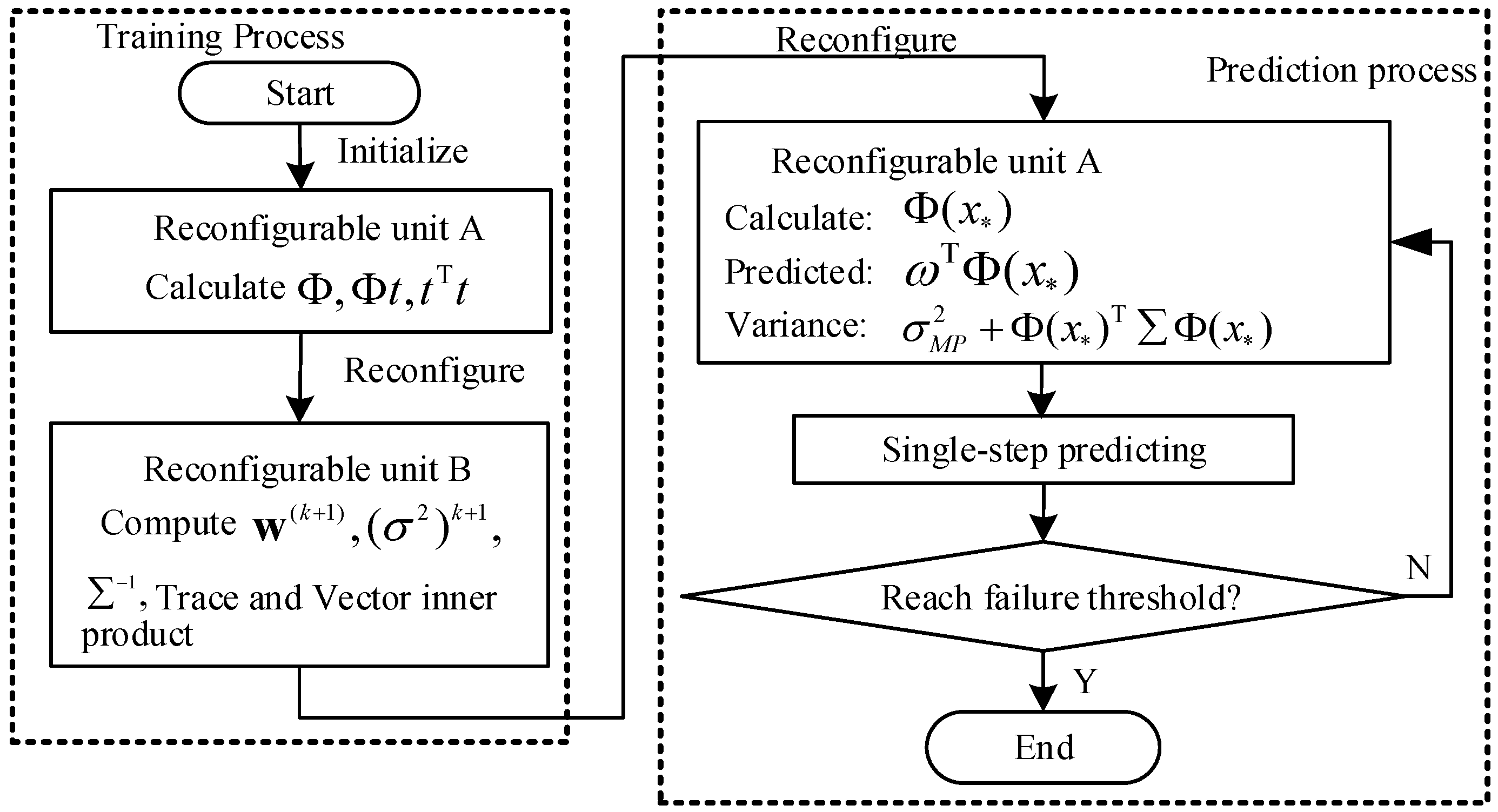
Figure 2 shows the flowchart of the proposed dynamic reconfigurable RVM based on the RC platform. The RVM in this platform has a training phase and a prediction phase, which compose a typical online retraining process. The FPGA is initially configured as unit A in the training phase and store the intermediate results in unit A. Then, the FPGA is reconfigured as unit B and store the calculated results in unit B. In the prediction phase, the unit A is reconfigured to predict the fault growth and estimate the RUL. From this figure, it is obvious that the training phase involves one reconfiguration from unit A to unit B and the prediction phase involves one reconfiguration from unit B to unit A. The online re-training process of RVM needs two dynamic reconfigurations for each cycle of computation.

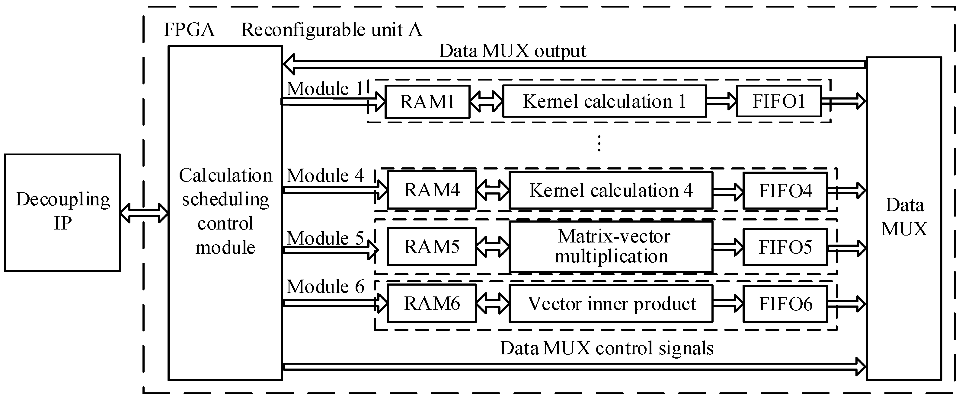
Figure 3 shows a general framework of dynamic RC system on Virtex-5 FPGA [24]. The dynamic RC system consists of FPGA, off-chip memory, and configuration memory.

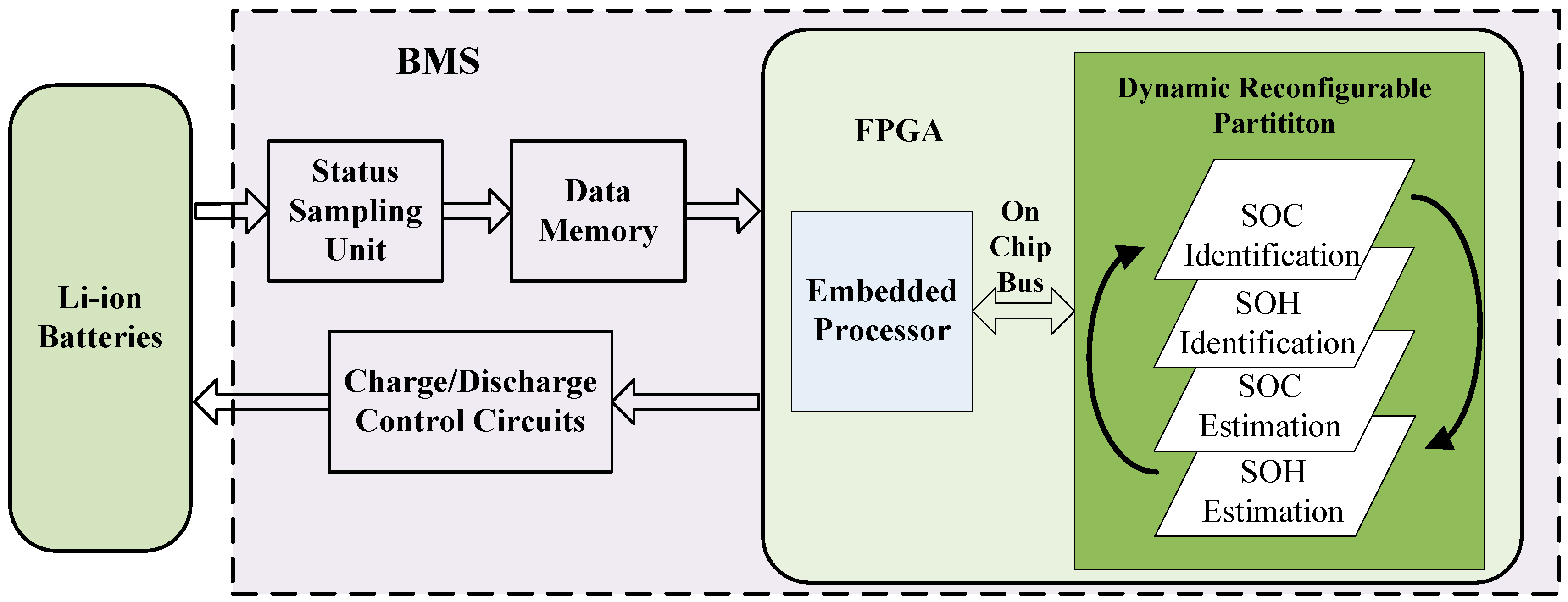
FPGA is the core functional unit that comprises a static logic partition and dynamic reconfigurable partition. The static logic partition includes embedded processors, on-chip bus, and peripheral modules connected to the bus. Dynamic reconfigurable partition executes reconfiguration units A and B in time multiplexing mode for RVM training and prediction. The embedded processors access the dynamic reconfigurable partition through the on-chip bus to control the computing process.

Off-chip memory stores the input data and intermediate results for RUL prediction. Data exchange between the dynamic reconfigurable partition and off-chip memory is implemented in direct memory access (DMA) manner to improve data transmission efficiency. Decoupling IPs are used to avoid disturbing the functions of static logic partition during dynamic reconfiguration. The configuration memory is used to store FPGA configuration files.

4.4.2. Architecture of Dynamic Reconfigurable Partition

The internal structures of the reconfiguration units A and B are designed as shown in Figure 4 and Figure 5. The internal architecture of the dynamic reconfigurable partition is a key factor to ensure the efficient task execution. The modular design is utilized to divide reconfiguration units A and B into several computing modules. To balance the resources of reconfigurable units and leverage the parallel computing features of FPGA, four processing elements (PE) of kernel functions are instantiated to synchronously calculate the Gaussian kernel.

In Figure 4, the reconfiguration unit A includes six main calculation modules, in which modules 1–4 are parallel PEs of kernel function, module 5 is a matrix-vector multiplication module, and module 6 is vector inner product module. The reconfiguration unit B shown in Figure 5 consists of five modules, in which module 1 is for matrix multiplication, module 2 is for improved Cholesky decomposition, module 3 is for matrix inversion, module 4 is for matrix-vector multiplication, and module 5 is for vector inner product.

The interface between the reconfiguration partition and the static logic partition must be consistent. It includes on-chip bus interface and the control interface for data and commands transmission. Calculation control module ensures that the computing tasks are executed in sequence with the scheduled timing. First-in-first-out (FIFO) is for buffering the calculation results and RAM is for buffering the input data and intermediate variables. The inputs and outputs of the FIFO and RAM are controlled by the Calculation control module related to specific computing task.

4.4.3. Design of Key Modules

The kernel function computing involves calculation of 2-norm and exponential functions. The 2-norm calculation has low computation efficiency since it cannot be executed with pipeline computing while the exponential function is a transcendental function which cannot be directly implemented by multiplier and adder. To achieve high efficiency, a multi-level pipeline calculation method of piecewise linear approximation is proposed. In addition, an improved Cholesky decomposition method is proposed to accommodate the large amount of computations in matrix inversion with lower-upper (LU) decomposition and the instability caused by the round-off error from the Cholesky decomposition.

• Multi-level pipelined calculation method of piecewise linear approximation for the kernel function

For Gaussian kernel function $K(x,x_i)=\exp (-{\Vert x-x_i\Vert }_2^2/{\gamma }^2)$ where $\gamma$ is the hyper-parameter determined before training, the kernel matrix $\Phi$ is a symmetric positive definite matrix whose diagonal elements are all 1. Therefore, only the lower triangular elements, as shown below, need to be calculated:

$${\Phi }_{\text{lower}}=\left[\begin{array}{ccccc}1& & & & \\ k(x_2,x_1)& 1& & & \\ k(x_3,x_1)& k(x_3,x_2)& \ddots & & \\ ⋮& ⋮& ⋮& 1& \\ k(x_n,x_1)& k(x_n,x_2)& \cdots & k(x_n,x_{n-1})& 1\end{array}\right]$$

(20)

(a)

2-Norm Calculation

Assuming that the dimension of training samples is $l$, the 2-norm for vector $x_i$ and $x_j$ is:

$${\Vert x_i-x_j\Vert }_2^2={(x_{i1}-x_{j1})}^2+{(x_{i2}-x_{j2})}^2+\cdots +{(x_{il}-x_{jl})}^2$$

(21)

A multi-level pipelined method is introduced to calculate the 2-norm. Take the first column in Equation (20) as an example, the computing elements are shown in

Table 1. Computing components for the 2-norm computation.

2-Norm	1st Step	2nd Step	$\cdots$	lth Step
${\Vert x_2-x_1\Vert }_2^2$	$a_1={(x_{21}-x_{11})}^2$	$a_n={(x_{22}-x_{12})}^2$	$\cdots$	$a_{(l-1)*(n-1)+1}={(x_{2l}-x_{1l})}^2$
${\Vert x_3-x_1\Vert }_2^2$	$a_2={(x_{31}-x_{11})}^2$	$a_{n+1}={(x_{32}-x_{12})}^2$	$\cdots$	$a_{(l-1)*(n-1)+2}={(x_{3l}-x_{1l})}^2$
$⋮$	$⋮$	$⋮$	$⋮$	$⋮$
${\Vert x_n-x_1\Vert }_2^2$	$a_{n-1}={(x_{n1}-x_{11})}^2$	$a_{n+n-2}={(x_{n2}-x_{12})}^2$	$\cdots$	$a_{(l-1)*(n-1)+\mathrm{n}+1}=={(x_{nl}-x_{1l})}^2$

.

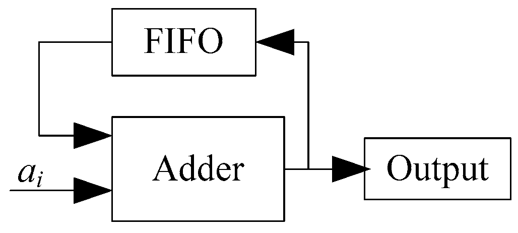
The 2-norm computing process is executed by rows. That is, ${\Vert x_2-x_1\Vert }_2^2$ is first and then ${\Vert x_3-x_1\Vert }^2$, and so forth. In this process, a fully pipelined accumulator is designed with an fully pipelined adder and a FIFO as shown in Figure 6.

Figure 7 shows the computing flowchart of the fully pipelined accumulator. In the first stage, data a₁, a₂, ..., a_n−1 and “0“ are input to the adder, and the outputs of the adder are stored in the FIFO. In the 2^nd stage, data a_n, a_n+1, ..., a_2(n−1) and FIFO buffered data from the 1^st stage are then input to the adder. The outputs of the adder are again stored in the FIFO. This process is repeated at the l^th pipeline cycle. Similarly, the 2-norm calculations in other columns can be implemented.

(b)

Exponential Function Calculation

Since exponential function cannot be implemented directly by adders and multipliers in FPGA, a piecewise linear approximation method, which combines linear polynomial function and LUT, is employed as an approximation [25]. In this method, the linear polynomial parameters are stored in the LUT while the calculation of linear polynomial is implemented by an adder and a multiplier in FPGA.

The principle of piecewise linear approximation is as follows: for a nonlinear function $f(x)$ defined in $x\in [L,U]$, the interval is evenly divided into m subintervals [L_i, U_i] and $m=(U-L)/(U_i-L_i)$. For $x\in [L_i,U_i]$, $f(x)$ is approximated as $f(x)=k_{i}x+b_i$, where $k_i$ and $b_i$ are linear polynomial parameters stored in the LUT. Note that m introduces trade-off between accuracy and hardware occupation and should be selected properly.

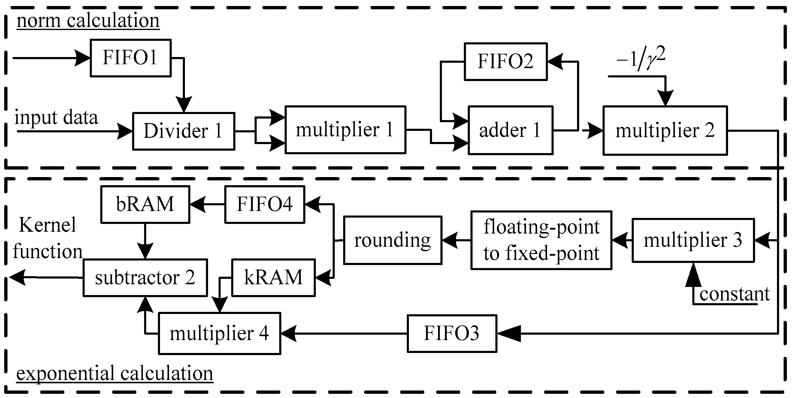
Figure 8 shows the data path of Gaussian kernel function calculation. In this figure, the upper part is for 2-norm calculation while the lower part is for exponential function calculation. In the lower part, bRAM and kRAM store parameters k and b for piecewise linear approximation, respectively.

The corresponding values of k and b can be obtained by accessing the addresses for these two RAMs. Then the kernel function can be calculated with subtractor 2 and multiplier 4. To get the right addresses of bRAM and kRAM, the output of the 2-norm calculation is mapped to the RAM address by multiplication, “floating-point to fixed-point” and rounding units.

Since the computing delay of multiplier 4 is one clock cycle larger than subtractor 2, FIFO4 is used to synchronize them by introducing a clock delay to access the bRAM. FIFO3 is used to store the output of 2-norm calculation and its depth should be larger than the delay of multiplier 4, which is 8 clock cycles in this design. The multiplier and adder are implemented with Xilinx floating-point arithmetic IP core, and the data are in single-precision floating point format.

• Improved Cholesky decomposition for matrix inversion based on multiply subtraction

To make computations affordable and deal with the instability caused by rounding error in of matrix inversion computing process, an improved Cholesky decomposition [26] is introduced for the inversion of symmetric positive definite Gaussian kernel matrix $\sum$. The improved Cholesky decomposition method decomposes matrix $\sum$ as follows:

$$\sum =\mathit{L}\mathit{D}{\mathit{L}}^{\mathrm{T}}$$

(22)

where L is a lower triangular matrix whose diagonal elements are all 1, D is a diagonal matrix (its diagonal elements are not 0). Matrices L and D can be obtained as:

$$\{\begin{array}{l}{d}_r=\left(h_{rr}-{\displaystyle \sum _{k=1}^{r-1}{l}_{rk}^2{d}_k}\right),\\ l_{ir}=\left(h_{ir}-{\displaystyle \sum _{k=1}^{r-1}{l}_{ik}{d}_k{l}_{rk}}\right)/d_r.\end{array}$$

(23)

where $r=1,\cdots ,n,i=r+1,\cdots ,n$ and $h$ is the element of $\sum$.

Assuming $P={\mathit{L}}^{-1}$, we have ${\sum }^{-1}=P^{\mathrm{T}}{\mathit{D}}^{-1}P$, where P is a lower triangular matrix with elements of:

$$\{\begin{array}{l}{p}_{ii}=1/l_{ii}=1\\ p_{ij}=-p_{ii}{\displaystyle \sum _{k=j}^{i-1}{l}_{ik}{p}_{kj}=-}{\displaystyle \sum _{k=j}^{i-1}{l}_{ik}{p}_{kj}}\end{array}$$

(24)

where $i=1,2,\cdots n,j=1,2,\cdots i-1$.

The implementation of the improved Cholesky decomposition and matrix inversion is shown in Figure 8. The elements in diagonal matrix D⁻¹ is the reciprocal of corresponding elements in matrix D and this only requires division. The computation of matrix P, i.e., the inverse matrix of L, is given by Equation (24), in which $p_{ii}=1$ and $p_{ij}$ is the negative value of the result from a multiply accumulator:

In Figure 9, the calculation of D⁻¹ is achieved with divider 1 and the results are stored into FIFO1. Multiplier 1, subtractor 1 and FIFO2 are used to calculate the p_ij, in which FIFO2 buffers the results from the subtractor 1, which is initialized as 0. The memory depth of FIFO1 and FIFO2 is n. With D⁻¹ and P, ${\sum }^{-1}$ can be calculated by ${\sum }^{-1}=P^{\mathrm{T}}{\mathit{D}}^{-1}P$.

5. Discussion System Performance Testing and Evaluation

5.1. Hardware Platform

The run-time dynamic RC system must be implemented on reconfigurable devices for onboard and distributed applications. To verify the proposed run-time dynamic RC system for RVM-based lithium-ion batteries RUL estimation, the Xilinx ML510 development board is used. In the experiments, accuracy, computational efficiency, and hardware resource consumption for the reconfigurable RVM based RUL prediction system are analyzed and discussed.

The main specifications for ML510 development board are as follows:

• FPGA: Virtex XC5VFX130T;
• DDR2 SDRAM: 512 MB, 72-bit and 2 chips;
• CompactFlash (CF): 512 MB.

A run-time RC RVM system is constructed as shown in Figure 10, in which the embedded processor PowerPC440 has a working frequency of 400 MHz, the on-chip PLB bus has a working frequency set to 100 MHz, the configuration port is the ICAP interface embedded in the XC5VFX130T, and the floating-point arithmetic computing is implemented with the single-precision floating-point IP core based on IEEE754 standard [27] provided by Xilinx ISE 13.2 (San Jose, CA, USA). For comparison purposes, a PC platform with a 2.53 GHz Core 2 Duo CPU, and 2 G DDR2 memory is used to execute the same algorithm.

5.2. Lithium-Ion Battery Data Set

Two lithium-ion battery data sets are used to verify the proposed framework. One is from the data repository of the NASA Ames Prognostics Center of Excellence (PCoE) and the other one is from the CALCE at the University of Maryland.

The first data set was sampled from a battery prognostics test bed at NASA comprising commercially available Li-ion 18650 rechargeable batteries [28]. The lithium-ion batteries were run through three different operational profiles (charge, discharge, and impedance) at room temperature. Charging was carried out in a constant current mode at 1.5 A until the battery voltage reached 4.2 V and then continued in a constant voltage mode until the charge current dropped to 20 mA. Discharge was carried out at a constant current level of 2 A until the battery voltage fell to 2.7 V, for battery B5. Repeated charge and discharge cycles resulted in accelerated aging of the batteries. The experiments were stopped when the batteries reached the end-of-life criterion, which was a 30% fade in rated capacity.

In the CALCE data set, the cycling of battery CS2-33 was implemented with the Arbin BT2000 battery testing system (made by Arbin Instruments, College Station, TX, USA) under room temperature. The 1.1 Ah rated capacity of batteries are adopted in the experiment with the discharging rate at 0.5 C [15,29].

5.3. Prediction Precision of RUL Estimation

In this Section, the battery data sets are used to verify the performance of the run-time dynamic RC system for RVM, and the results are compared with those from the PC platform. The quantitative prediction results for B5 and CS2-33 batteries are summarized in

Table 2. RUL prediction comparison between FPGA and Matlab.

Index	Platform	RULa	RULp (mean)	95% CI	AE	${\eta }_{AE}$
B5	FPGA	48	45	[34, 49]	3	4.2%
	PC		49	[41, 54]	1
CS2-33	FPGA	240	231	[222, 248]	9	2.5%
	PC		225	[208, 238]	15

. The prediction starting points are selected at the 80^th cycle for B5 battery and 278^th cycle for the CS2-33 battery, respectively. The failure thresholds for the two batteries are set to 1.38 Ah (about 30% fade) and 0.88 Ah (about 20% fade). In this table, the performances are compared by the predicted RUL (RULp) values (given by the mean of the predicted RUL distribution), the Absolute Error (AE) (given by the difference between the actual RUL (RULa) and RULp), the predicted precision ratio of two platforms (${\eta }_{AE}$) (given by the ratio of absolute difference of AE to RULa), and 95% confidence intervals (CI).

From Table 2, it is clear that the results from the two platforms have comparable accuracy. The prediction precisions on the RC platform are 4.2% and 2.5% different from that on the PC platform for the two batteries. This is because the RC platform uses single-precision computing while the PC platform adopts double-precision computing, but these minor differences are acceptable for industrial applications. Note that the predicted confidence intervals from the two platforms are very close to each other. The experimental results show that RUL prediction with dynamic reconfigurable RVM on the FPGA platform is comparable to the prediction on the PC platform.

5.4. Analysis of Computing Efficiency

To quantify the improvement on computational efficiency of the proposed method, the computing processes of lithium-ion battery RUL prediction in Section 4.3 is analyzed. The speed-up ratio is defined as:

$${\eta }_t=\frac{T_{PC-RVM}}{T_{RC-RVM}}$$

(25)

where T_RC-RVM is the executing time with RC platform and T_PC-RVM is with PC platform. It is clear that ${\eta }_t$ > 1 indicates that the RC-based RVM algorithm has higher computational efficiency than the PC platform. The larger the ${\eta }_t$, the higher the increase of the efficiency.

The comparison is summarized in

Table 3. Efficiency comparison between FPGA and PC.

Index	Platform	TT (ms)	PT (ms)	N.R	O.R (ms)	OT (ms)
B5	FPGA	96.70	7.32	2	16.99	138.00
	PC	614.02	11.81	0	0.00	625.83
	Speed-up ${\eta }_t$	6.35	1.61	0	0.00	4.54
CS2-33	FPGA	524.25	69.27	2	16.99	627.50
	PC	6287.30	185.62	0	0.00	6472.92
	Speed-up ${\eta }_t$	11.99	2.68	0	0.00	10.31

TT; Training time; PT: Predicting time; N.R: No. of reconfigurations; O.R: Overhead per reconfiguration; OT: Overall time.

, which shows that RC based RVM in FPGA has higher efficiency than the PC platform in terms of training, prediction, and overall. For prediction part with low computational complexity, the speed-up ratios for the battery B5 (small prediction steps) and the battery CS2-33 (relatively large prediction steps) are 1.61 and 2.68, respectively. For training part with high computational complexity, the speed-up ratios for the battery B5 and the battery CS2-33 are 6.35 and 11.99, respectively. As for the overall efficiency, the speed-up ratios for the two batteries are 4.54 and 10.31, respectively. This demonstrates that the proposed RC-based RVM in FPGA platform has great potentials in improvement of computational efficiency, especially for complex tasks.

The FPGA power is about 4.94 W by Xilinx Power Estimator and the power of the CPU is about 25 W from its datasheet, so the FPGA consumes 0.68 J and 3.10 J energy, which are 22.97× and 52.17× less than CPU, for B5 and CS2-33 RUL prediction, respectively. This further demonstrates that FPGA is more suitable for embedded and power aware application.

5.5. Analysis of Hardware Resource Consumptions

To verify the adaptability and applicability of the proposed method, the hardware resources, including the utilization of static and dynamic partition throughout the FPGA, are analyzed. The analysis also shows the improvement of resource utilization of the dynamic RC against the static reconfiguration.

The required hardware resources of RC RVM approach and the available FPGA resources are shown in

Table 4. FPGA resource utility.

Categories	PowerPC	LUTs	BRAM	DSP48E
Static partition	1	4826	48	0
Dynamic partition	0	14,144	40	120
Total utilized resources	1	18,970	88	120
Total FPGA resources	2	81,920	298	320
Ratio of utilization	50.00%	23.16%	29.53%	37.50%

. The utilization ratio of DSP48E and BRAM is larger than that of LUTS (the logic resources) in our proposed method. This suits to the characteristics of the computing with FPGA IP core in which more DSP48E and BRAM resources are consumed. Note that more than 50.00% of the BRAM and DSP48E resources in FPGA are reserved, which demonstrates that the proposed method has great potentials to support more complex computation tasks with limited computing resources. And in another aspect, a smaller FPGA device, such as XC5VFX70T, can be used to accommodate the whole design. This better fits the requirements of the compact embedded BMS systems.

The improvement of the resources utilization by the dynamic RC algorithm can be further illustrated by comparing the resources occupation of the dynamic RC and static reconfiguration. The resource consumptions of dynamic area are obtained by Xilinx’s Plan Ahead design tool and the results are compared in

Table 5. The increase of hardware utility.

Items		LUTs	BRAM	DSP48E
Static	Reconfigurable unit A	9440	21	90
	Reconfigurable unit B	14,112	34	92
	Sum of two units	23,552	55	182
Dynamic	Dynamic partition	14,144	40	120
Resources saving		9408	15	62
Resources saving percentage		39.95%	27.27%	34.07%

. In Table 5, the resources consumption in the static reconfigurable algorithm is the sum of the reconfigurable units A and B, without considering the increased connectivity resources consumption. For dynamic RC, the resources consumption is those in the dynamic partition. Table 5 shows the dynamic resources saving includes 9408LUTs (39.95%), 15 BRAM (27.27%), and 62 DSP48E (34.07%). This result demonstrates that the proposed method has higher FPGA resource utilization and is more suitable for computing resources constrained applications.

The difference of DSP48E for two reconfigurable units in static reconfiguration is 2, which accounts for 2.17% of the maximum required DSP48E resources (92). This shows that the two reconfigurable units achieve the consumption balance of DSP48E. This further proves the effectiveness of the proposed method using multi-objective optimization for reconfigurable tasks partitioning in which the balance of DSP48E resources between different partitions is the main constraint.

The static reconfigurable implementation can be realized with logics combining reconfigurable unit A and reconfigurable unit B in DPR version. Then the training and forecasting process will consume the same time with DPR version, but it avoids two reconfiguration overheads (2 × 16.99 ms). From Table 3, the reconfiguration overheads are about 24.6% and 5.4% in the whole consumed time of the B5 and CS2-33 batteries’ prognosis respectively. By avoiding these overheads, the static reconfigurable implementation can get 1.33× and 1.06× speedup in B5 and CS2-33 batteries respectively compared to the corresponding dynamic reconfigurable implementation. Thus static reconfigurable implementation can get the computational performance a little bit improved, but at the cost of more hardware consumption as shown in Table 5 (39.95% more LUTs, 27.27% more BRAM, 34.07% more DSP48E). Regarding our motivation to get a more compact BMS, we think dynamic reconfigurable system is a better choice.

6. Conclusions

In this work, a novel run-time dynamic RC-based RVM prognostic algorithm and its implementation on a reconfigurable FPGA platform are developed for RUL estimation. The experiment results demonstrate that the embedded computing platform can significantly improve the computing efficiency and flexibility. The contributions of the research work include a balance of resources utilization and computing efficiency is achieved by multi-objective optimization method to implement computing tasks partitioning; the multi-level pipelined computing and parallel computing are developed for kernel function calculation to further improve the computational efficiency; the improved Cholesky decomposition for matrix inversion is introduced to reduce the computing resource consumption and decreases the computational delay; and thorough analysis and comparison of different embedded system configurations in terms of accuracy, resource utilization, and computation efficiency. Experimental results on two examples of lithium-ion battery RUL estimation show that the FPGA based run-time dynamic RC improves the hardware resources utilization and is more than four times faster than a PC-based approach without sacrificing performance. This work provides a novel solution for the implementation of prognostic prediction based on machine learning algorithm in embedded computing systems. In future, more algorithms, such as SOC estimation, prognosis in operation condition varying applications, etc., will be implemented in the proposed system.